Key Factors of the Initiation and Development of Polygonal Wear in the Wheels of a High-Speed Train

1
State Key Laboratory of Traction Power, Southwest Jiaotong University, Chengdu 610031, China
2
Mechanical Engineering College, Southwest Jiaotong University, Chengdu 610031, China
*
Author to whom correspondence should be addressed.
Appl. Sci. 2020, 10(17), 5880; https://doi.org/10.3390/app10175880
Submission received: 28 July 2020
/
Revised: 17 August 2020
/
Accepted: 20 August 2020
/
Published: 25 August 2020
(This article belongs to the Special Issue Tribology in Machine Components)
Abstract
:The polygonal wear of train wheels occurs commonly in rail transport and increases the wheel–rail interaction force dramatically and has a bad effect on the safety and comfort of the train. The mechanism of polygonal wear needs to be studied. The characteristics of test data measured from 47,000 sets of polygonal wheels of high-speed trains were analysed statistically. The analysis shows that, in the entire use life cycle of the wheels, the order (wavelength) and development speed of polygonal wear are different; they correspond to different wheel diameters because of wear and re-profiling. A prediction model, which considered the flexibility of the wheelset for the polygonal wear of the wheels of high-speed trains, was developed to explain this phenomenon. This theoretical model analyses the initiation, development, and characteristics of polygonal wear. The analysis includes the effect of the high-frequency flexible deformation of the wheelset, train operation speed, and wheel diameter variation. This study suggests that, if the wheel perimeter is nearly an integral multiple of the wavelength of severe periodic wear along the wheel circumference, the polygonal wear on the wheel can develop quickly. Furthermore, the wavelength of the periodic wear of the wheel relies on the operation speed of the train and wheelset resonant frequency. Therefore, the initiation and development of polygonal wear on wheels depends on the operation speed, wheel diameter, and the resonant frequencies of the wheelset. This conclusion can be applied to research concerning measures associated with the suppression of polygonal wear development.
1. Introduction
Polygonal wear is uneven wear along the circumference of train wheels and its wavelength varies from a dozen centimetres to the entire circumference of the wheel [1,2]. Polygonal wear with only one wavelength around the wheel circumference is called first-order polygonal wear (i.e., eccentric wear); that with two equal wavelengths is called second-order polygonal wear (i.e., elliptical wear); that with three equal wavelengths is called third-order polygonal wear, and so on. First-, second-, and third-order polygonal wear are considered low-order polygonal wear. In recent years, polygonal wear beyond the eighth order—defined as a high-order polygonal wear in the present research have often been detected on the wheels of high-speed trains, metro trains, and electric locomotives in China [2]. Polygonal wear increases wheel–rail interaction and has a considerable effect on the use life of the components of railway vehicles and tracks. Furthermore, it threatens operation safety [3]. Therefore, this problem has gradually become a matter of urgent public concern in the railway transportation industry in China, and globally, and thus, it has attracted the attention of many scholars over the last few years. Kaper identified polygonal wear phenomena on train wheels when he conducted research on the noise of intercity trains and studied the relationship between polygonal wear and noise in the frequency domain [4]. Nielsen and Jin reviewed the literature on wheel polygonal wear in 2000 and 2018, respectively, and in their review, they summarised numerical simulation models of polygonal wear and explanations on its initiation mechanism and development [2,3].
Morys developed a dynamics model of an ICE-1 high-speed Garman train to investigate the polygonal wear mechanism. In the model, the wheelset mass modelling included five parts (two wheels and three brake discs), and they were all regarded as rigid bodies [5,6,7]. Three-dimensional rotational spring-damper units were used as connections to characterize the bending and torsional properties of the wheelset. The results showed that the bending resonant modes of the wheelset were excited by the fluctuating vertical force of the wheel–rail, and this led to a scenario where the lateral creep force of the wheel–rail varied periodically and the polygonal wear occurred on the rolling circle of the wheel.
Based on the Morys’s simulation model, Meinke considered beam elements as connections instead of three-dimensional rotational spring dampers [8]. Then, the effect of rotational inertia, gravity, and the gyroscopic moment of the wheelset on the initiation of polygonal wear was considered. In addition, imbalance calculations and long-term wear simulation were performed.
Meywerk established a coupling dynamics model that included an elastic wheelset and two elastic rails to study the formation of polygonal wear [9]. The results showed that flexible deformations of the wheelset and rails, caused by their interaction, resulted in the initiation and development of polygonal wear. The first and second bending modes of the wheelset played an important role in initiating polygonal wear.
This literature focused on the characteristics and mechanisms of low-order polygonal wear. Chen proposed a finite element model of a wheelset’s rolling contact with two rails using commercial finite element software to conduct research to identify the root cause of polygonal wear [10]. Chen suggests that the self-excited vibration of the wheel–rail system leads to polygonal wear at a frequency of 150 Hz. A suitable sleeper support stiffness or wheel–rail friction coefficient can be controlled to limit the development of polygonal wear.
Tao et al. conducted extensive measurements of polygonal wear on electric locomotive wheels with radii of 1050–1200 mm at the average operation speed of 80 km/h [11,12]. The measurement results showed that the dominant orders of the polygonal wear of locomotive wheels were 18th, 19th, and 24th, and depended on wheel diameter. The initiation mechanism of the polygonal wear of the locomotive wheels is not captured in this paper.
Jin et al. studied the mechanism of the ninth-order polygonal wear in wheels of metro trains with a linear induction motor using a detailed site test and observation [13]. They found that the resonant frequency of the first wheelset bending matched the exciting frequency of the ninth-order polygonal wear. When the first wheelset bending mode was excited, the period of lateral creepage and force between wheel and rail occurred. Furthermore, the ninth-order polygonal wear gradually appeared.
Wu et al. studied the mechanism of polygonal wear of high-speed train wheels through extensive field tests [14]. The operation speed of the tested train was 250 km/h, and the diameter of the wheels was 860 mm. The results showed that the mechanism of wheel polygonal wear of high-speed trains could be attributed to the excited resonance of the train–track coupling system in operation and changing the operating speed could suppress the development of polygonal wear effectively.
In [13,14], the authors conducted many experiments to investigate the mechanism of high-order polygonal wear, but both studies lacked in-depth theoretical research and numerical simulation.
Wu et al. studied the root cause of high-order polygonal wear [15]. Their study concluded that there was a ~650 Hz bending mode of the rail segment between the front and rear wheelsets of the same bogie. This bending mode was identified as the primary contributor to polygonal wear. However, in the literature [15], the exciting frequency of the polygonal wear is 550–600 Hz, which does not match the bending mode frequency very well. The conclusions of this paper lack experimental verification.
Cai et al. presented a detailed investigation into the mechanism of metro wheel polygonal wear using on-site experiment numerical simulations [16]. The measurement results showed that more than 70% of the metro wheels had sixth- to eighth-order polygonal wear. In this paper, P2 resonance was suggested as the main contributor to polygonal wear, and the flexibility of the wheelset was also found to influence the formation of polygonal wear. However, this is not enough to explain the higher order polygonal wear, which occurred in high-speed conditions.
The literature discussed above provides a certain understanding of wheel polygonal wear problems. However, thus far, consistent understanding on the mechanism of polygonal wear is lacking. To understand the mechanisms of the initiation and development of high-order polygonal wear of railway wheels clearly, this paper conducts a detailed investigation into the high-order polygonal wear of the high-speed trains in China via extensive experimental analysis and numerical simulation.
The remainder of this manuscript is organised as follows: Section 2 analyses the data measured from more than 1000 sets of polygonal wheels in the field and provides information on the important relationship between polygonal wear order and wheel diameter size. Section 3 presents a simulation model to predict the initiation and development of polygonal wear. In Section 4 and Section 5, the model is used to verify the key conditions of initiation and the development of high-order polygonal wear and to calculate the relationship between polygonal wear and high-speed development, train operation speed, and wheel diameter change.
2. Characteristics of Polygonal Wear of High-Speed Wheels
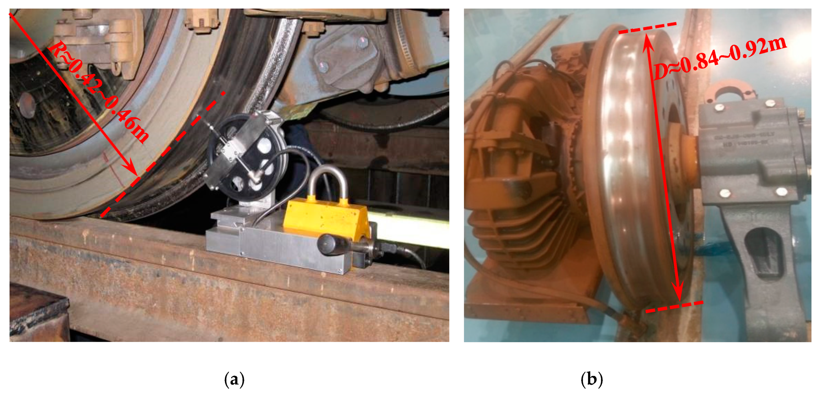
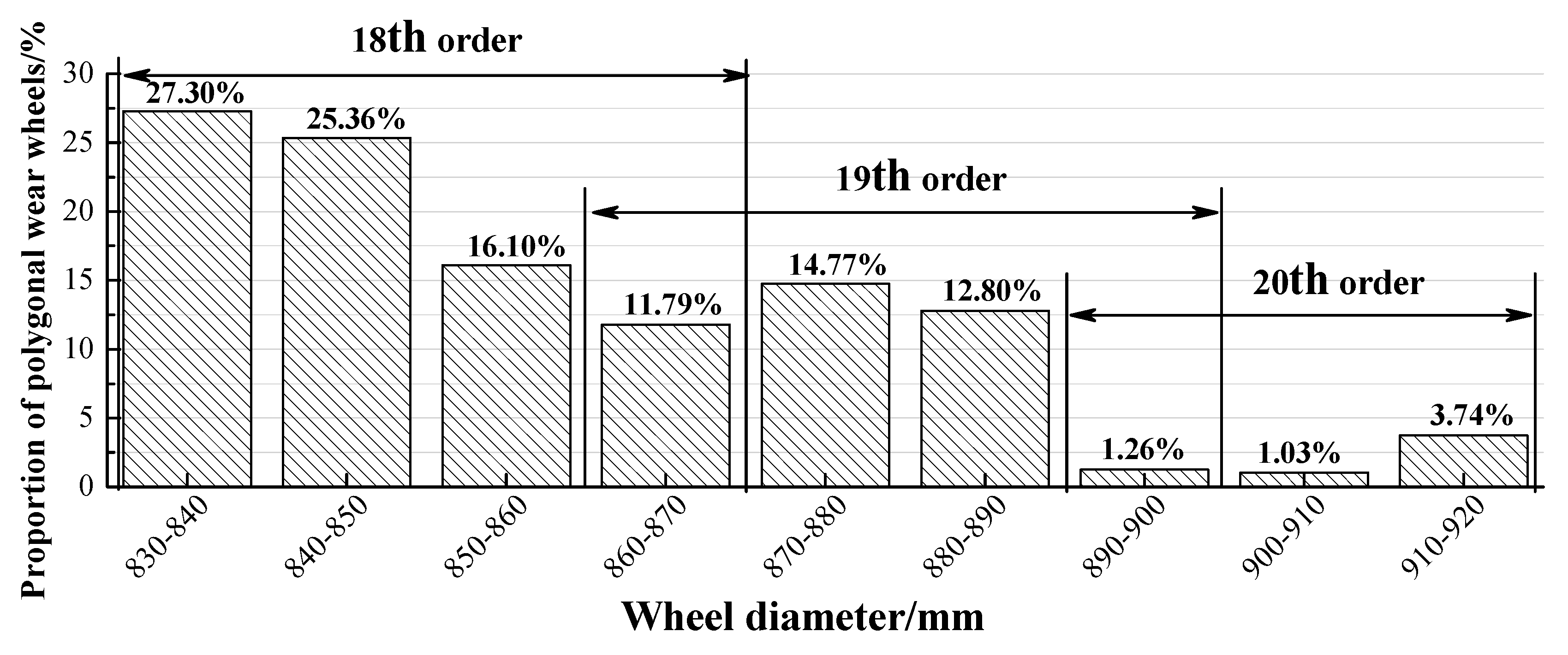
Polygonal wear occurs on the wheels of many high-speed trains. The census test of polygonal wear was conducted over a long time in this paper. The tested polygonal wheels comprised about 48,000 sets and the test mileage was >200,000 km after re-profiling. Figure 1a shows the Müller–BBM wheel roughness test instrument which was used for measuring polygonal wear, and Figure 1b shows a typical polygonal CL60 steel wheelset, which was provided by CSR Tangshan Rolling Stock Co., Ltd. During the test, the measured wheelsets were jacked up using hydraulic equipment so that the wheel could rotate around its axis line freely. The displacement sensor of the roughness test instrument contacts the wheel tread to measure the radial change in the wheel. Figure 2 shows the proportion of the polygonal wheel with a diameter change. The proportion of the polygonal wheel represents the quotient, which is the number of polygonal wheels divided by the number of all measured wheels with diameters of 830–840 mm, 840–850 mm, and 910–920 mm. A diameter of 920 mm is the nominal diameter for new high-speed wheels.
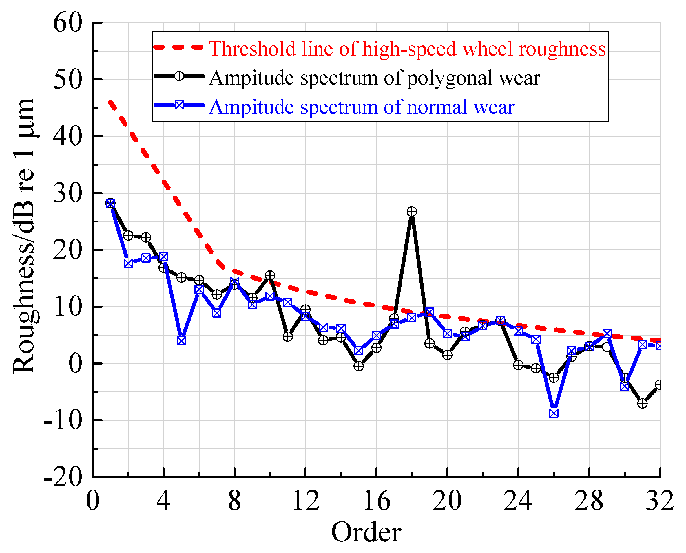
In the analysis, shown in Figure 2, the threshold of “high-speed” rail roughness (ISO-3095 Third edition 1 August 2013) was used as the threshold for high-speed wheels because there are no official partition criteria in China railways so far. Temporary (suggested) partition criteria for polygonal wear and non-polygonal wheels are designed by rolling stock companies and railway transport departments in China based on their requirements. The temporary partition criteria consider the rail roughness threshold line specified in ISO-3095 for the maintenance of high-speed wheels with severe polygonal wear. If the depths (peak to valley) of the polygonal wear of some dominant orders exceed the high-speed wheel roughness threshold line, the occurrence of the polygonal wear phenomenon is confirmed. As shown by the black line in Figure 3, the peak of 18th-order exceeds the roughness threshold line; thus, the wheel is regarded as a polygonal wheel. For the blue line in Figure 3, there is no peak exceeding the roughness threshold; thus, the wheel is regarded as a normal wheel. It is noted that ISO-3095 shows that the threshold line of rail roughness includes the wavelengths of 0.3 cm to 40 cm only. The polygonal wear of high-speed wheels covers the wavelengths of 12 cm to the whole wheel circumference. However, the wavelengths of the polygonal wear, which are much more concerned with the point view of controlling dynamic behaviour and noise, are in the range determined by the ISO-3095.
Through the statistical analysis of the test data, the characteristics of polygonal wear can be concluded as follows:
- Wheels with different diameters have different proportions of polygonal wheels and different dominant orders (main wavelength) of polygonal wear (Figure 2). Furthermore, it seems that the smaller the diameter, the higher the proportion of the polygonal wheels. This depends on the depth of the decarburised layer on the surface of the wheel.
- The proportion of polygonal wheels exhibits a non-monotonic variation as a function of the wheel diameter, including three local maxima around 830–840 mm, 870–880 mm, and 910–920 mm, corresponding to three periods of high-rate development.
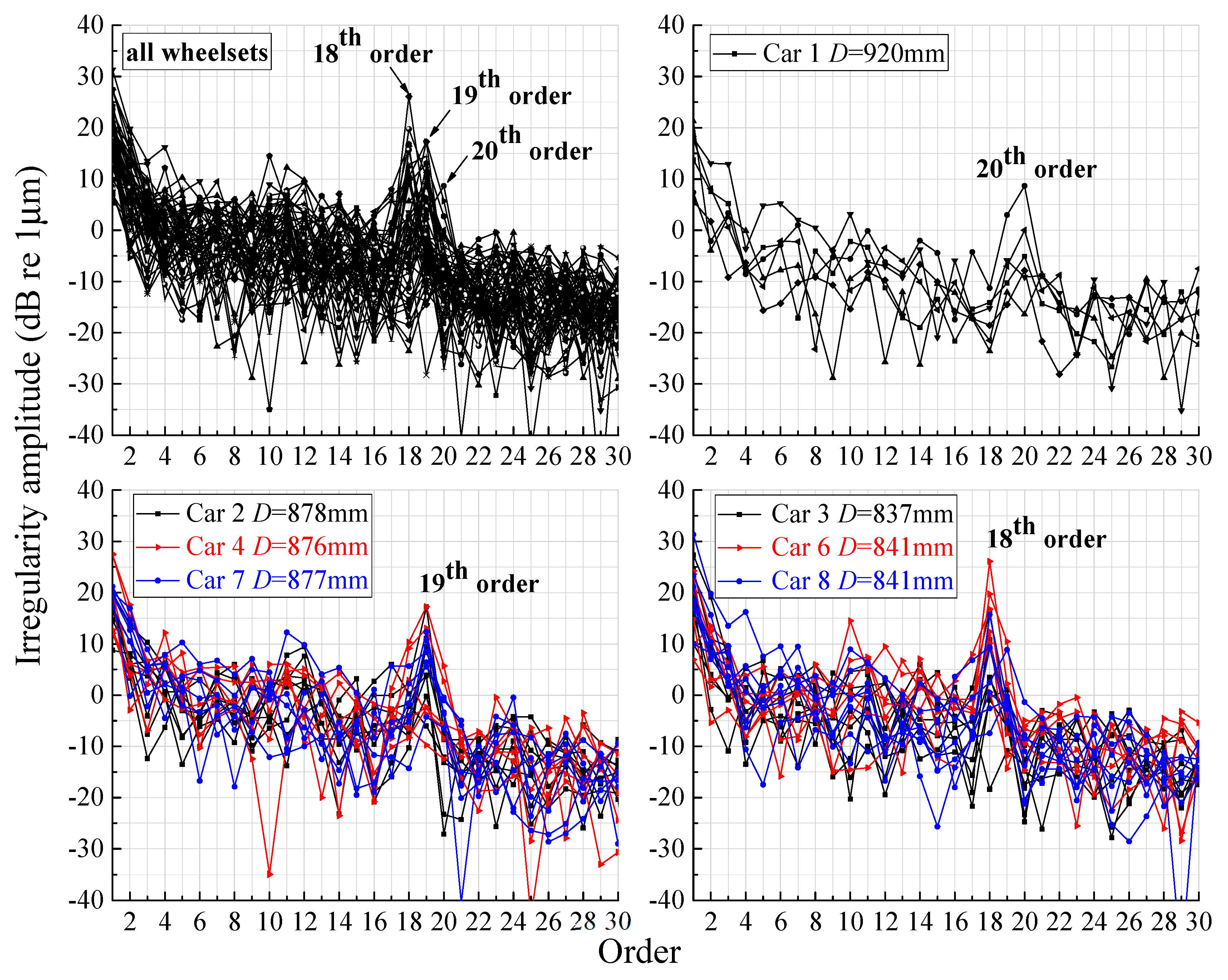
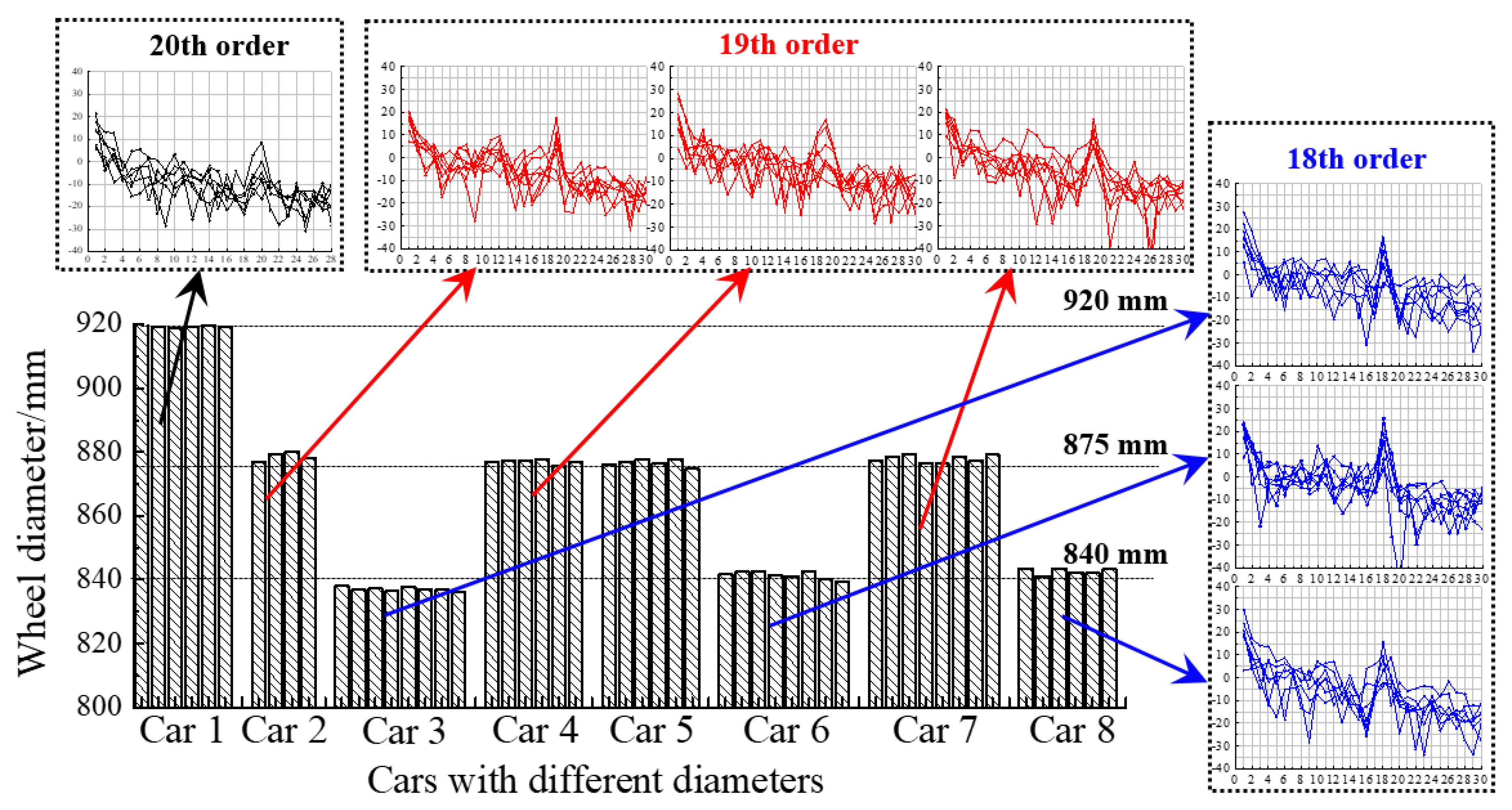
Figure 4 shows the roughness spectra of polygonal wear, measured from different cars for a typical high-speed train. The subgraphs show that different cars have different polygonal wear orders. The polygonal wear of the 20th order occurred on Car 1; 19th order occurred on Cars 2, 4, and 7; 18th order occurred on Cars 3, 6, and 8.
Figure 5 denotes the diameter change in the wheels corresponding to the polygonal wear of different orders that occurred on this typical train. The wheels of the tested train had different diameters, and this was not done intentionally. This high-speed train was used as a test train for long-term follow-up investigations into the dynamic behaviours and wear states of wheels/rails. The diameters of the wheels of the train were different because of the wear and re-profiling caused by an increase in operational mileage. The polygonal wear and fatigue states of the wheels determine their metal cutting quantity during re-profiling. Therefore, the cutting quantities of the wheels in re-profiling were different. Figure 5 shows that the wheels with diameters of ~920 mm generated a 20th-order polygonal wear; those with an 875 mm diameter produced 19th-order wear; those with 830–840 mm diameters formed 18th-order polygonal wear. This clearly indicates that a decrease in the diameter leads to a decrease in the polygonal wear order. Furthermore, the measured results of the wheels of car 5 do not indicate polygonal wear in Figure 4 and Figure 5 because the re-profiling of its wheels was conducted just before polygonal wear measurement.
The exciting frequency of the polygonal wear is calculated as:
where f denotes the exciting frequency of the polygonal wear, v denotes the operating speed of the vehicle, D denotes the diameter of the wheel, and n represents the polygonal wear order. Equation (1) indicates that wheels with different diameters have different polygonal wear orders at the same exciting frequency. For the present test case, f is ~570–580 Hz. This means that the wheels are excited in the frequency range of 570–580 Hz, and could produce the 18th to 20th order polygonal wear, corresponding to different wheel diameters. Therefore, it is necessary to clearly find where the 570–580 Hz vibrations are coming from (the vehicle or the track or their coupling resonance). That is the key to explaining the mechanism of initiation and development of high-order polygonal wear, and this will be further discussed later.
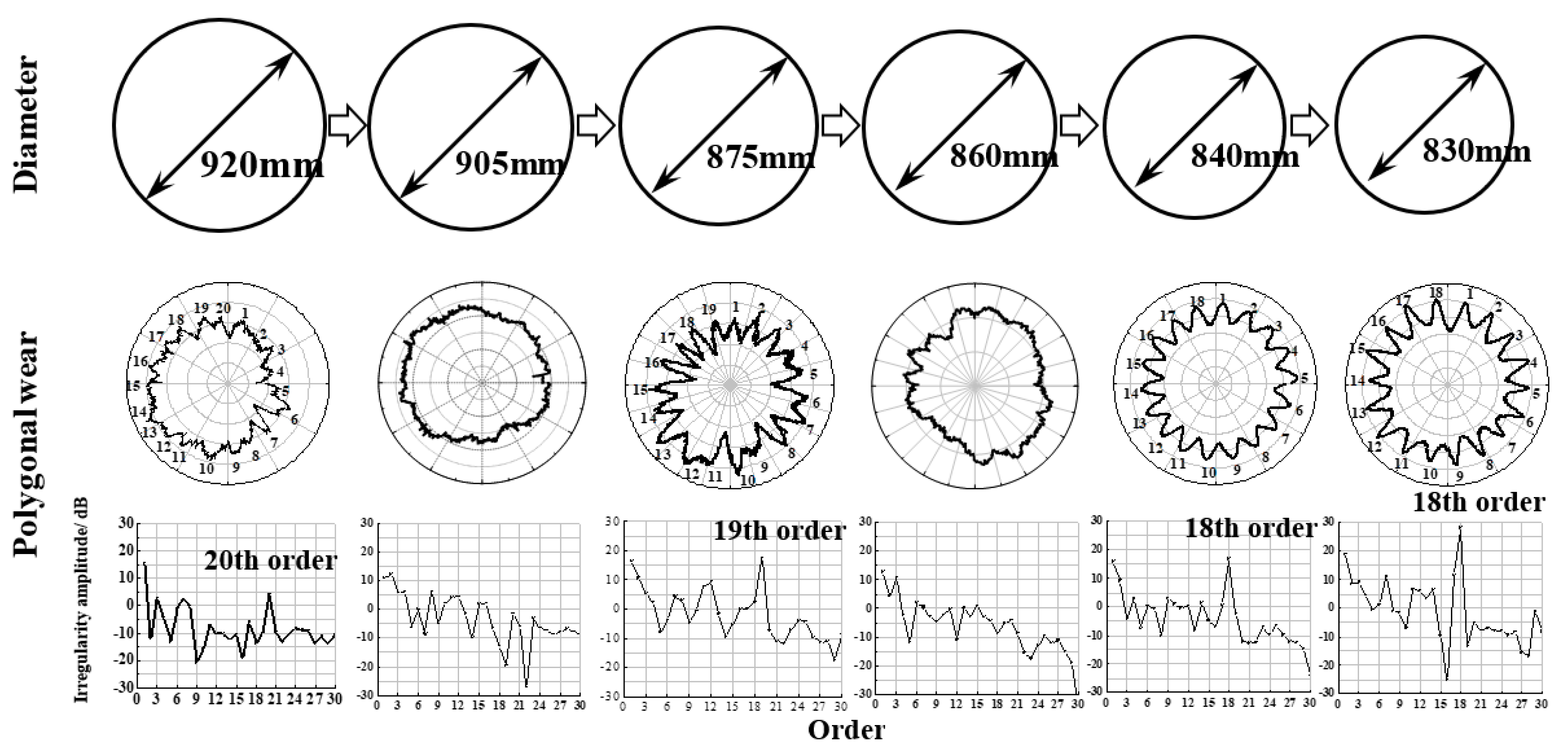
The test results of the same train are shown in Figure 6. The first row in Figure 6 indicates the wheel diameter reduction from 920 to 830 mm; the second row denotes the polygonal wear described in the polar coordinate system corresponding to different wheel diameters; the third row illustrates the order of the polygonal wear, which is also called the roughness spectra of the polygonal wear. In the test, the train operation speed was 300 km/h. The interval of wheel re-profiling was 200,000 km. Figure 6 shows the states of polygonal wear at six different wheel diameters—920, 905, 875, 860, 840, and 830 mm. The nominal diameter of new wheels is 920 mm, and 830 mm is the diameter close to the end of the wheel use life. During service, the wheel diameter changes from large to small because of wear and re-profiling. Indeed, at wheel diameters of ~920, 875, and 830–840 mm, a polygonal wear of the 20th, 19th, and 18th orders occur, respectively. According to Equation (1), the passing frequencies of the polygonal wear of three different orders or the resultant exciting frequencies between the wheel and rail are ~580 Hz at 300 km/h. Figure 6 further indicates that polygonal wear develops at a high rate at the three stages, at which the wheel diameters decreased in their whole use life, and they are, respectively, the initial stage of new wheel use, the wheel diameter near 875 mm, and the stage when the diameter is between 840 and 830 mm, in the present investigation case. Further, this phenomenon can be illustrated using Figure 5. For a wheel diameter around 905 and 860 mm, irregular wear with periodic character or equal-wavelength, or polygonal wear, is not serious.
From the statistical results of the tracking test in the field, the most prominent feature of polygonal wear is that there is nearly a one-to-one relationship between the wave number (or dominant order) of the polygonal wear and wheel diameter. For different wheel diameters, the wavelengths (or passing frequencies) of polygonal wear are considerably near at a constant operation speed, which suggests that the vehicle system in operation generates a vibration at nearly the same resonant frequency, thereby causing polygonal wear on the wheels. The resonance of the vehicle leads to polygonal wear. The smaller the diameter, the smaller the wave number.
3. Simulation Model
3.1. Rigid–Flexible Coupling Dynamical Model of Vehicle–Track
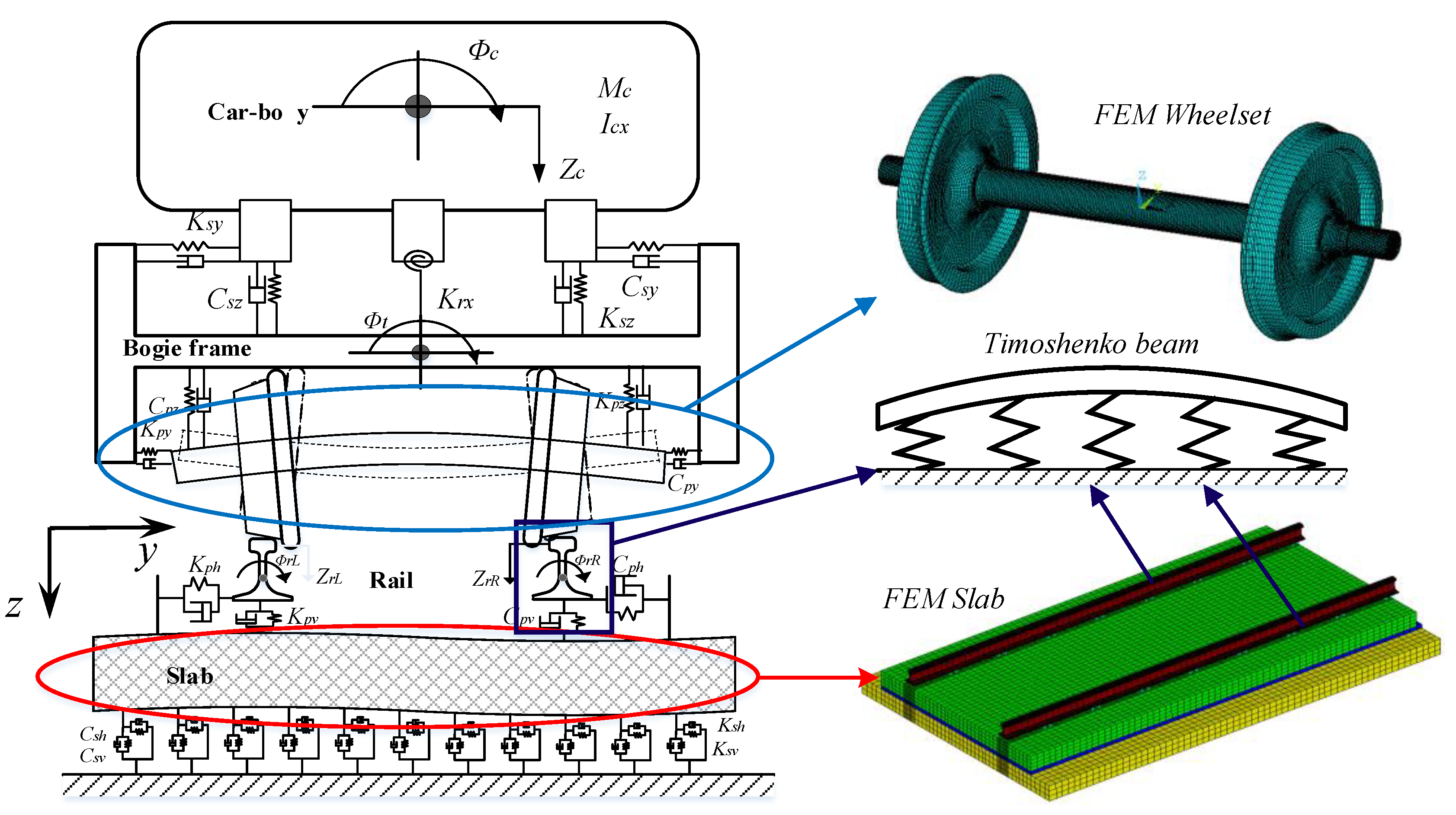
Figure 7 shows the rigid–flexible coupling dynamical model of vehicle/track [17,18,19,20,21,22,23]. The vehicle system model includes a car body, two bogies, and four wheelsets. The car body and frames of the two bogies are modelled as rigid bodies, and they each have five degree of freedoms. Wheelset structural flexibility is modelled using the finite element method and solved using the mode superposition method. The primary and secondary suspension systems of the vehicle are modelled with three-dimensional spring-damper elements. The track system is modelled as a monolithic track-bed system that includes rails, fasteners, slabs, and roadbed. The rails are modelled as Timoshenko beams with elastic discrete point support. Slab structural flexibility is considered using the finite element method and solved by using the mode superposition method [19]. The fastener is modelled using three-dimensional spring-damper elements. The roadbed support layer is modelled with equally distributed spring-damper elements. The parameters of the track and vehicle system are listed in Table 1.
According to the solid finite element theory, the differential equation of vibration of wheelset is written as
where the acceleration vector of the nodes on the ith wheelset at time t, is the velocity vector of the nodes on the ith wheelset at time t, is the mass matrix of the ith wheelset, is the stiffness matrix of the ith wheelset, and is the force vector of the nodes on the ith wheelset at time t, and it contains wheel–rail forces and primary suspension forces.
The modal superposition method is used to decouple
where is the vector of the kth order modal displacement on the ith wheelset and is the kth order modal coordinates on the ith wheelset at time t.
A dynamic explicit integral algorithm is used to solve this equation [17]. Finally, the displacement of the nodes in natural coordinates can be obtained.
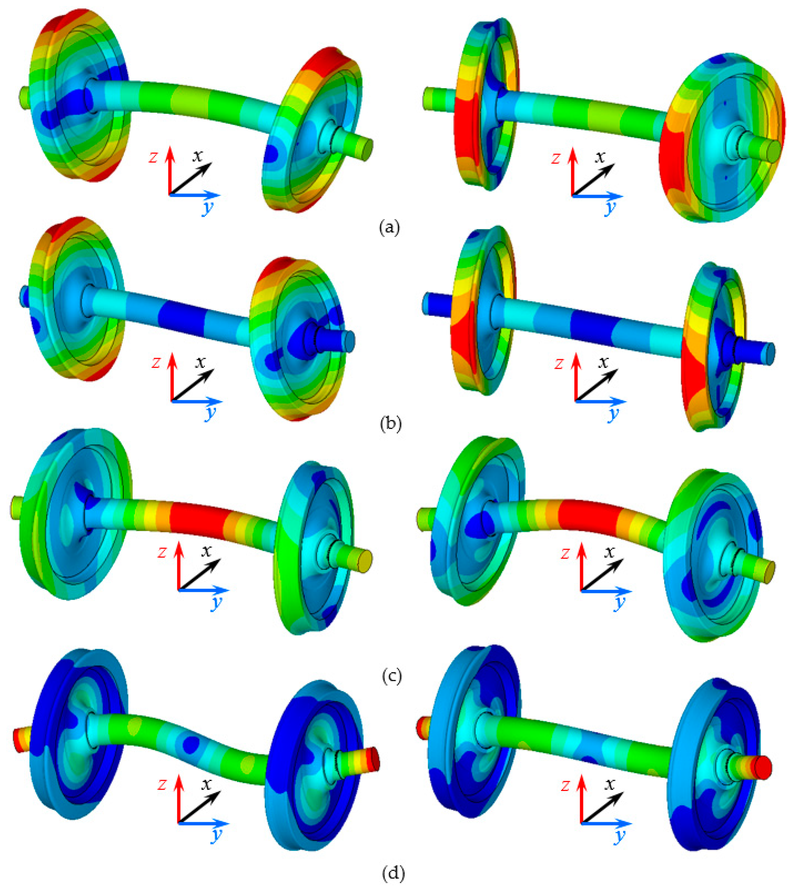
The finite element method was used to analyse the mode characteristics of the wheelset. The Hypermesh was used to mesh the geometric model of the wheelset, which was provided by the supplier of the wheelset. The element type was Solid45 and the element count was 255,360; the node count was 267,771. Then, the shape testing of all elements was conducted to ensure that a sufficiently fine mesh was used. The summary of the shape testing and the proofs of result independency to mesh size are placed in the Appendix A at the end of the manuscript (Table A1 and Table A2; Figure A1). The Block Lanczos method in ANSYS was used for modal analysis. Figure 8 shows the bending modes of the wheelset within a range of 800 Hz. The deformation of the wheelset includes mode deformation coupling in the two directions. In the vertical and longitudinal directions, there are same bending modes that have the same frequency and mode shape. Here, the mode at 576 Hz merits attention, because the frequency is very near to the exciting frequency of the polygonal wear, according to Equation (1).
3.2. Method for Online Searching Wheel–Rail Contact Points
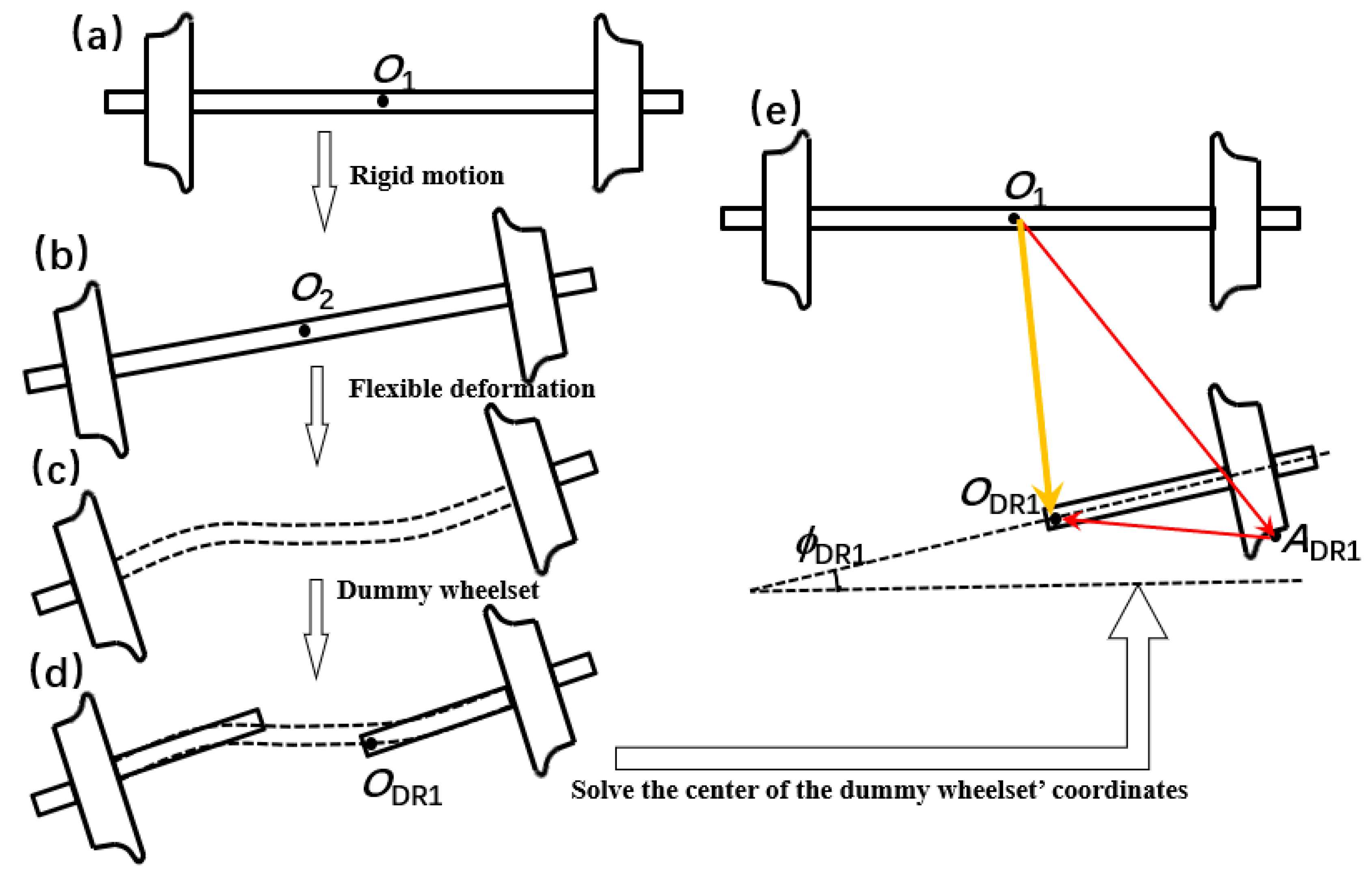
The bending deformation of the wheelset indicates that the wheel rim has hardly any deformation compared to the wheel tread when the wheelset generates bending deformation within the range of 800 Hz. This feature can be used to help solve the interaction between the geometrical position of the wheel–rail. “The method for online searching wheel-rail contact points” is used to determine the contact geometry relation between a flexible wheelset and a pair of rails [21]. The process is shown in Figure 9. The motion of the flexible wheelset includes a rigid motion and flexible deformation (Figure 9a,b). Then, a dummy wheelset is used to simulate the flexible wheelset (Figure 9c,d). The centre of the dummy wheelset’s coordinates needs to be identified, and the contact geometry relation between the dummy wheelset and the two rails can then be solved by using the trace method. Therefore, solving the problem of the flexible wheelset in rolling contact with the two rails can be transformed effectively into solving the motion of the rigid wheelset.
The most important part of solving the flexible wheelset motion is determining the centre of the dummy wheelset’s coordinates. From Figure 9e, the displacement vector of the centre of the dummy wheelset is written as:
where denotes the displacement vector of the nominal contact point in the natural system of coordinates after the wheelset generates rigid motion and flexible deformation. denotes the displacement vector from the centre of the dummy wheelset to the nominal contact point.
where is the horizontal distance between the centre of the dummy wheelset and the nominal rolling circle, is the radius of the nominal rolling circle, is the displacement vector of the contact point after the wheelset produces flexible deformation, and it can be solved using the method described in Section 3.1. ϕr denotes the angle of roll after the wheelset generates rigid motion and ψr indicates the angle of yaw. The two parameters can be solved using a dynamic explicit integral algorithm. In addition, the transformation matrix between the natural system of coordinates and the wheelset system of coordinates is built using ϕr and ψr.
is written as
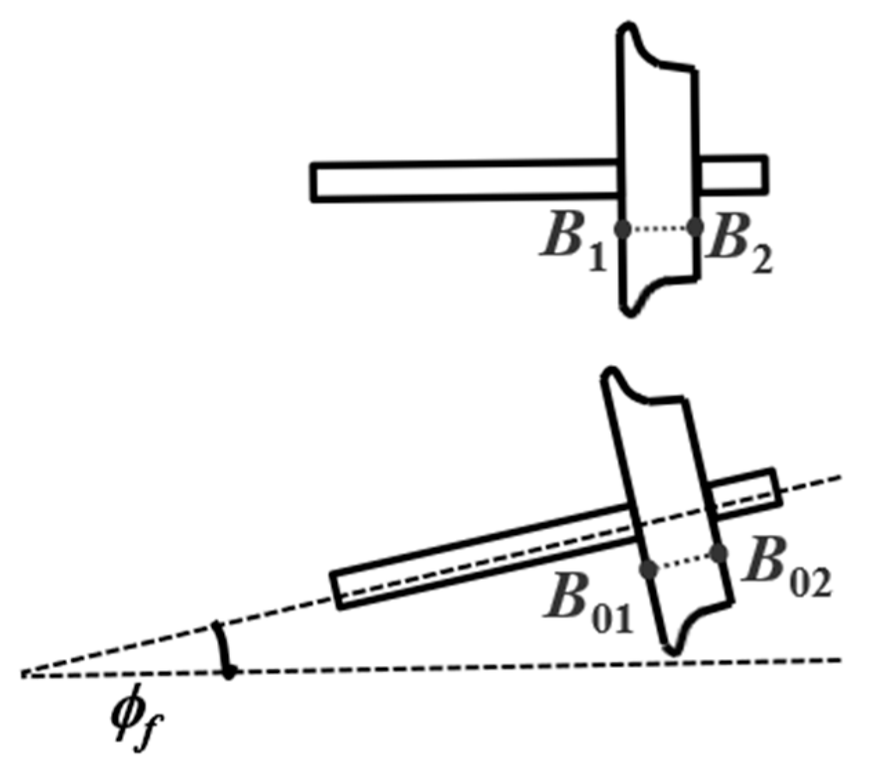
where ϕDR1 indicates the angle included between the axis of the wheelset and the horizontal line after the wheelset generates rigid motion and flexible deformation. This is written as
where ϕf denotes the angle included between the axis of the wheelset and the horizontal line after the wheelset only produces flexible deformation. Figure 10 illustrates the solving method. First, two points (B1 and B2) at both sides of the wheel are selected, and the connection line between the two points is drawn, and this line is parallel to the axis of the wheelset. Second, the wheelset generates flexible deformation, the two points move to the two new points B01 and B02. Then, the positions of B01 and B02 are solved using the method described in Section 3.1. Finally, ϕf can be solved.
In the plane perpendicular to the rails, the displacement vector of the centre of the dummy wheelset can be written as:
Then, the motion of the flexible wheelset can be determined by solving the motion of the rigid wheelset. The contact geometry relationship between the dummy wheelset and the pair of rails can be obtained by using such a trace method. The wheel–rail normal force can be calculated using the nonlinear Hertzian contact model, and the wheel–rail tangential force is calculated using Shen’s theory. For details, please refer to [13].
3.3. Archard Wear Model
The Archard wear model is used to calculate the wear loss in the contact patch; the wear loss is written as:
where is the wear loss in the contact patch, N is the normal contact force, d is the sliding distance, H is the hardness, and is the friction coefficient.
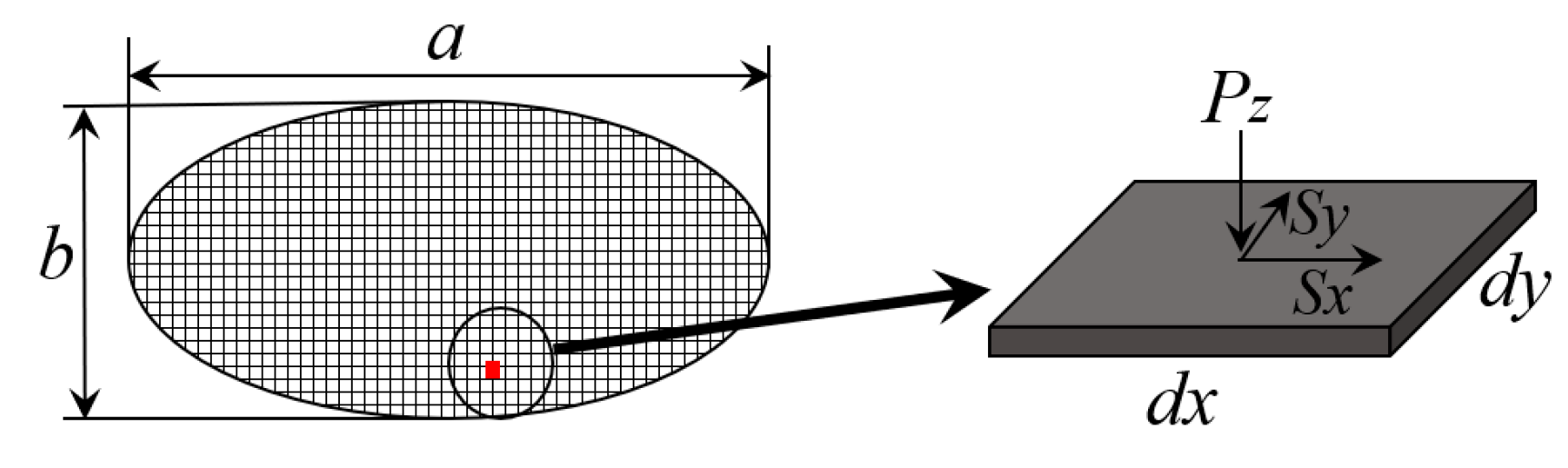
The contact patch can be divided into many elements of equal size (Figure 11), and the length and width of the element are, respectively, and . is the normal force on the element, is the lengthwise sliding velocity, is the lateral sliding velocity, and a and b are the semi major axis and the semi minor axis of the contact patch, respectively.
For an element of the contact patch, the wear loss is:
The normal force on the element is:
The sliding displacement is:
where denotes the velocity of the contact patch. Combining Equations (10)–(12), the wear loss of any elements of the contact patch can be written as:
where (x, y) is the position of the element of the contact patch. If the velocity component caused by the flexible deformation is ignored, Equation (13) is expressed as:
If the rolling contact patch is assumed to have a slight local slip, it implies , and thus, Equation (14) is expressed as:
where is the longitudinal creepage, is the lateral creepage, and is the spin creepage. These parameters can be calculated using the vehicle–track rigid–flexible coupling dynamical model. Equation (15) indicates that the wear loss of the contact patch depends on the normal force and creepages. When the distribution of these parameters along the wheel circumference fluctuates, the wear loss distribution along the wheel circumference also fluctuates, and it can easily lead to polygonal wear under certain conditions.
Selecting the wear coefficient () is important for accurately calculating the wear that occurs on the wheel–rail because of their interaction. In [24], the authors constructed the friction coefficient based on the normal contact compressive stress and sliding velocity between the wheel and the rail obtained through tests. The wear coefficient within the range of 0.0001 to 0.001 means slight wear. In this paper, is 0.0004.
Using the model discussed above to calculate polygonal wear, for simplicity, the contact points are considered to be distributed along the rolling circle of the wheel between the two adjacent contact points discretely. At these contact points, the normal load and slips of wheel–rail are calculated using the rigid–flexible coupling dynamical model of vehicle–track, discussed above. At each contact point, the wear depth of elements is calculated in the contact patch using the known normal load and slips of the wheel–rail. Then, the wear depths along the rolling circle of the wheel are summed. This process is repeated 50 times. Finally, the maximum of the summated wear size along the rolling circle of the wheel is considered as the polygonal wear depth after the wheel rolls 50 times. Because the distance between the first and last contact points is not equal, the calculated accumulative wear curve, which indicates polygonal wear discontinues, does not fit the actual scenario. A fitting method is applied to solve this problem; however, due to space limitations, this is not discussed in this paper.
4. Discussion on the Calculated Results of High-Order Polygonal Wear
Wheels with different diameters have different wavenumbers of high-order polygonal wear; however, their exciting frequencies are the same and, in general, they are in the range of 570–580 Hz (as shown in Section 2). The wheelset discussed has a bending mode of 576 Hz (as shown in Section 3.1). It is obvious that the modal frequency is close to the exciting frequency of the polygonal wear at 300 km/h. An experimental analysis of the mechanism of high-order polygonal wear of high-speed trains was conducted [12]; in that study, the authors suggested that the mechanism of polygonal wear is attributed to the excited resonance of the train–track coupling system in operation through the field tests. Therefore, the mechanism of the polygonal wear should be further investigated by developing the simulation model that involves the flexible deformation (bending deformation) of the wheelset in this paper.
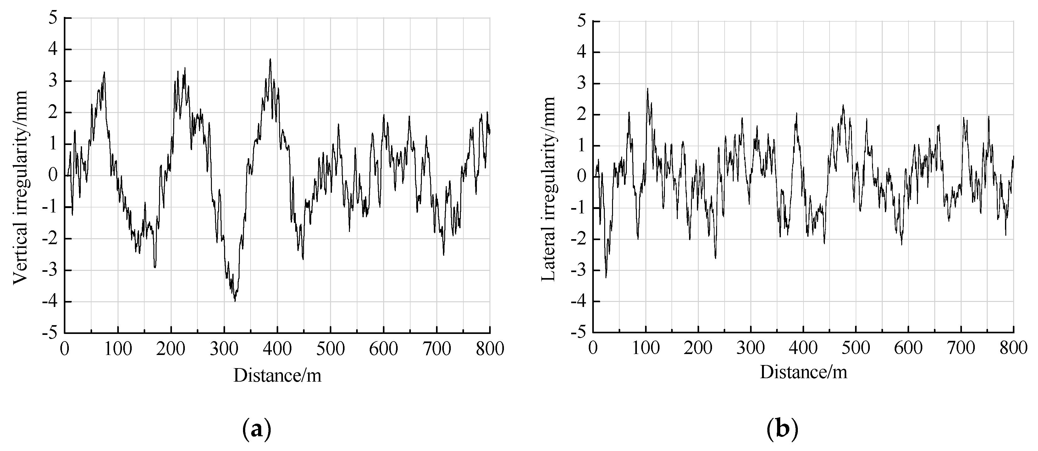
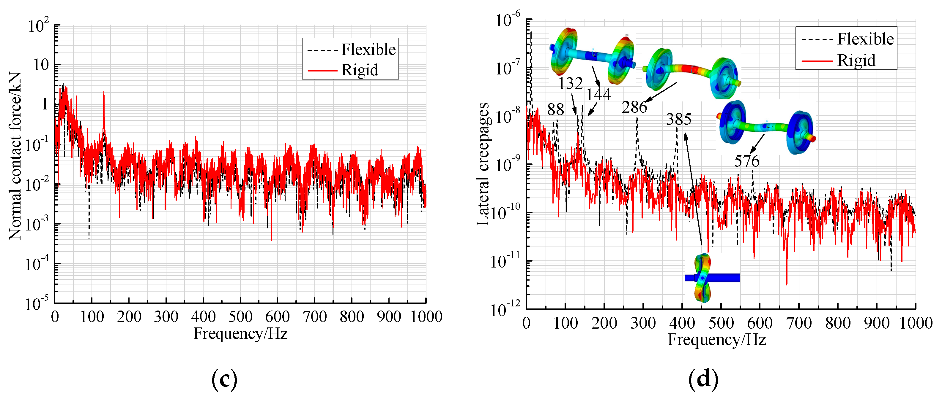
The numerical simulation uses the vehicle–track rigid–flexible coupling dynamical model described in Section 3.1, and the track random roughness is used as an exciting input (Figure 12a,b). The speed of the train is 300 km/h and the diameter of the wheel is 920 mm. The normal contact forces and creepages are calculated. Figure 12c,d shows the comparisons of the calculated results for the flexible wheelset and the rigid wheelset in the frequency domain.
As shown in Figure 12c, the normal force of the flexible wheelset is slightly smaller than that of the rigid wheelset in the considered frequency domain. The difference between the normal forces of the two types of wheelset models is relatively large at 132 Hz, which is the sleeper passing frequency. Figure 12d shows the obvious peaks of the lateral creepages at approximately 88, 132, 144, 286, 385, and 576 Hz, and there are large differences between the flexible and rigid wheelset at these frequencies. The flexible wheelset modes of 88, 144, 286, 385, and 576 Hz need to have remarkable contribution to the polygonal wear corresponding to the peaks. However, the tested results in Section 1 show that the dominant polygonal wear are in the 18th to 20th order, which are related to 576 Hz. Therefore, the numerical simulation of the present paper focuses on the influence of the wheelset vibration mode of 576 Hz only and the other modes (88, 144, 286, and 385 Hz) are excluded in the simulation program when calculating polygonal wear.
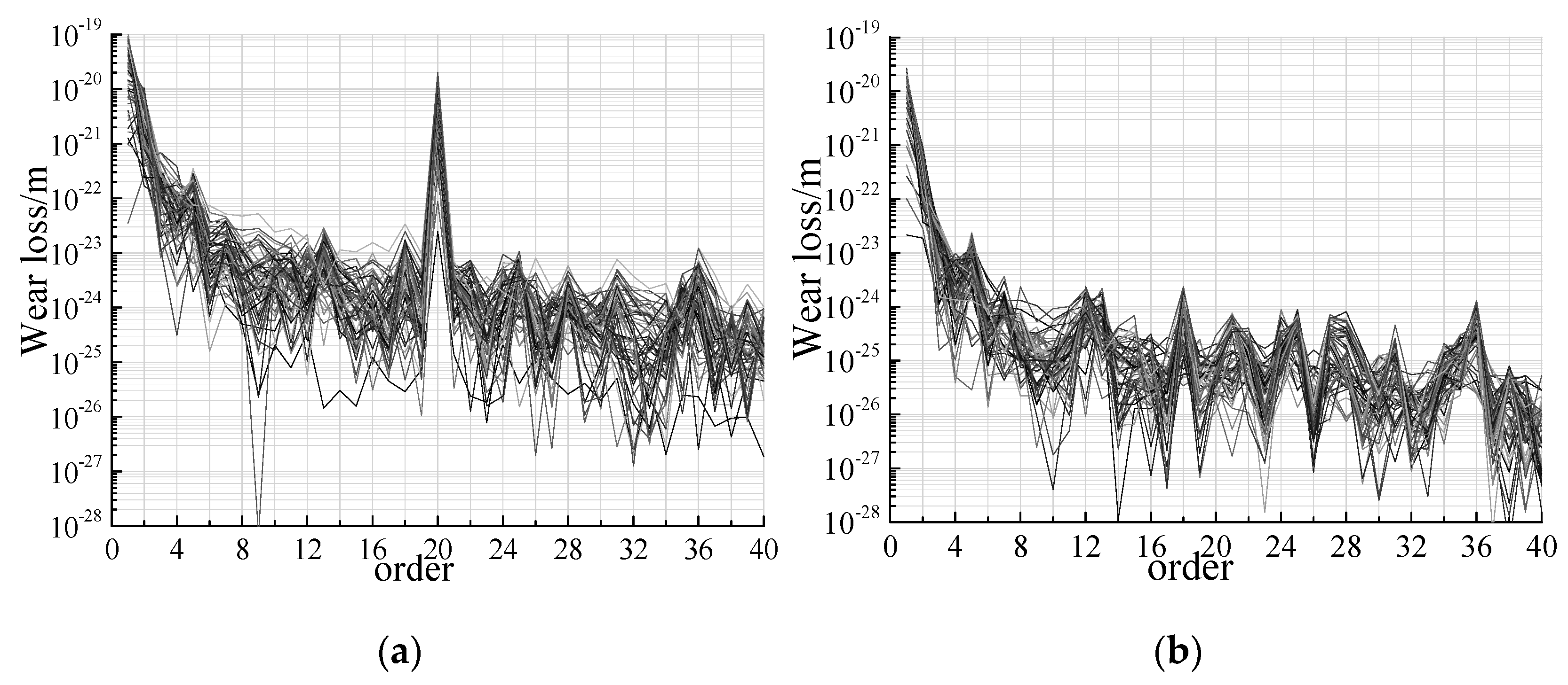
The wear model described in Section 3 is used to calculate the wear loss along the circumference of the wheel with 50 circles rolling. In the calculation, the track random roughness is used as an exciting input. Figure 13a,b show the calculated results of the wear loss along the circumferences of the two wheels with 50 rolling circles. One is a flexible wheelset and the other is a rigid wheelset. Figure 14a,b indicate their irregularity spectra corresponding to Figure 13a,b, respectively. From the calculated result, it is found that the flexible deformation of the wheelset either greatly contributes or leads to polygonal wear generation.
Note that Figure 12d shows the peaks of the lateral creepage at 88, 132, 144, 286, 385, and 576 Hz. Furthermore, the wheel circumference is approximately within the integral multiples of the wavelengths of the vibration at 144, 286, and 576 Hz, at 300 km/h and at the 920 mm wheel diameter. This is a basic condition for the generation of polygonal wear at 144, 286 and 576 Hz. The polygonal wear of the corresponding 5th, 10th, and 20th orders should start at the same time and develop quickly. However, the calculated result, as shown in Figure 14a, does not show the polygonal wear of the 5th and 10th orders. It is apparently contradictory when comparing Figure 12d with Figure 14a. In fact, the polygonal wear of 5th and 10th orders can contribute prominently if all bending modes of the wheelset are considered for calculating polygonal wear. However, the test results, as shown in Figure 15, indicate the dominant order of only 20, and its corresponding passing frequency is close to 576 Hz at a speed of 300 km/h and at a diameter close to 920 mm.
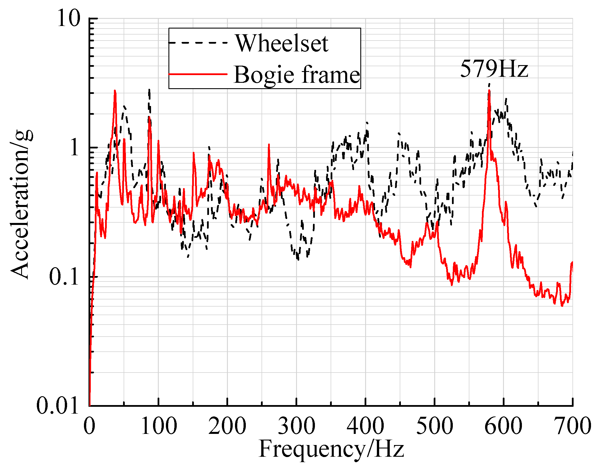
Figure 15 shows the typical site test results. Figure 15 shows the lateral vibration acceleration spectra of the wheelset bearing box and bogie frame above the primary suspension when the train is running at 300 km/h after wheel re-profiling (no polygonal wear exists). The result of the wheelset indicates that, in the actual running condition, the vibration level of the wheelset in the frequency band of 550–600 Hz is more significant than that in other frequency bands. This implies that the mode of the wheelset at 576 Hz is excited when the train is running. Furthermore, Figure 15 shows that the vibration of the bogie frame at ~579 Hz (close to a wheelset mode frequency of 576 Hz) is as dominant as that of the wheelset. In such a scenario, the 20th-order polygonal wear was initiated and developed quickly. Then, at frequencies of ~144 Hz and 286 Hz, the uncoupling vibration of the wheelset and bogie probably occurred, or other resonances at frequencies near them occurred, as shown in Figure 15. This situation could disturb or suppress the polygonal wear of the 5th and 10th orders. However, this is conjecture that can be verified by improving the present theoretical model. The current model cannot account for the effect of the bogie resonances and the frequency dependent characteristics of the suspension. Thus far, to emphasise the influence of the wheelset mode of 576 Hz, the effect of other modes was intentionally neglected in the calculation using the less advanced model.
5. Key Conditions of Initiation and Development of Polygonal Wear
5.1. Integral Multiple Condition
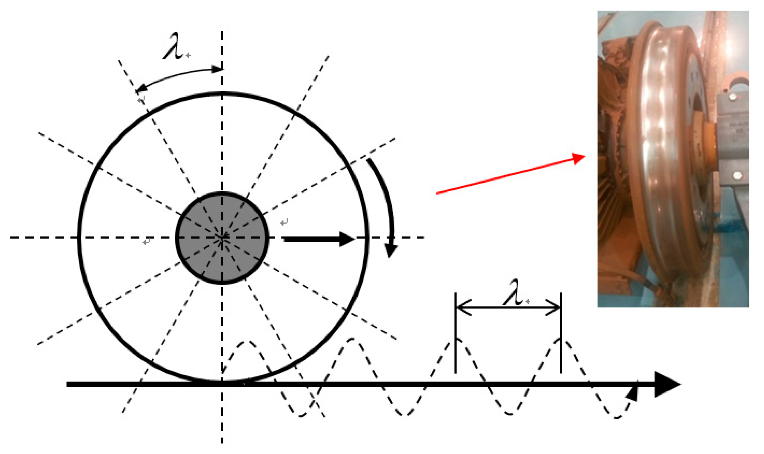
The research results show that periodically fluctuating creepage (or slip) can lead to the initiation and development of polygonal wear, and the resonance of the coupling system of train and track can cause periodically fluctuating load and creepage of the wheel–rail. If the circumference of the wheel is nearly an integral multiple of the wavelength of the excited system resonance, it is regarded as a key condition for initiating the high-rate development of polygonal wear. This is called an integral multiple condition. As shown in Figure 16 [12], the basic condition for wheel polygonal wear generation is more rigorous than that for rail corrugation formation because the rail is infinitely long and the corrugation in its development can extend infinitely along with its track. However, the perimeter of the rolling wheel is finite, and uneven wear along the wheel circumference will be superimposed circularly. The referenced start points of the uneven wear on the wheel running surface when the wheel rolls have different phases if the perimeter cannot be divided exactly by the wavelength of the uneven wear caused by the resonance. If so, the uneven wear or wheel polygonal wear develops very slowly. In the other case, wheel polygonal wear can develop very quickly. This case indicates that the changes in wheel perimeter because of the wear and re-profiling is nearly an integral multiple of the wavelength λ of the excited resonance of the wheel–rail system.
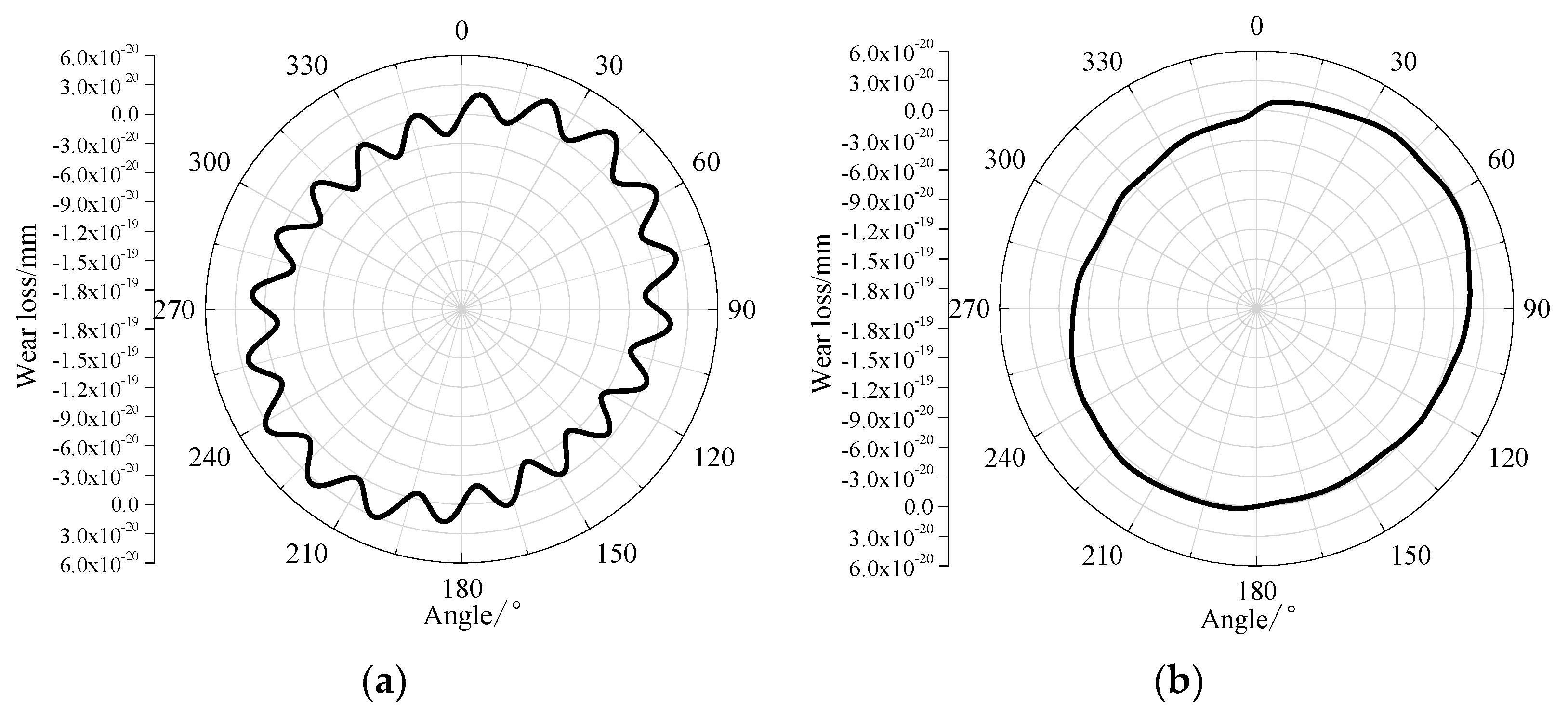
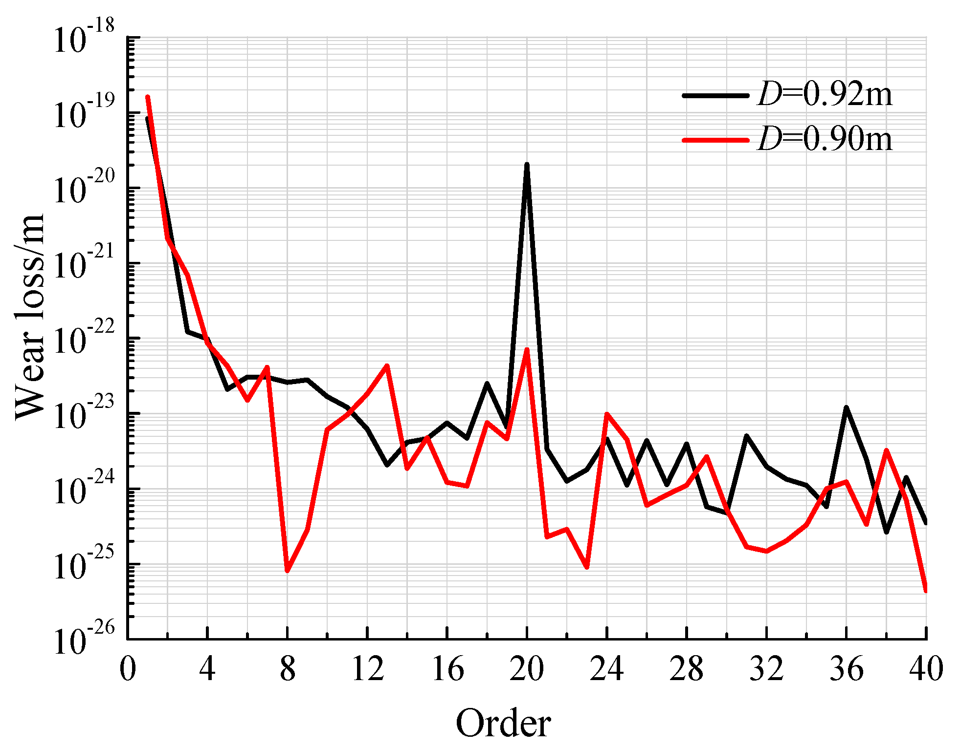
In the following analysis case, the effect of the wheelset mode of 576 Hz on the development of polygonal wear was analysed under conditions where the operating speed was 300 km/h and the wheel diameter was 900 mm and 920 mm. Figure 17 shows the effect of the diameter difference. When the wheel had a 900 mm diameter at 300 km/h, its circumference was not an integral multiple of the wavelength (v = 300 km/h and f = 576 Hz), and when the wheel had a 920 mm diameter, at 300 km/h, the integral multiple condition was nearly satisfied. Thus, the calculated wear loss along the circumferences of the two wheels with 50 rolling cycles showed a large difference at the 20th order of polygonal wear, as shown in Figure 17.
As shown in Figure 17, 20th order polygonal wear occurs on wheels with two different diameters. However, it is obvious that polygonal wear is more serious on the wheel with a diameter of 920 mm, that satisfies the integral multiple condition nearly.
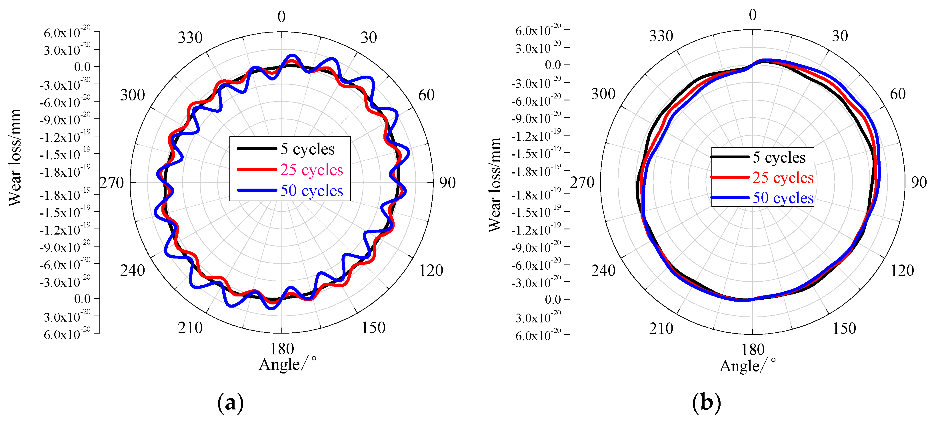
Figure 18 shows the polygonal wear results obtained by superposing the uneven wear at different wheel rolling cycles (5 cycles, 25 cycles, and 50 cycles). Figure 18a,b indicates the results of the wheels with diameters of 920 mm and 900 mm, respectively. As shown in Figure 18a, it is obvious that the wear loss along the circumference with a wear superposition of different cycles has nearly the same phase, and the polygonal wear increased gradually and rapidly. As shown in Figure 18b, for a wheel with a diameter of 900 mm, the polygonal wear does not increase considerably, and it appears similar to the polygonal wear pattern of each cycling “rotating’’ or “shifting’’ around the circumference. Superposing the uneven wear of each cycling with different initial phases eliminates their peaks and valleys. This is because the referenced start points of the uneven wear at each rolling cycle have different phases if the perimeter is not an integral multiple of the wavelength of the uneven wear. If so, the polygonal wear develops very slowly.
The wheel diameter is an important parameter that can determine whether the wheel satisfies the integral multiple condition. In addition, in the long-time service of a wheel, its diameter changes over a large range because of wear and re-profiling. Considering a high-speed train of China as an example, the diameter for its new wheel is 920 mm. The diameter of the wheel reduces to about 830 mm at the end of its use life under normal use. Therefore, several special values of the diameter during the normal use life can satisfy the integral multiple condition at 300 km/h, and then, the high-order polygonal wear occurs easily and quickly at these diameter values. For the research object in this paper, when the wheel diameters were 920 mm, 875 mm, and 830 mm, the wheels satisfied the integral multiple condition. Thus, wheels with different diameters have different proportions of polygonal wheels and different dominant polygonal orders.
5.2. Effect of Different Diameters and Different Speeds
The train is operated at different speeds v on different track lines, and the excited resonance frequency that influences the polygonal wear development does not vary considerably in the analysis during the field tests. Therefore, the operating speed determines the wavelength λ of the polygonal wear, and the integral multiple condition determines the initiation and high-rate development of polygonal wear. Therefore, the high-rate development of the polygonal wear depends on the operation speed and wheel diameter.
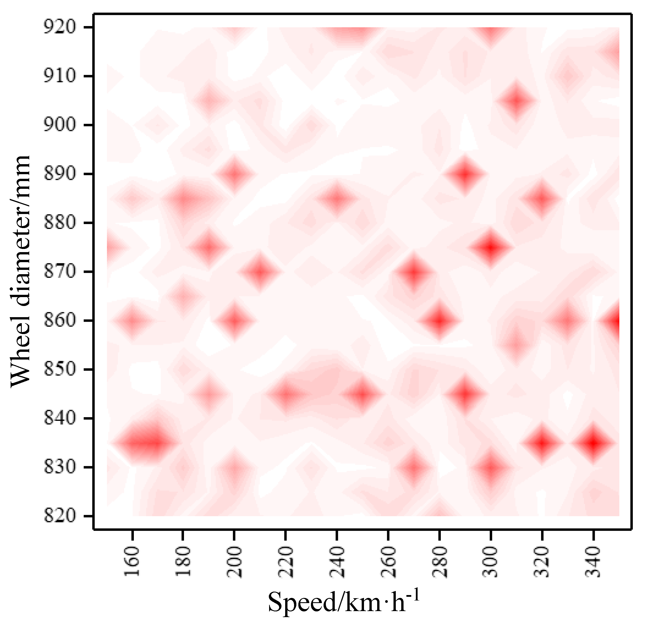
The analysis of polygonal wear development during the entire normal use life of the wheel was conducted for the following case. The analysis involves different wheel diameters, different operation speeds, and excited resonance frequencies related to the polygonal wear development at a high rate. In this analysis, the diameter was from 820 to 920 mm, the speed was from 150 to 350 km/h, and the excited resonance frequency was 576 Hz, which was assumed to refer to the test results discussed above. For the other excited resonance frequencies, a similar analysis can be conducted. The calculated wear loss along the circumference of the wheel (50 rolling cycles) with different diameters and different speeds is shown in Figure 19. In the figure, the dark areas indicate severe polygonal wear or polygonal wear development at a high rate. Special diameters that would lead to severe polygonal wear are different if the operating speeds are different. At the same speed, there are several special diameters at which the polygonal wear develops fast. Therefore, with the help of numerical results, high-rate polygonal wear development can be predicted theoretically, and the re-profiling rule of polygonal wheels can be built up easily. For example, for a train at an operating speed of 350 km/h, there are two special diameters—860 and 915 mm—at which there are dark areas (Figure 19). Therefore, after the new wheels are placed into operation in the initial stage where the diameter is ~915 mm, polygonal wear occurs; however, it is not considerably serious. The wheel diameter decreases to ~860 mm because of wear and re-profiling, and because another dark area is generated. Thus, it implies that this is a time for high-rate polygonal wear development. The corresponding wheel diameter is the “special diameter.” This time, polygonal wheels need to be re-profiled in time, or the re-profiling interval should be changed, or the train operation speed is changed considerably to decrease the fast development of polygonal wear. For any new type of high-speed train to be placed into commercial operation, the easily excited resonant frequencies related to the initiation of the polygonal wear should be known, and then, figures similar to Figure 19 can be drawn and analysed.
6. Conclusions
In this study, the characteristics of polygonal wear measured from a large number of wheels of high-speed trains were statistically analysed, and a prediction model of polygonal wear of high-speed trains was developed. Using the prediction model, the causes and the conditions of the initiation and development of the polygonal wear were studied. The main conclusions are given below.
- The prominent feature of polygonal wear is that the dominant order and development rate of polygonal wear are very closely related to the wheel diameter, operation speed, and the resonance frequencies of the system, such as wheelsets.
- If the wheel circumference is nearly an integral multiple of the wavelength of the periodical wear along the rolling circle of the wheel, the polygonal wear initiates and develops very quickly. This is referred to as the integral multiple condition, which is a key or basic condition for polygonal wear. This “integral multiple” is on the order of the dominant polygonal wear.
- When the excited resonance frequency of the vehicle system is determined to be related to polygonal wear, the initiation and development of the polygonal wear depends on the operation speed and wheel diameter. Their relationship diagram is provided, and it can be used to predict polygonal wear development, modify the re-profiling schedule of polygonal wheels, and eliminate the polygonal wear on the wheels in time.
- The effect of flexibility of the wheelset is considered in the prediction model of the polygonal wear of high-speed wheels in this paper. Therefore, the high-frequency characteristics of the wheelset bending resonances can be more accurately expressed, and high-order polygonal wear related to the wheelset bending resonances at high frequencies can be numerically reproduced.
However, the current simulation model can only reflect the actual scenario of the train to a certain extent, and some phenomena cannot be accurately reflected. In addition, it cannot account for the effect of the bogie resonances and the frequency dependent characteristics of the suspension. In short, the current simulation model needs to be improved further.
Author Contributions
Conceptualization, Y.W. and X.J.; methodology, Y.W., J.H., and W.C.; validation, Y.W., X.X., and X.J.; investigation, Y.W.; writing—original draft preparation, Y.W.; writing—review and editing, X.J.; supervision, X.J.; project administration, X.J.; funding acquisition, X.J. All authors have read and agreed to the published version of the manuscript.
Funding
This research was funded by the National Science Foundation of China, grant numbers U1734201 and 51805450.
Acknowledgments
The authors wish to thank CSR Tangshan Rolling Stock Co., Ltd. for their assistance in conducting the experiment. We also would like to thank Editage for English language editing.
Conflicts of Interest
The authors declare no conflict of interest.
Appendix A
The shape testing of all elements is conducted to ensure that a sufficiently fine mesh has been used. The summary of the shape testing is listed in Table A1.

Table A1.
The summary of the shape testing.
| Test Items | Number Tested | Warning Count | Error Count | Warn+Err (%) |
|---|---|---|---|---|
| Aspect Ratio | 255,360 | 5232 | 0 | 2.05% |
| Parallel Deviation | 255,360 | 0 | 0 | 0 |
| Maximum Angle | 255,360 | 0 | 0 | 0 |
| Jacobian Ratio | 255,360 | 0 | 0 | 0 |
| Warping Factor | 255,360 | 0 | 0 | 0 |
In order to ensure that the selected mesh size has little effect on the results of modal analysis, the two new finite element models with smaller element size were built, as shown in Figure A1. The comparison results of modal analysis are shown in Table A2.
Figure A1.
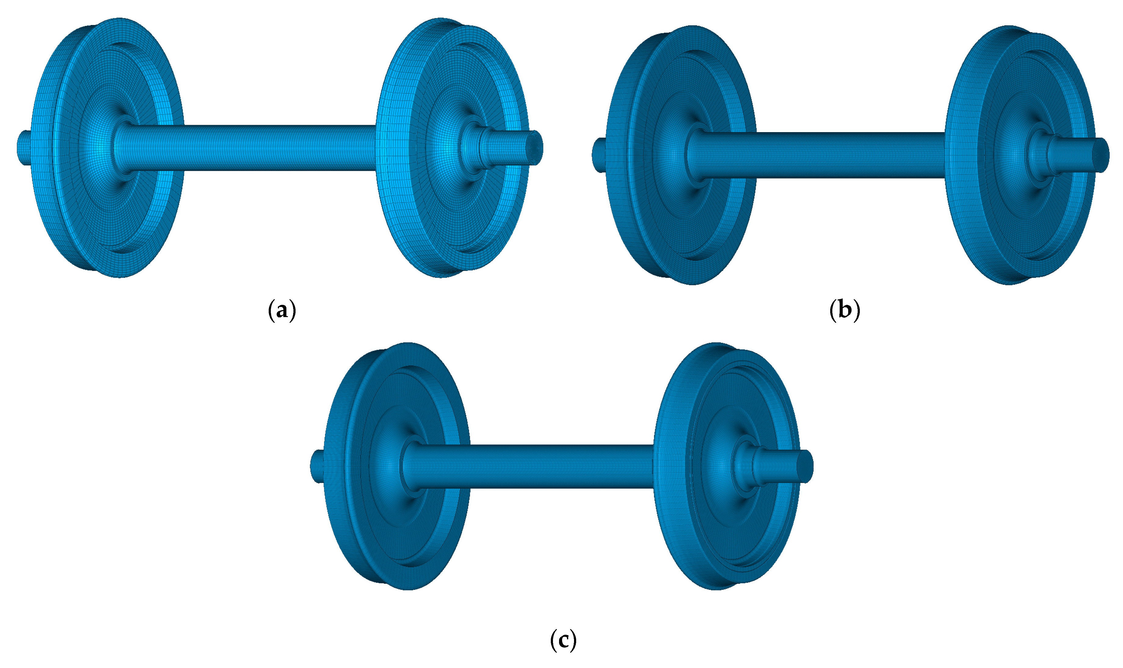
The finite element model: (a) Model 1 (the model in the manuscript, element count: 255,360, node count: 267,771); (b) Model 2 (element count: 556,800, node count: 573,673); (c) Model 3 (element count: 834,860, node count: 856,285).
Figure A1.
The finite element model: (a) Model 1 (the model in the manuscript, element count: 255,360, node count: 267,771); (b) Model 2 (element count: 556,800, node count: 573,673); (c) Model 3 (element count: 834,860, node count: 856,285).

Table A2.
The comparison results of modal analysis.
| Model 1 (the Model in the Manuscript) | Model 2 | Model 3 | |||
|---|---|---|---|---|---|
| Element count | 255,360 | 556,800 | The errors refer to model 1 (%) | 834,860 | The errors refer to model 1 (%) |
| Node count | 267,771 | 573,673 | 856,285 | ||
| Order | Frequency | ||||
| 1 | 72.13 | 72.12 | 0.01% | 72.12 | 0.01% |
| 2 | 87.08 | 87.02 | 0.07% | 86.95 | 0.15% |
| 3 | 143.6 | 143.3 | 0.21% | 142.9 | 0.49% |
| 4 | 234.1 | 233.3 | 0.34% | 232.1 | 0.85% |
| 5 | 284.7 | 284.0 | 0.25% | 283.2 | 0.53% |
| 6 | 347.3 | 346.1 | 0.35% | 344.1 | 0.92% |
| 7 | 386.0 | 385.4 | 0.16% | 384.9 | 0.28% |
| 8 | 576.4 | 575.7 | 0.12% | 574.7 | 0.29% |
References
- Johansson, A. Out-of-round Railway Wheels—Literature Survey, Field Tests and Numerical Simulations. Licentiate Thesis, Chalmers University of Technology, Göteborg, Sweden, 2003. [Google Scholar]
- Jin, X.S.; Wu, Y.; Liang, S.L.; Wen, Z.F. Advance in research on mechanism of out-of-roundness wear of railway vehicle wheels and its solution countermeasure. J. Southwest Jiaotong Univ. 2018, 53, 1–14. [Google Scholar]
- Nielsen, J.C.O.; Johansson, A. Out-of-round railway wheels—A literature survey. Proc. Inst. Mech. Eng. F J. Rail Rapid Transit 2000, 214, 79–91. [Google Scholar] [CrossRef]
- Kaper, H.P. Wheel corrugation on Netherlands railway (NS): Origin and effects of ‘polygonization’ in particular. J. Sound Vib. 1998, 120, 267–274. [Google Scholar] [CrossRef]
- Morys, B.; Kuntze, H.B.; Hirsch, U. Investigation of origin and enlargement of out-of-round phenomena in high speed ICE-wheelsets. In Proceedings of the 10th European ADAMS Users’ Conference, Frankfurt, Germany, 14–15 November 1995; Volume 14, p. 1. [Google Scholar]
- Morys, B.; Kuntze, H.B. Simulation analysis and active compensation of the out-of-round phenomena at wheels of high speed trains. In Proceedings of the World Congress on Railway Research, Florence, Italy, 16–19 November 1997. [Google Scholar]
- Morys, B. Enlargement of out-of-round wheel profiles on high speed trains. J. Sound Vib. 1999, 227, 965–978. [Google Scholar] [CrossRef]
- Meinke, P.; Meinke, S.; Szoc, T. On dynamics of rotating wheel/rail systems in a medium frequency range. In Proceedings of the 4th German-Polish Workshop Dynamical Problems in Mechanical Systems, Warszawa, Poland, 30 July–4 August 1996. [Google Scholar]
- Meywerk, M. Polygonalizaiton railway wheels. Arch. Appl. Mech. 1999, 69, 102–120. [Google Scholar] [CrossRef]
- Chen, G.X.; Jin, X.S.; Wu, P.B.; Dai, H.Y.; Zhou, Z.R. Finite element study on the generation mechanism of polygonal wear of railway wheels. J. China Railw. Soc. 2011, 33, 14–18. [Google Scholar]
- Tao, G.; Wang, L.; Wen, Z.; Guan, Q.; Jin, X. Measurement and assessment of out-of-round electric locomotive wheels. Proc. Inst. Mech. Eng. F 2016, 232, 275–287. [Google Scholar] [CrossRef]
- Tao, G.; Wang, L.; Wen, Z.; Guan, Q.; Jin, X. Experimental investigation into the mechanism of the polygonal wear of electric locomotive wheels. Veh. Syst. Dyn. 2018, 56, 1–17. [Google Scholar] [CrossRef]
- Jin, X.; Wu, L.; Fang, J.; Zhong, S.; Ling, L. An investigation into the mechanism of the polygonal wear of metro train wheels and its effect on the dynamic behaviour of a wheel/rail system. Veh. Syst. Dyn. 2012, 50, 1817–1834. [Google Scholar] [CrossRef]
- Wu, Y.; Du, X.; Zhang, H.J.; Wen, Z.F.; Jin, X.S. Experimental analysis of the mechanism of high-order polygonal wear of wheels of a high-speed train. J. Zhejiang Univ. Sci. A 2017, 18, 579–592. [Google Scholar] [CrossRef]
- Wu, X.; Rakheja, S.; Cai, W.; Chi, M.; Ahmed, A.; Qu, S. A study of formation of high order wheel polygonalization. Wear 2019, 424, 1–14. [Google Scholar] [CrossRef]
- Cai, W.; Chi, M.; Tao, G.; Wu, X.; Wen, Z. Experimental and numerical investigation into formation of metro wheel polygonalization. Shock Vib. 2019, 2019, 1–18. [Google Scholar] [CrossRef]
- Zhai, W.M. Vehicle-Track Coupled Dynamics, 4th ed.; Science Press: Beijing, China, 2007. [Google Scholar]
- Zhong, S.; Xiong, J.; Xiao, X.; Wen, Z. Effect of the first two wheelset bending modes on wheel-rail contact behavior. J. Zhejiang Univ. Sci. A 2014, 15, 984–1001. [Google Scholar] [CrossRef]
- Xiao, X.B.; Ling, L.; Jin, X.S. A study of the derailment mechanism of a high-speed train due to an earthquake. Veh. Syst. Dyn. 2012, 50, 449–470. [Google Scholar] [CrossRef]
- Han, J.; Zhong, S.Q.; Xiao, X.B.; Wen, Z.F.; Zhao, G.T.; Jin, X.S. High-speed wheel/rail contact determining method with rotating flexible wheelset and validation under wheel polygon excitation. Veh. Syst. Dyn. 2018, 56, 1233–1249. [Google Scholar] [CrossRef]
- Li, L.; Xiao, X.B.; Jin, X.S. Interaction of subway LIM vehicle with ballasted track in polygonal wheel wear development. Acta Mech. Sin. 2011, 27, 297–307. [Google Scholar] [CrossRef]
- Ling, L.; Xiao, X.B.; Xiong, J.Y.; Zhou, L.; Wen, Z.F.; Jin, X.S. Erratum to: A 3D model for coupling dynamics analysis of high-speed train/track system. J. Zhejiang Univ. Sci. A 2015, 15, 964–983. [Google Scholar] [CrossRef] [Green Version]
- Han, J.; Zhong, S.Q.; Zhou, X.; Xiao, X.B.; Zhao, G.T.; Jin, X.S. Time-domain model for wheel-rail noise analysis at high operation speed. J. Zhejiang Univ. Sci. A 2017, 18, 593–602. [Google Scholar] [CrossRef]
- Jendel, T. Prediction of Wheel Profile Wear-methodology and Verification. Licentiate Thesis, Department of Vehicle Engineering, KTH, Stockholm, Sweden, 2000. [Google Scholar]
Figure 1.
(a) Test instrument; (b) Polygonal wheel.

Figure 2.
Statistical results of polygonal wheels.

Figure 3.
Sketch map: Amplitude spectrum of polygonal wear (site measurement) and threshold line of high-speed wheel roughness (referring to the ISO-3095).
Figure 3.
Sketch map: Amplitude spectrum of polygonal wear (site measurement) and threshold line of high-speed wheel roughness (referring to the ISO-3095).

Figure 4.
Results of the measured polygonal wear.

Figure 5.
Polygonal wear of different orders corresponding to different wheel diameters.

Figure 6.
Decrease in order with a decrease in wheel diameter.

Figure 7.
Vehicle–track rigid–flexible coupling dynamical model.

Figure 8.
Bending modes of wheelset (0–800 Hz): (a) First bending mode at 87 Hz; (b) Second bending mode at 143 Hz; (c) Third bending mode at 284 Hz; (d) Fourth bending mode at 576 Hz.
Figure 8.
Bending modes of wheelset (0–800 Hz): (a) First bending mode at 87 Hz; (b) Second bending mode at 143 Hz; (c) Third bending mode at 284 Hz; (d) Fourth bending mode at 576 Hz.

Figure 9.
Modelling flexible wheelset: (a) Static wheelset; (b) The wheelset after rigid motion; (c) The wheelset after flexible deformation; (d) dummy wheelsets; (e) the contact geometry relation between the dummy wheelset and the two rails.
Figure 9.
Modelling flexible wheelset: (a) Static wheelset; (b) The wheelset after rigid motion; (c) The wheelset after flexible deformation; (d) dummy wheelsets; (e) the contact geometry relation between the dummy wheelset and the two rails.

Figure 10.
Solving method of .

Figure 11.
Forces on elements of contact patch.

Figure 12.
(a) Vertical irregularity; (b) Lateral irregularity; (c) Normal contact forces; (d) Lateral creepages.
Figure 12.
(a) Vertical irregularity; (b) Lateral irregularity; (c) Normal contact forces; (d) Lateral creepages.


Figure 13.
Results of wear loss along the circumferences of the two wheels with rolling of 50 circles. (a) Flexible wheelset and (b) Rigid wheelset.
Figure 13.
Results of wear loss along the circumferences of the two wheels with rolling of 50 circles. (a) Flexible wheelset and (b) Rigid wheelset.

Figure 14.
Spectra corresponding to Figure 13a,b. (a) Flexible wheelset and (b) Rigid wheelset.
Figure 14.
Spectra corresponding to Figure 13a,b. (a) Flexible wheelset and (b) Rigid wheelset.

Figure 15.
Lateral vibration acceleration spectra of the wheelset and bogie frame.

Figure 16.
Description of basic condition for wheel OOR generation [12].
Figure 16.
Description of basic condition for wheel OOR generation [12].

Figure 17.
Calculated wear loss along the circumferences of wheels with two different diameters.

Figure 18.
Polygonal wear results obtained by superposing the uneven wear of the wheels rolling with cycles, (a) D = 920 mm, (b) D = 900 mm.
Figure 18.
Polygonal wear results obtained by superposing the uneven wear of the wheels rolling with cycles, (a) D = 920 mm, (b) D = 900 mm.

Figure 19.
Polygonal wear development with different operation speeds and different wheel diameters.
Figure 19.
Polygonal wear development with different operation speeds and different wheel diameters.

Table 1.
Parameter values of the vehicle and track subsystem.
| Vehicle System | Track System | ||
|---|---|---|---|
| Parameter | Value | Parameter | Value |
| Car body mass (kg) | 44,039 | Young’s modulus of rail (N/m2) | 2.059 × 10¹¹ |
| Bogie mass (kg) | 2439 | Shear modulus of rail (N/m2) | 7.9 × 10¹⁰ |
| Wheelset mass (kg) | 1881 | Density of rail (kg/m3) | 7860 |
| Density of wheelset (kg/m3) | 7860 | Cross-sectional area (m2) | 7.745 × 10⁻³ |
| Primary suspension vertical stiffness (MN/m) | 9 | Bending moment about y-axis (m4) | 3.217 × 10⁻⁵ |
| Primary suspension vertical damping (kN·s/m) | 10.5 | Bending moment about z-axis (m4) | 5.26 × 10⁻⁶ |
| Primary suspension lateral stiffness (MN/m) | 5.45 | Polar moment of inertia (m4) | 3.741 × 10⁻⁵ |
| Primary suspension lateral damping (kN·s/m) | 5.0 | Lateral shear coefficient | 0.4570 |
| Secondary suspension vertical stiffness (MN/m) | 0.24 | Vertical shear coefficient | 0.5329 |
| Secondary suspension vertical damping (kN·s/m) | 25 | Density of slab (kg/m3) | 2800 |
| Secondary suspension lateral stiffness (MN/m) | 0.13 | Young’s modulus of slab (N/m2) | 3.6 × 10¹⁰ |
| Secondary suspension lateral damping (kN·s/m) | 15 | Rail pad vertical stiffness (MN/m) | 40 |
| Distance between two bogie frames (m) | 8.9 | Rail pad vertical damping (kN·s/m) | 30 |
| Wheelbase (m) | 2.5 | Sleeper spacing (m) | 0.63 |
© 2020 by the authors. Licensee MDPI, Basel, Switzerland. This article is an open access article distributed under the terms and conditions of the Creative Commons Attribution (CC BY) license (http://creativecommons.org/licenses/by/4.0/).
Share and Cite
MDPI and ACS Style
Wu, Y.; Jin, X.; Cai, W.; Han, J.; Xiao, X. Key Factors of the Initiation and Development of Polygonal Wear in the Wheels of a High-Speed Train. Appl. Sci. 2020, 10, 5880. https://doi.org/10.3390/app10175880
AMA Style
Wu Y, Jin X, Cai W, Han J, Xiao X. Key Factors of the Initiation and Development of Polygonal Wear in the Wheels of a High-Speed Train. Applied Sciences. 2020; 10(17):5880. https://doi.org/10.3390/app10175880
Chicago/Turabian StyleWu, Yue, Xuesong Jin, Wubin Cai, Jian Han, and Xinbiao Xiao. 2020. "Key Factors of the Initiation and Development of Polygonal Wear in the Wheels of a High-Speed Train" Applied Sciences 10, no. 17: 5880. https://doi.org/10.3390/app10175880
Note that from the first issue of 2016, this journal uses article numbers instead of page numbers. See further details here.