Recent Advances in Saliency Estimation for Omnidirectional Images, Image Groups, and Video Sequences


Department of Informatics, Systems and Communication, University of Milano-Bicocca, Viale Sarca 336, 20126 Milan, Italy
Appl. Sci. 2020, 10(15), 5143; https://doi.org/10.3390/app10155143
Submission received: 9 July 2020
/
Revised: 23 July 2020
/
Accepted: 24 July 2020
/
Published: 27 July 2020
(This article belongs to the Special Issue Texture and Colour in Image Analysis)
Abstract
:We present a review of methods for automatic estimation of visual saliency: the perceptual property that makes specific elements in a scene stand out and grab the attention of the viewer. We focus on domains that are especially recent and relevant, as they make saliency estimation particularly useful and/or effective: omnidirectional images, image groups for co-saliency, and video sequences. For each domain, we perform a selection of recent methods, we highlight their commonalities and differences, and describe their unique approaches. We also report and analyze the datasets involved in the development of such methods, in order to reveal additional peculiarities of each domain, such as the representation used for the ground truth saliency information (scanpaths, saliency maps, or salient object regions). We define domain-specific evaluation measures, and provide quantitative comparisons on the basis of common datasets and evaluation criteria, highlighting the different impact of existing approaches on each domain. We conclude by synthesizing the emerging directions for research in the specialized literature, which include novel representations for omnidirectional images, inter- and intra- image saliency decomposition for co-saliency, and saliency shift for video saliency estimation.
1. Introduction
Visual saliency is defined as a property of a scene in relation to an observer. This follows from a commonly-accepted interpretation [1,2,3] that defines it as the set of subjective and perceptual attributes that make certain items stand out from their surroundings, and therefore grab the viewer’s attention.
In the vision system of human beings and other animals, two components typically contribute to the overall saliency: bottom-up and top-down factors [4]. Bottom-up saliency is driven by low-level activations in the vision system, based for example on pre-attentive computational mechanisms in the primary visual cortex [5], and does not depend on specific tasks and objectives. Conversely, top-down saliency is defined as being goal-directed [6], and as such it is highly dependent on the intrinsic biases of the observer, and correlated to the semantics of the depicted elements. Scientific literature reviews for automatic visual saliency estimation often adopt these two categories to classify existing methods [2]. For example, deep learning solutions are rightfully labeled as top-down approaches due to their intrinsic ability to extract and exploit semantic pieces of information [7], whereas hand-crafted methods tend to rely on lower-level features such as contrasting patterns, and are therefore categorized as bottom-up solutions. In practice, though, multiple interacting factors (both top-down and bottom-up) are considered to determine which parts of the scenes are further processed by the attentional process of the biological vision system [8].
Properly modeling visual saliency means emulating the widest set of factors that influence the evaluation of saliency as performed by a human being. This goal has been pursued by many authors, both in the neuroscience community and, more recently, in the computer vision and image processing communities. Due to the different levels of involved complexity, bottom-up saliency estimation methods are generally faster than top-down methods [9], and thus useful in applications where real-time feedback is considered more important than reaching higher accuracy. For example, in a live augmented reality scenario, fast saliency estimation would locate image regions deemed important for further localized computer vision analysis, and would provide precious information to avoid covering areas of potential interest with the rendering of augmentation elements. Conversely, top-down saliency estimation methods tend to be more robust, at the cost of a higher demand for computational resources. These are therefore typically employed in applications with looser time constraints, and which benefit from semantic interpretation. For example, a system for storing and organizing personal photos could exploit saliency estimation to detect objects of interests based on visual composition, and their reoccurring presence in multiple photos. In general, visual saliency estimation has been successfully employed in multiple tasks, such as image retargeting [10], video summarization [11], and photo-collage creation [12]. It has also been adopted as an intermediate pre-processing step for other computer-vision problems, such as scene recognition [13], object detection [14] and segmentation [15]. Since the advent and diffusion of deep-learning, many of these problems have been reformulated in an end-to-end fashion that does not rely on explicitly estimating the salient component, as proven by state of the art solutions in each field [16,17,18]. There exist, however, problems that remain directly related to the evaluation of saliency information such as advertisement assessment [19], and domains where its explicit computation is particularly relevant, for example in reducing the computational effort for analysis of large quantities of data (such as video sequences, or high-resolution panoramic images exploited in the virtual reality domain).
By analyzing the recent scientific literature on saliency estimation, in fact, specific topics emerged as persistently reoccurring amidst works dedicated to saliency on regular images, due to a combination of the excellent results already reached by the scientific community, and the paradigm shift in solving certain problems without explicitly modeling general-purpose saliency. Such trending topics are, namely, saliency in omnidirectional images, and multiple-input scenarios, which include co-saliency and video saliency estimation. Although visual saliency has been studied in other fields as well (such as light field and hyper-spectral imaging) most of the current domain-specific research happens to converge on the three mentioned topics, while the literature does not offer enough material to produce a valuable review of recent solutions related to other less widespread domains. Our goal is therefore to highlight the recent trends of research in these fields, providing a concise yet exhaustive insight into each analyzed method, and summarizing the similarities and differences across different solutions. The investigated domains are either very recent, or have lived a particularly dynamic evolution. As a consequence, different methods are typically evaluated and/or optimized on different datasets, making comparative evaluations extremely challenging. Nonetheless, we conduct an analysis on the joint occurrence of methods and datasets, and we benchmark solutions that are directly comparable as they were evaluated in equivalent conditions.
Accompanying the development of research into visual saliency estimation through the years, the scientific literature has periodically offered different benchmarks and surveys, typically concerning general-purpose saliency. Borji et al. (2012) [20] provide an in-depth comparison of 35 state of the art methods for saliency estimation, over both synthetic and natural images. A second work by Borji et al. (2015) [9] conduct a similar benchmark including newly developed solutions, the most recent of which, however, was released in the year 2014. A more recent review is presented by Wang et al. (2019) [21], offering an in-depth survey over methods for salient object detection specifically based on deep learning approaches. Concerning domain-specific analyses, Cong et al. (2019-I) [22] cover methods for saliency detection that rely on so-called “comprehensive information”, such as depth cues, inter-image correspondence (equivalent to co-saliency), and multiple frames. Zhang et al. (2018) [23] review the concepts, applications, and challenges intrinsic into co-saliency detection, whereas Riche et al. (2016) [24] focus on video saliency estimation approaches based on a bottom-up interpretation. With the current survey, our goal is to inform on up-to-date developments in the fields of domain-specific visual saliency estimation. To the best of our knowledge, there are currently no surveys that specifically focus on saliency estimation in omnidirectional images, which is the most recent domain-specific development in the field.
The main contributions of this paper are the following:
- We highlight domains that naturally emerged from a literature review as being particularly timely and relevant.
- Through a systematic analysis of the methods in each domain, we show their commonalities and differences.
- We provide clear information regarding the targeted ground truth representation, as well as the output that each method can explicitly generate.
- We conduct, where deemed fair, a quantitative comparison of the selected methods, and provide some insights on the basis of such comparison.
- We report an in-depth analysis of the most common datasets for the analyzed domains, including the representation used for the ground truth saliency information.
- We present the commonly used evaluation measures, which can be either domain-specific or general-purpose.
- We conclude by synthesizing the emerging directions for research in the specialized literature.
The rest of the paper is structured as follows: Section 2 presents the systematic approach that led to the selection of works in this review. Section 3 introduces the three domains of interest and their peculiarities, followed by the description of different interpretations and representations commonly adopted for visual saliency, and an overview of existing metrics and measures used to assess saliency estimation algorithms. The subsequent sections present methods, datasets, and measures for each domain of interest: Section 4 focuses on omnidirectional images, Section 5 relates to co-saliency estimation, and finally, Section 6 presents developments in the field of video saliency.
2. Methodology for Literature Review
The selection of literature works included in this review paper has been determined through a systematic approach, which is described in the following.
The initial prompt was to observe and highlight the current trends in visual saliency estimation. With this objective, we performed a keyword-based search on the academic search engine Google Scholar, using the terms: “visual saliency”, “saliency estimation”, “salient object detection”. Given the time-sensitive nature of our goal, we restricted the results to works published no earlier than 2017. For each resulting paper, we retrieved the following information:
- Title
- Year of publication
- Author list
- Venue (the specific journal or conference)
- Abstract
- Number of citations
For the years 2018 and 2017, we restricted the number of results to those having collected at least one citation at the time of the review, intending to focus on the dissemination of works that are considered relevant by the scientific community. Based on the title and abstract analysis, then, we excluded some further results:
- Works that do not fit in the field of visual saliency (retrieved due to the unreliability of keyword-based search alone);
- Works that focus on extremely narrow tasks (e.g., saliency estimation for skin lesions, or for comic strips).
Works related to datasets and surveys have also been isolated and used as a reference for the corresponding sections. We annotated the remaining results in terms of domains of application, and the most recurring themes emerged as being: saliency estimation for omnidirectional images, co-saliency estimation, and saliency estimation for video sequences. We therefore focused on these domains to provide the scientific community with an analysis of relevant and recent developments. For each of the selected works, domain-specific and cross-domain characteristics have been collected through careful study of the corresponding manuscripts.
The final selection of recent and relevant methods for saliency estimation has then been used as the starting point to identify the associated evaluation measures and the associated datasets. Evaluation measures have been classified as either general-purpose (presented in Section 3.3), or domain-specific (presented in the corresponding Section 4, Section 5 and Section 6).
In virtue of the importance of data in training and assessing methods for visual saliency estimation, we dedicated for each domain an in-depth analysis of the corresponding datasets. A matrix describing the joint occurrences of datasets and methods has been defined and presented for all three domains. At this stage, no explicit constraint on the release date has been imposed: the rationale is that if a dataset is still widely adopted as a benchmark for new methods, it is to be considered relevant and worth mentioning. Multiple instances of the same dataset being reported with different names have been identified and merged. Conversely, whenever two or more saliency estimation methods refer to the same dataset in different versions, this piece of information has been annotated and reported. Finally, all datasets that were identified during the preliminary, keyword-based, search have been found to be already present in the current selection. Detailed characteristics of the identified datasets have been presented.
3. Visual Saliency Estimation
In this section, we describe the recently emerged domains for visual saliency, and provide background information about the different types of saliency representation, as well as commonly used evaluation measures.
3.1. Domains
The scientific literature on saliency estimation has witnessed the emergence of domain-specific solutions, covering a wide range of topics that go beyond the traditional regular-image input. Specifically, recent developments have shown several works in the domains of omnidirectional images, image groups for co-saliency estimation, and video sequences, as exemplified in Figure 1. Other fields of application, such as light field [25] and hyper-spectral imaging [26,27] have also caught the attention of saliency-related research. Visual saliency estimation is, however, still at its early stages in such domains, and a full review of related methods is therefore left as a future development.
Another relevant domain of research is depth-assisted visual saliency estimation, which explores the advantages of predicting saliency on so-called RGB-D images [28]. In this case, the additional knowledge associated to the distance between the camera and the depicted elements can improve the separation of subjects from the background, providing a precious piece of information for better saliency estimation. Despite the clear relevance of the topic, we chose not to explicitly discuss this domain since such a wide field deserves a whole dedicated survey paper. Nonetheless, we found that depth-assisted saliency estimation is sometimes included in the analyzed domains of omnidirectional images [29], co-saliency [30], and video saliency [31]. We will, therefore, reference and discuss only these works in the corresponding sections.
Omnidirectional images (ODIs) are panoramic representations of a scene, covering a 360° solid angle from a single viewpoint, typically employed in passive virtual reality. Virtual reality is the experience of a simulated world, which can be navigated by the user to varying degrees of freedom [32]. In a passive virtual reality scenario, the spatial movements are predefined, and the virtual environment is precomputed in a sequence of omnidirectional images. During fruition, the user only determines the direction of viewing, i.e., the subpart of the ODI to visualize at any given time. Image cropping for thumbnail selection is particularly valuable when operating on large omnidirectional images, depicting wide sceneries in high-resolution [33]. Storing and transmitting these ODIs can then benefit from perceptually-aware compression, i.e., reducing the represented detail over areas that are considered “less-interesting” [34].
Image co-saliency refers to the problem of estimating the saliency from a group of images that depict the same subject. The rationale behind this approach is to provide the saliency estimation model with additional information, and thus partially compensate for the ill-posed nature of the problem. Depending on the chosen level of abstraction, image groups for co-saliency estimation could either represent exactly the same instance from multiple points of view, or different instances of the same category, possibly characterized by slight variations in appearance.
Video saliency is the task of performing saliency estimation on a sequence of frames. By considering the time component, in fact, estimation of visual saliency acquires additional value in terms of understanding how people react to, and learn from images [35]. If we exclude the naive frame-by-frame approach, multiple-frame analysis helps a given model gain a global view of the input, in a fashion similar to what happens with co-saliency estimation. In addition, the annotated sequences are expected to exhibit different patterns compared to single image saliency, as the vision of each single video frame is both limited in time and highly influenced by the previous frames.
3.2. Saliency Representation
Ground truth for visual saliency estimation is typically collected and distributed in one of three possible representations: scanpaths, saliency maps, and salient object regions. These are visually shown in Figure 2.
3.2.1. Fixations and Scanpaths
Human eyes have been shown to explore a given scene in saccades, which are rapid movements from a point of interest to another. Between saccades, a temporary pause, called a fixation, is spent in the area of the point of interest [38]. The ordered sequence of fixations is called scanpath [39], or gaze trajectory [33], and it is the first and most direct way to represent the salient areas of an image. In some cases, such as omnidirectional images explored with virtual reality displays, gaze trajectory is complemented with head trajectory [33,40,41], tracking the movement of the whole head of the viewing subjects.
3.2.2. Fixation-Related Saliency Maps
Scanpaths can be processed by discretizing fixations coordinates to pixel coordinates. The result is a scattered map of pixel saliency, which is typically convolved with a bidimensional Gaussian kernel [41] in order to create a proper saliency map through kernel density estimation [42]. This type of representation removes, by definition, the temporal relationship between fixations, which can be considered non-necessary for specific tasks, such as thumbnail selection [33]. Mixed representations have been proposed, such as saliency volumes [35], giving the possibility to produce both scanpaths and saliency maps.
3.2.3. Salient Object Regions
Another commonly used representation for saliency information consists of pixel-precise binary segmentation maps. This type of annotation can be generated by pre-segmenting each element of the scene and subsequently selecting one, or more, segments that overlap with the largest amount of fixations [43] or explicit selections [44]. Alternatively, one or multiple users can be asked to directly provide a hand-drawn segmentation of the area they consider most relevant [45]. In the case of multiple proposals, these are then reduced to one annotation with a predefined aggregation strategy.
Different representations are more suited to different applications. For example, temporally-aware scanpaths can be useful to determine the optimal path of a virtual camera in an omnidirectional video [46]. Continuous saliency maps can be employed for saliency-aware image compression, specifically tuning non-uniform bit allocation as a function of the estimated local saliency [47], while a sharp salient object estimation is typically used for automatic or semi-automatic object segmentation in photo-manipulation tools [48]. There is no hard evidence that explicitly optimizing for one representation may help improving performance on others, and methods tend to be developed for clusters of datasets sharing the same type of salient representation, with a few isolated exceptions [35,49].
3.3. Evaluation Measures
We provide a selection of the evaluation measures most commonly used by the saliency estimation methods analyzed in this paper. An exhaustive review of evaluation measures for saliency models is provided by Riche et al. [50]. Domain-specific measures will also be presented, when existing, in each of the subsequent sections, regarding omnidirectional images, co-saliency, and video saliency estimation.
In the following, we categorize the selected evaluation measures on the basis of the involved ground truth representation. We will refer to the predicted saliency map as P, and to the corresponding ground truth as G. Some formulations will rely on the sum-normalized versions and . X will be the total number of image pixels, and F the total number of fixations.
3.3.1. Measures for Fixations, Scanpaths, and Saliency Maps
The Pearson Correlation Coefficient (CC) [51] is a measure of the linear correlation between prediction P and ground truth G considered as two statistical variables:
where is the co-variance, and are the standard deviation values for, respectively, the predicted saliency data and ground truth saliency data.
The Normalized Scanpath Saliency (NSS) [52] is used to compare a densely-estimated saliency map with a fixation-based ground truth. Specifically, it is the average of the estimated saliency values P in the locations indicated by eye fixations f:
Note that the saliency estimation map is normalized to have zero mean and unitary standard deviation through corresponding statistics and . In this scenario, a null NSS indicates a correspondence between estimation and ground truth equivalent to random chance. Conversely, very high or very low NSS suggests a high correspondence or anti-correspondence.
The Kullback–Leibler (KL) [53] divergence between two saliency maps considered as probability density functions, is computed as:
where is a protection constant.
The SIMilarity measure (SIM) [54], also called histogram intersection, compares two different saliency maps when viewed as normalized distributions:
The Earth Mover’s Distance (EMD) [55] quantifies the minimal cost to transform probability distribution P into G:
with:
where represents the difference between bin i in G and bin j in P.
3.3.2. Measures for Salient Object Regions
The Precision/Recall curve is computed by varying a binarization threshold on the continuous saliency estimation map P, and computing at each level the precision PR and recall RE components:
where TP is the number of True Positive pixels, FP False Positives, and FN False Negatives, obtained by comparing predicted saliency P with ground truth map G.
The F-measure () [56] corresponds to the weighted harmonic mean between precision PR and recall RE:
In this case, the continuous-valued saliency estimation can be binarized with different techniques before effectively computing precision and recall. Furthermore, it is common practice [9] to give more weight to the precision component (considered more important than recall for the saliency estimation task), by setting parameter to .
The Mean Absolute Error (MAE) is computed directly on the prediction, without any threshold, as:
The Structure measure () [57], inspired by the structure similarity (SSIM) from image quality assessment, is the weighted mean between region-aware structural similarity and object-aware structural similarity :
where covers the object-part similarity with the ground truth, while accounts for the global similarity based on sharp estimation contrast and uniform distribution.
The enhanced-alignment measure (Q) [58] captures both pixel-level matching and image-level statistics as:
where:
Bias matrix is the distance between each value of the binary map (G or P) and its global mean, and the two matrices are compared through the Hadamard product (∘).
3.3.3. Representation-Independent Measures
Area Under Curve (AUC) is the area under the Receiver Operating Characteristic (ROC) curve. The latter is computed by varying the binarization threshold and plotting False Positive Rate (FPR) against True Positive Rate (TPR):
Variants of the general concept of AUC take into consideration data distribution at various levels, in order to normalize the evaluation of estimated saliency. These include AUC-Judd [54], AUC-Borji [20], AUC-Zhao [59] and AUC-Li [60]. The AUC measure has been used to evaluate saliency estimation under different representations: from fixations, scanpaths, and saliency maps [34,36,61,62,63,64,65,66] to salient object regions [67,68,69,70].
4. Omnidirectional Images
Omnidirectional images, also known as 360° images, or panoramic images, present a set of domain-specific peculiarities. An omnidirectional image is digitally stored in equirectangular format, projecting a spherical surface into a planar and rectangular one. Any such projection inevitably introduces distortions in the representation, as a direct consequence of the Theorema Egregium [71,72], therefore saliency estimation methods for regular images would behave sub-optimally without a proper adaptation. For this reason, several methods specifically aimed at omnidirectional images focus on producing an alternative projection or transformation, that fully exploits existing approaches for classical image saliency estimation [35,36,73].
When a user explores an omnidirectional image, he/she normally uses a head-mounted display to freely navigate the scene. In this case, only a portion of it is shown at any given time, under a so-called Normal Field of View (NFoV), which introduces less-noticeable distortions. The starting point of view, a non-ODI thumbnail, and a suggested exploration pattern can all be optimized for the best user experience by exploiting saliency estimation.
Saliency maps related to several omnidirectional datasets have been observed to exhibit a bias in fixations close to the equator line of view [33,34,41]. This bias has been exploited by different methods [62,63] to produce more accurate estimations.
4.1. Methods for Omnidirectional Images
Table 1 presents a synthetic overview of recent methods for saliency estimation in omnidirectional images. All analyzed methods target a ground truth in the form of fixation saliency maps. They all produce a continuous saliency map output related to fixation data, whereas only a limited subset also explicitly predicts scanpath trajectories [34,35].
Part of the research in this field consists of evaluating the transferability of existing methods originally designed for classical images [33,34,61,63,73]. Sitzmann et al. [33] initially collected the SVR (Saliency in Virtual Reality) dataset. Through observations on the extensive and diverse set of acquisitions, they acquired knowledge about fixation bias, which they used to improve upon existing saliency estimation solutions when applied in the field of omnidirectional images. They applied the developed method to a wide range of use cases, including automatic montage and summarization of videos, thumbnail extraction, and video compression. De Abreu et al. [34] gathered data only relative to the whole head movement, instead of tracking the viewers’ eyes, when collecting their own dataset. The authors first proposed a method to convert this information into saliency maps. They then observed a fixation bias as well, which is addressed using the proposed Fused Saliency Maps (FSM) method, operating on existing saliency estimation solutions. Monroy et al. [61] presented an architectural extension that can be applied to any existing neural network for saliency estimation, in order to fine-tune it to the specific domain of omnidirectional images. The underlying idea is the extraction of six undistorted patches of the panoramic view, their independent evaluation, and subsequent fusion.
As previously mentioned, some methods devised specific representations of the input data, that allow for full exploitation of the domain, but without suffering from its intrinsic disadvantages (namely, image distortions) [36,39,73]. Assens et al. [35] propose a novel representation, called saliency volume, to extract saliency information that can be adapted to different forms: from the time-independent saliency maps, to the ordered scanpaths (extracted through specific sampling strategies), to a hybrid representation, which consists in temporally weighted saliency maps. Cheng et al. [36], who also collected the Wild-360 dataset, presented a weakly-supervised training for a spatial-temporal neural network architecture. They also proposed working on a six-face cube projection, in order to mitigate the heavy distortions of equirectangular projection, and implemented so-called cube padding to hide the discontinuities of representation to the neural network processing. Maugey et al. [73] proposed an aggregation technique for the application of existing saliency estimation methods to different map projections. They mitigate the discontinuities introduced at the edge of 2D representations by performing a double cube projection, the results of which are eventually merged. They also proposed the automation of a navigation pattern that maximizes exposition to estimated salient areas.
Despite the clear dominance of machine learning approaches to saliency estimation (and, specifically, deep learning approaches), a good deal of recent methods for omnidirectional saliency are based on hand-crafted design and combination of visual features [29,33,34,62,63,64,73]. Ling et al. [62] defined a hand-crafted approach to saliency estimation for omnidirectional images. Their color-dictionary sparse representation (CDSR) is applied in conjunction with multi-patch analysis to simulate human color perception. Fixation bias is also taken into consideration for the specific characteristics of the domain. Lebreton et al. [63] extended existing solutions to the estimation of saliency in omnidirectional images, namely Boolean Map Saliency (BMS) and Graph-Based Visual Saliency (GBVS). They then defined a novel framework, called Projected Saliency, to adapt existing estimation models with a simple mechanism, which allowed extensive analysis of features interaction in computational saliency models. Fang et al. [64] developed a hand-crafted solution based on the fusion of feature contrast and boundary connectivity, leaning on the figure-ground law from Gestalt Theory. Boundary connectivity is designed to describe the spatial layout of the image region with an upper and a lower boundary. Feature contrast is based on luminance and color features from the CIE Lab color space. Battisti et al. [29] presented a hand-crafted approach based on low-level image descriptors, such as edges and texture features. They also exploit a depth description of the image itself, to produce a more robust estimation of image saliency, which is evaluated using metrics such as the Kullback–Leibler divergence, and the correlation coefficient.
4.2. Datasets for Omnidirectional Images
Table 2 presents a synthetic overview describing the adoption of different datasets by different methods for visual saliency estimation in omnidirectional images. The most frequently adopted dataset is the one published with the Salient360! challenge [41], in some cases based on an old version of the same set [40]. The iSUN dataset [77] (interactive Scene UNderstanding) was used by Assens et al. [35] to pre-train their solution, but does not involve omnidirectional images. The MIT dataset [78] from Massachusetts Institute of Technology was adopted for evaluation by Maugey et al. [73], but does not contain saliency ground truth information.
A detailed description of all the relevant datasets is consequently presented in Table 3. These can be differentiated first and foremost by the stimuli characteristics, ranging from image resolution (when stored in equirectangular format), to duration of the exposition to the stimulus itself. The display device is typically either a head-mounted display such as Oculus Discovery Kit 2 (DK2), or a classical computer screen. In the latter case, the image is visualized in Normal Field of View, allowing the user to navigate the whole panorama with the use of mouse and keyboard.
All analyzed datasets provide a ground truth in terms of either scanpaths (for eyes and head movement) or fixations-related saliency maps, i.e., without precisely-annotated salient object regions, possibly due to the intrinsic difficulty in segmenting equirectangular projection images.
The Salient360! [41] dataset was created for the Grand Challenge “Salient360!” organized in conjunction with ICME 2017 (International Conference on Multimedia and Expo). The dataset has been updated through the years [40], with the last edition also including a set of omnidirectional video clips. It is supplied with a script toolbox for the evaluation of predicted scanpaths and saliency maps.
The SVR [33] (Saliency in Virtual Reality) dataset is a collection of both head and eye orientation data (scanpaths), coming from the observation of 22 stereoscopic omnidirectional images. The environmental condition of the stimuli include combinations of users being seated or standing, with or without a head-mounted display. In all conditions, an eye tracking device was used.
Wild-360 [36] is an exclusively video-based dataset for omnidirectional saliency. The original clips were retrieved from YouTube using specific keywords such as “nature”, “wildlife”, and “animals”, in order to collect a dataset with heterogeneous and dynamic contents. The video sequences were manually annotated by multiple users, without any head- or eye- tracking device.
LAY [34] (Look Around You) was built with the objective of developing saliency estimation methods without the support for an eye tracking device for data collection. Specifically, the head orientation of the viewers (called Viewport Center Trajectory) is used as a proxy ground truth for the generation of saliency maps. Different experiments have been conducted by varying the viewing time of each stimulus.
4.3. Evaluation of Saliency for Omnidirectional Images
Methods for saliency estimation in omnidirectional images are evaluated with a variety of measures, most of which are common to visual saliency in traditional images, such as the Pearson correlation coefficient CC ([29,33,36,61,62,63,64]), and the area under the ROC curve AUC ([34,36,61,62,63,64]).
The Salient360! benchmark [41] introduced, among other criteria, an evaluation based on the Kullback–Leibler divergence (KL). Although not specifically designed for omnidirectional images, this has been widely adopted as an evaluation measure [29,61,62,63,64] thanks to Salient360! being the de-facto reference for saliency in omnidirectional images.
Regarding domain-specific evaluation, the same benchmark also introduced the evaluation of scanpaths based on the comparison metric by Jarodzka et al. [83] properly adjusted to incorporate orthodromic distances in 360° instead of Euclidean distances. The original metric is based on a comparison between each fixation from the prediction with all the fixations from the provided ground truth. Such comparison is applied on the basis of multiple elements, namely the spatial proximity of starting points, the difference in direction and magnitude of the saccades, and the temporal proximity of saccade midpoints.
Based on the dataset/method matrix in Table 2, the Salient360! dataset is the best candidate benchmark to compare the largest subset of selected methods. Results are presented in Table 4 according to four different metrics reported in the corresponding publications. The VGG-based model by Assens et al. [35] has been excluded as it does not report performance on metrics comparable with other methods. Ling et al. [62] generates in absolute terms the best results across all considered measures, while the second-best is the model by Fang et al. [64], according to three measures out of four. Both solutions are based on hand-crafted algorithms with a specific focus on emulating the color perception in human vision. Omnidirectional images, therefore, would appear to represent a domain where manually-defined criteria still outperform machine learning, possibly due to the stronger positional bias, and to image distortions that are uncommon in large datasets used for neural network pre-training [84].
5. Co-Saliency
The concept of co-saliency was first introduced by Toshev et al. [85] to address the problem of image matching, exploiting local point feature correspondence and region segmentation. By its original definition, therefore, co-saliency estimation refers to determining the common element from two or more instances of exactly the same subject. A more general interpretation would extend the concept to groups of images depicting different instances of the same category [86,87,88] (e.g., many images of different lions). Regardless of the specific definition, the presence of multiple images can provide a useful constraint in the otherwise ill-posed problem of saliency estimation, thanks to the assumption that all images (or a subgroup [89]) contain the same salient element.
Co-saliency estimation is often encountered along with other related tasks, namely co-segmentation [90] and co-localization [91]. While the output of a method for co-saliency is a continuous map, representing the probability of each pixel being salient, the output of a method for co-segmentation is typically a binary mask, that precisely separates the foreground from the background. Following a similar abstraction, co-localization refers to generating a bounding-box over common elements in multiple images.
5.1. Methods for Co-Saliency
Table 5 presents a selection of recent methods for co-saliency estimation that were well received by the scientific community. All presented methods target a binary salient object region ground truth. The output of these methods is a continuous-valued saliency map, which is, however, optimized to be as sharp as possible. In some cases [37,68,69,92], the methods also produce a segmentation-oriented binary mask.
The co-saliency domain involves, by definition, the analysis of multiple images. How these are handled can help in differentiating among different methods for co-saliency estimation. Early-fusion techniques [70,89] initially extract a global representation of all the images in the input group, capturing relationships between different images. Conversely, late-fusion techniques [67,92,94,95] are designed to estimate single-image saliency from each input individually, and reciprocally update them in a second phase, based on the extracted information.
Joining the efforts of early and late fusion techniques, are methods that exploit both approaches by extracting so-called “intra-image saliency” (i.e., from each individual image) as well as “inter-image saliency” (as the correspondence among multiple images), to eventually combine them [37,68,69,96]. Cong et al. (2018)[96] proposed computing intra-saliency maps exploiting the depth information associated with each image, and calculating the inter-saliency maps based on multi-constraint feature matching to improve the overall performance. A cross-label-propagation scheme was adopted to optimize and refine both maps in a cross-way, eventually integrated into a final co-saliency map. In a subsequent work, Cong et al. (2019-II) [93] formulated the inter-image correspondence as a hierarchical sparsity reconstruction framework. They addressed image-pairs correspondences through a set of pairwise dictionaries, and global image group characteristics through a ranking-scheme-based common dictionary. A three-term energy function refinement model is introduced in order to improve the intra-image smoothness and inter-image consistency. Wang et al. [37] extended the concept of co-saliency from images to videos, and as such operate on multiple input video sequences. They took into consideration both inter-video foreground correspondences and intra-video saliency stimuli, with the objective of ignoring background distraction elements and concurrently emphasizing salient foreground regions. Tsai et al. [68] observed that the auxiliary task of co-segmentation improves object boundaries in co-saliency detection, and proposed a joint optimization of the two tasks by solving an energy minimization problem over a graph. The resulting model iteratively transfers useful information in both directions, to improve the prediction of both domains. The solution by Jeong et al. [69] produces an initial set of co-saliency maps, which are then refined on object boundaries. The authors then introduced a seed-propagation step over an integrated multilayer graph, aimed at detecting regions missed by lower-level descriptors. Such descriptors are pooled both within-segment and within-group, in order to handle input images having different sizes.
Another possible criterion to discriminate among different approaches, is the distinction between deep-learning solutions, and those based on hand-crafted design and traditional techniques. Methods in the deep learning group [67,70,94,95] typically benefit from end-to-end learning, therefore optimizing the final objective of co-saliency estimation regardless of the adopted early-fusion or late-fusion approach. Many are based on the Fully-Convolutional Network (FCN) by Long et al. [97] or DeepLab by Chen et al. [18], both leveraging the VGG backbone [75]. Other adopted neural architectures include the “Slow” CNN-S model by Chatfield et al. [74]. Zhang et al. [67] presented a coarse-to-fine framework for co-saliency detection: they first generate an initial proposal using a mask-guided fully convolutional network, based on the high-level feature response maps of a pre-trained VGG network [75]. They then defined a multi-scale label smoothing model to refine the prediction, optimizing both the label smoothness of pixels and superpixels. Wei et al. [70] presented an end-to-end co-saliency estimation neural network. The model adopts an early-fusion approach by extracting high-level descriptions of the input images, and capturing the group-wise interaction information for group images. It was proven to be able to learn the collaborative relationships between single-image features and group-wise features. Hsu et al. [94] presented an original unsupervised approach to co-saliency estimation, addressed in a graphical model based on two losses: the single-image saliency (SIS) loss, acting as the unary term, and the Co-occurrence (COOC) loss, acting as the pairwise term. The authors also presented two refining extensions, namely boundary preservation and map sharpening. Zheng et al. [95] presented FASS: a feature-adaptive semi-supervised framework for co-saliency estimation. The proposed solution addresses and exploits the difference in efficacy of image features, by a joint formulation of element-level feature selection and view-level feature weighting. It optimizes co-saliency label prorogation over both labeled and unlabeled image regions.
The purely hand-crafted methods include the aforementioned video co-saliency solution by Wang et al. [37], and the more recent work by Jerripothula et al. [92]. Specifically, the latter focuses on predicting the saliency map for one selected key image, and subsequently extending the prediction to other images in the group. The authors proposed fusing individual saliency maps using the “dense correspondence” technique, and evaluating a no-reference concentration-based saliency quality to decide whether the fused saliency map improves upon the original one.
Finally, crossing the gap between deep learning solutions, and purely hand-crafted ones, are all those traditional methods that exploit the extraction of high-level deep features from a pre-trained model, as a descriptor to be used in combination with other pieces of information for co-saliency estimation [68,89,96]. A notable example is represented by Yao et al. [89], who generalized the problem of co-saliency estimation to the case where multiple object categories are present in the input image group. The task has been therefore decomposed into two sub-problems: automatically identifying subgroups of images, based on multi-view spectral rotation co-clustering, and subsequently extracting the co-saliency information from such groups.
5.2. Datasets for Co-Saliency
Table 6 presents the combination of methods and datasets used in the corresponding experiments for training and evaluation. The most frequently adopted datasets are iCoseg [98] and various versions of the MSRC from Microsoft Research [86]. The latter is particularly old, the first version going back to 2005 as it was originally collected for a different purpose than saliency estimation. Different updates of the dataset have been released through the years, and the specific version is indicated in Table 6 by specifying the number of input image groups.
The number of image groups is also one of the discriminating elements reported in Table 7 along with other cardinality-related information. The stimuli are described in terms of data and content type. For most reported datasets, the resolution is extremely heterogeneous across images, and it is therefore reported as a minimum-maximum side pair. The “same subject” column indicates whether each image group depicts exactly the same instance of the subject from different points of view, or multiple instances of the same category. All the reported co-saliency datasets provide a binary salient object region annotation, i.e., none have been collected with the aid of eye tracking devices for scanpath acquisition, relying instead on manual annotation of the contours of salient objects.
RGBD Coseg183 [30] is a dataset developed for those co-saliency estimation methods that exploit the depth information associated with the input RGB image. It is partially composed of images from the RGBD Scenes Dataset [99], which were acquired using a prototype PrimeSense RGB-D camera and a firewire camera from Point Grey Research.
RGBD Cosal150 [96] is a selection of images and depth maps originally coming from the RGBD NJU-1985 dataset [100] (Nanjing University), which are augmented with co-saliency pixel-level annotations. The depth information in the original dataset comes from mixed sources: either from the Kinect device used for acquisition, or inferred through an optical-flow-based method [101]. This dataset has been presented in the previously discussed method by Cong et al. (2018).
iCoseg [98] was collected using the “Group“ functionality in the Flickr photography platform, in order to collect groups of images belonging to the same category (and sometimes, the same photographer), which includes various wild animals, popular landmarks, and sports teams. The authors also made available for public download the developed interface that was used to interactively annotate the dataset.
MSRC [86] (from Microsoft Research) is the oldest dataset commonly used for training and evaluation of co-saliency algorithms, although originally collected for applications related to image classification. Multiple versions of the dataset exist, with the number of image groups ranging from 7 to 23. Table 7 reports information regarding the 14-groups version of the dataset.
Authors of the Cosal2015 [87] dataset gathered images in challenging scenarios from the YouTube video set [115] and the ILSVRC2014 detection set [84] (ImageNet Large Scale Visual Recognition Competition), observing that images belonging to the same group often involve similar backgrounds, leading to potentially wrong co-saliency estimations. The dataset has been annotated by 20 different users, whereas most of the other reported datasets involve one human annotation per image.
Coseg-Rep [88] is a dataset for co-segmentation and co-sketch, the objective being to automatically infer a common pattern from instances of the same subject. It is composed of 22 categories of different flowers and animals, plus a special “repetitive” category, which contains images with repeating patterns aimed at inter-image co-segmentation and co-saliency.
Internet Images [102], also known as Internet Datasets, is composed of only three image groups (car, horse, and airplane), characterized however by high cardinality inside each group. It presents a total of 15,270 images, out of which 2746 are provided with a segmentation ground truth that was acquired using both the LabelMe annotation toolbox [116] and Amazon Mechanical Turk.
The Safari dataset [104] is a video-based collection of annotated sequences for object co-segmentation, partially built upon the existing MOViCS dataset [117] (Multi-Object Video Co-Segmentation). It is composed of nine videos of five animal classes: for each class, there is one video sequence containing only that specific class, plus one or more videos of the class in conjunction with other classes.
Vicosegment [37] is another, more recent, video dataset for co-segmentation and co-saliency. It is composed of 10 category groups containing similar foreground objects, and a total of 38 videos with cardinality ranging between 18 frames and 40 frames. This dataset was presented in conjunction with the already presented method by Wang et al. based on inter-video foreground correspondence and intra-video saliency stimuli.
The Image-Pair [103] dataset contains groups of only two images, depicting (at least) one common object on two different background scenes. It is composed of image pairs collected from the dataset from Hochbaum et al. [118], the Caltech-256 Object Categories database [119], and the PASCAL Visual Object Challenge dataset [120].
5.3. Evaluation of Co-Saliency
Although not specifically designed for co-saliency estimation with image groups, the Average Precision score AP is often applied for evaluation in this specific domain ([67,68,69,89,94,95]). It is proportional to the area under the Precision/Recall curve, generated as defined in Section 3.3.
Other measures commonly used for co-saliency evaluation are the ([37,67,68,69,70,89,94,95,96]) and the area under the ROC curve AUC ([67,68,69,70]).
The dataset/method matrix for co-saliency estimation presented in Table 6 suggests using either iCoseg [98] or MSRC [86] as a comparison benchmark. We decided to focus on iCoseg, due to the extreme variability of MSRC versions adopted by different methods. Results are reported in Table 8: the overall best performance is reached by Zheng et al. [95], followed by Zhang et al. [67] and Hsu et al. [94] for and Average Precision (AP).
All these solutions are VGG-16-based neural networks, adopting a late-fusion approach. This common pattern can be justified as semantic interpretation is particularly relevant in a domain that requires finding common elements across different images. At the same time, the recent inter-saliency/intra-saliency paradigm, although promising in the context of the corresponding publications, is possibly not yet mature enough. In this specific evaluation setup, in fact, the work by Yao et al. [89] presents the lowest performance. It should be noted, however, that the corresponding solution performs the selection of image groups in a completely unsupervised manner, while all other methods rely on existing annotated clusters.
6. Video Saliency
Saliency estimation in video sequences presents a specific set of advantages as well as original challenges. In the same spirit as co-saliency, the availability of multiple images (i.e., frames) imposes useful constraints on the ill-posed problem of saliency estimation. Unlike co-saliency datasets, video saliency ones are sometimes collected with the use of an eye tracking device, instead of manually segmenting the elements of interest in each frame. One effect of this approach is the high variability in the ground truth saliency maps across different frames: Li et al. [43] and Fan et al. [49] recently proposed to explicitly consider the phenomenon of saliency shift, where the viewer’s attention can briefly change due to distracting elements, or even transfer indefinitely to a whole different salient object. Furthermore, as noted by Ullah et al. [121], saliency estimation in videos can prove to be particularly difficult when the salient object is in motion, it is small, it changes shape, and it is embedded in a context where the whole camera is moving.
6.1. Methods for Video Saliency
Table 9 enumerates recent solutions for saliency estimation in video sequences, along with additional pieces of information. Particular attention should be paid in differentiating methods that target salient object region annotations, and those who target fixations-related saliency maps [65,66]. Specifically for the former category, some of the described solutions are tested against datasets that were originally annotated for video segmentation [122,123,124], and in some cases the method itself is described as addressing “saliency-based video segmentation” [121,125,126], showing once again the correlation between such tasks.
An inherent characteristic of video-based processing is the temporal window, i.e., the number of frames that are jointly analyzed in order to exploit the time dimension. Methods indicated with ∞ are not constrained with an explicit limit in the temporal window, although the influence of other frames to the current one typically decreases with their distance. Other criteria useful in discriminating among different methods include the type of representation involved (such as optical flow), and the type of model involved. In this case, for deep learning methods, the backbone CNN is also reported.
In computer vision, optical flow can be defined as a displacement vector field that describes, for each pixel in each frame, the direction and intensity movement from the previous frame (or frames). Solutions for video saliency estimation based on optical flow [18,21,66,121,125,127,128,130] demonstrate that explicitly and compactly representing the time-wise variations provide a valuable piece of information for accurate detection of salient objects in video sequences. Cong et al. (2019-III) [129] designed a single-frame saliency model based on sparsity-based reconstruction, and an inter-frame saliency map based on progressive sparsity-based propagation. The two maps are then incorporated in a global consistency energy formulation to achieve spatio-temporal smoothness. Hu et al. [125] framed the problem at hand as an “unsupervised video segmentation” task. They exploited edge-aware features and the optical flow representation to develop a novel diffusion technique based on a neighborhood graph. With this approach, they were able to eventually produce a generic object segmentation based on the propagation of estimated saliency information. Zhou et al. [130] developed a three-step framework. A set of localized estimation models, generated through a random forest regressor, can be first used to create a temporary saliency map. This is then improved through a spatio-temporal refinement step, based on appearance and motion information. The resulting map is finally used to provide saliency cues for the following frame estimation. Ullah et al. [121] presented an approach for so-called “unconstrained video segmentation”. They first generate an initial set of saliency regions through a novel saliency measure. They then compute a homography over optical flow information to retrieve motion cues that are robust to background motion. The two pieces of information can be eventually combined, expanded and refined. Wang et al. [126] developed a super-pixel-based technique that initially produces a prior map for pixel-wise labeling, exploiting a geodesic distance. They then formulated the task as an energy minimization problem, operating on foreground-background models and dynamic location models as unary terms, as well as label smoothness potentials as pairwise terms. Chen et al. [131] designed a method for video saliency detection based on spatio-temporal fusion and low-rank coherency guided diffusion. They first segment the input video into batches, where motion clues are internally diffused. Interbatch saliency priors are then taken into account for a low-level saliency fusion. These clues are eventually used to guide a saliency diffusion step.
Similarly to what has been observed with co-saliency and saliency in omnidirectional images, recent methods in the domain of video saliency are also equally spread among hand-crafted solutions [121,125,126,130,131], and those based on a deep-learning approach [49,65,66,127,128]. Belonging to the latter category, Fan et al. [49] collected and annotated the DAVSOD dataset (Densely Annotated Video Salient Object Detection), and proposed a neural-network-based approach to video saliency detection that explicitly addresses the problem of “saliency-shift” (the phenomenon where human attention switches from one element to another during the stimulus). Their solution is based on convolutional LSTM (Long-short term memory) modules. Li et al. [127] designed a multi-task neural network for salient object detection in video sequences. The first task, accomplished by the first sub-network, consists of still-image saliency estimation. The second task aims at motion saliency detection based on optical flow images. The two sub-networks were trained end-to-end with the integration of specifically-designed motion-guided attention modules. Yan et al. [128] proposed a solution for video saliency estimation that does not rely on densely-annotated video sequences. They first developed a technique to generate pixel-level pseudo- ground truths from sparsely annotated video frames, based on a neural network operating on optical flow images. They then trained a neural model composed of a spatial refinement network and a spatio-temporal module on their artificially-augmented training data.
As mentioned, some solutions target a different representation of video saliency information, namely fixation-related saliency maps. Gorji et al. [66] focused on the concept of attentional push: a family of saliency cues that include following the gaze of depicted subjects, accounting for the salient element leaving the scene, and for abrupt scene changes in general. They exploited these concepts to augment a static saliency estimation with the objective of minimizing the relative entropy between estimated and expected fixation patterns. Min et al. [65] presented TASED-Net: a Temporally-Aggregating Spatial Encoder-Decoder neural architecture based on the S3D [132] model (and, consequently, on the Inception model [133]), that produces an estimation of saliency for a single frame based on a finite number of previous frames. In order to produce a continuous saliency estimation, the developed network can be applied in a temporal-sliding-window fashion over the whole input sequence.
6.2. Datasets for Video Saliency
Table 10 illustrates the datasets that were involved in the experiments of each analyzed method for video saliency estimation, with the objective of highlighting the relevant benchmarks for recent developments in this field. We separate the datasets related to methods that target different types of ground truth data, highlighting how UCFSports [134] is in fact used by solutions belonging to both worlds. Regarding methods aimed at salient object regions, it can be observed that the most frequently-adopted datasets are FBMS [122] (Freiburg–Berkeley Motion Segmentation) and SegTrackV2 [123]. Despite not being very recent (both were released in the year 2013), they are described in-depth in the following, due to their high relevance. Conversely, datasets that are particularly old, and which have been tested against only by one or a few methods, are no further analyzed.
Table 11 therefore presents detailed information for the selected datasets, reporting information on both the stimuli and the user responses. As indicated, some saliency datasets that are specific for the video domain are exclusively annotated with salient object regions [43,122,123,124]. Others are collected with an eye tracking device, thus producing saliency maps based on user fixations [134,135]. Finally, the very recent DAVSOD [49] provides both types of annotation, thus highlighting the existing relationship between these different representations.
DAVSOD [49] (Densely Annotated Video Salient Object Detection) is built upon the stimuli from the DHF1K [135] (Dynamic Human Fixation 1000) eye tracking dataset, manually trimmed into short video clips. The scenes are enriched with additional annotations, which include: timestamp of the shift in visual attention, category labeling into 7 classes and 70 sub-classes, and conversion of the fixation records into hand-drawn object segmentation masks, performed per-frame by multiple annotators.
FBMS [122] (Freiburg–Berkeley Motion Segmentation) is a dataset composed from existing sources (Brox et al. [136] and the Hopkins 155 [137]) as well as new sequences, for a total of 59 video clips. The videos have been specifically collected aiming at high variation in image resolution and motion types, and have been manually annotated every 20th frame, thus providing a sparse ground truth.
SegTrack [138] and SegTrackV2 [123] are among the most tested-against datasets for video saliency estimation, despite being originally addressed at video segmentation. Both versions were collected with particular attention at equally representing challenging aspects, namely: color overlap between foreground and background, inter-frame motion, and changing target shape. The second version of the dataset introduces additional sequences and annotations.
VOS [43] (Video Object Segmentation) is composed of videos collected from internet sources as well as personal collections, divided into an easy and a difficult subset. One keyframe every 15 frames has been segmented at the object-level by a pool of four subjects. A different set of subjects have been asked to free-view the videos, in order to collect their eye tracking data, which are eventually used to unambiguously define and annotate the salient objects.
DAVIS [124] (Densely Annotated VIdeo Segmentation) comprises high-resolution short sequences that are manually annotated for pixel-accurate segmentation. Each clip depicts up to two spatially-connected objects, aiming at constraining the problem to a controlled and limited domain. Finally, all sequences are labeled with multiple attributes covering challenging aspects such as clutter, blur, appearance change, and many others.
UCFsports [134] was built upon the pre-existing large scale video dataset of the same name by Rodriguez et al. [145] from the University of Central Florida, originally published for human action recognition. This collection is composed of high-resolution recordings from television shows, covering nine sport action classes. Nineteen human subjects were divided into three groups and tasked with different objectives, namely: action recognition, context recognition, and free-viewing. The same procedure has been applied to build the Hollywood-2 saliency dataset, on top of the existing data from the dataset by Marszalek et al. [146].
DHF1K [135] (Dynamic Human Fixation 1000) has been collected with YouTube videos retrieved through 200 key search terms, following the principles of large scale and high quality, diverse content, varied motion patterns, and various objects. Seventeen subjects were tasked with free-viewing 10 sessions of non-overlapping videos presented in random order. Furthermore, five subjects were asked to provide an additional piece of annotation regarding the number of objects in each sequence.
6.3. Evaluation of Video Saliency
The analyzed methods for video saliency estimation introduce two domain-specific evaluation measures, namely the Temporal stability () [125], and the Per-frame pixel error rate () [121]. Both are based on a salient object region ground truth. Temporal stability is computed as the distance between the descriptors of the segmentation boundaries between two successive frames, in terms of shape context descriptors [155]. Per-frame pixel error rate is computed as:
where is a binary (thresholded) version of the predicted saliency map, G is the reference ground truth, and N is the total number of frames in the input sequence.
Other general-purpose measures often used to evaluate saliency estimation in the video domain include ([49,126,127,128,130,131]), the Precision/Recall curve ([126,127,128,130,131]), and MAE ([49,126,127,130]).
The landscape defined by the dataset/method matrix for video saliency estimation in Table 10 is particularly scattered. We report in Table 12 quantitative results for the frequently adopted SegTrack v2 dataset, and for the DAVIS dataset. These two datasets are comparable in terms of video length and type of annotations, with DAVIS being composed of about three times as many sequences, at a higher resolution.
We did not include an analysis of FBMS due to the wider variability of versions (subsets of video sequences) used by different methods. Drawing any conclusions in the reported scenario is particularly challenging: on the SegTrack v2 dataset, the hand-crafted method by Wang et al. [126] appears to be the most well-balanced solution according to and MAE, while on DAVIS the best results are obtained by Li et al. [127], which is a deep-learning model. At the same time, the best- method on SegTrack, developed by Zhou et al. [130], reports worse performance on other metrics and datasets. Fan et al. [49], which is based on the recently-introduced concept of saliency shift, reaches the best result in terms of MAE, at the cost of penalizing -based evaluation. It is therefore ultimately not clear whether one type of solution should be preferred against another, for saliency estimation in video sequences.
7. Conclusions
We presented a survey on visual saliency estimation, by focusing on recent developments in domains that are not restricted to the traditional single-image input. Adequately modeling the process of visual saliency has been shown to be particularly useful and/or effective in specific cases, such as omnidirectional images employed in virtual reality scenarios, image groups depicting the same subject for co-saliency estimation, and finally video sequences for video saliency estimation.
Omnidirectional images, in particular, are the most recently-introduced domain for saliency. Many different methods in the analyzed literature approached the problem by developing novel representations of the input data, in a form that does not introduce, or that prevents, image distortions which might negatively impact the saliency estimation process. An evaluation of methods that are directly comparable showed that hand-crafted solutions present excellent results in this particular domain. Co-saliency estimation exploits the concept of image groups to partially constrain the ambiguous concept of visual saliency. Recent methods in this domain are focusing on the independent estimation of intra-image saliency (the traditional concept of image saliency) and inter-image saliency (finding common elements among images in the same group), and their subsequent combination. Direct comparison showed the apparent superiority of deep learning solutions for this specific domain. Video sequences offer yet another example of leveraging multiple pieces of input data to facilitate the saliency estimation process. The nature of ground truth data is inherently different from that of the traditional domain, as the viewer’s attention can move to different elements in the short or long term. This phenomenon is called “saliency shift”, and it has been explicitly addressed by recent methods in the field.
The ground truth information for visual saliency can be collected in different forms and levels of abstraction: scanpaths (directly related to eye-gaze trajectories), continuous saliency maps, and binary salient object regions. The datasets involved in recent methods for saliency estimation have been described, among other criteria, in terms of their ground truth nature. Datasets composed of omnidirectional images are provided with either scanpaths or saliency maps, i.e., no binary segmentation masks are provided. Conversely, all analyzed datasets for co-saliency are manually annotated in terms of binary salient objects, without the use of eye tracking devices. Finally, the domain of video saliency offers a heterogeneous scenario, with many datasets offering ground truth data at all levels of abstraction.
As a general observation that covers all analyzed domains, it is worth noting that a well-balanced distribution persists, between traditional hand-crafted algorithms and deep learning methods, among recent solutions for the problem of visual saliency estimation.
In conclusion, this work complements existing state of the art analyses that mainly focuses on regular images. We integrated such studies with a review on saliency estimation for omnidirectional images, image groups, and video sequences. A natural extension of this work is to develop a thorough analysis of emerging topics such as light field saliency and hyper-spectral saliency, as well as widely-explored domains such as depth-assisted visual saliency estimation.
Funding
The research leading to these results has received funding from TEINVEIN: TEcnologie INnovative per i VEicoli Intelligenti, CUP (Codice Unico Progetto - Unique Project Code): E96D17000110009 - Call “Accordi per la Ricerca e l’Innovazione”, cofunded by POR FESR 2014-2020 (Programma Operativo Regionale, Fondo Europeo di Sviluppo Regionale—Regional Operational Programme, European Regional Development Fund).
Conflicts of Interest
The author declares no conflict of interest.
References
- Itti, L. Visual salience. Scholarpedia 2007, 2, 3327. [Google Scholar] [CrossRef]
- Bianco, S.; Buzzelli, M.; Ciocca, G.; Schettini, R. Neural architecture search for image saliency fusion. Inf. Fusion 2020, 57, 89–101. [Google Scholar] [CrossRef]
- Kruthiventi, S.S.; Ayush, K.; Babu, R.V. Deepfix: A fully convolutional neural network for predicting human eye fixations. IEEE Trans. Image Process. 2017, 26, 4446–4456. [Google Scholar] [CrossRef] [PubMed] [Green Version]
- Niebur, E. Saliency map. Scholarpedia 2007, 2, 2675. [Google Scholar] [CrossRef]
- Li, Z. A saliency map in primary visual cortex. Trends Cogn. Sci. 2002, 6, 9–16. [Google Scholar] [CrossRef]
- Hamker, F. The role of feedback connections in task-driven visual search. In Connectionist Models in Cognitive Neuroscience; Springer: Berlin/Heidelberg, Germany, 1999; pp. 252–261. [Google Scholar]
- Bianco, S.; Buzzelli, M.; Schettini, R. Multiscale fully convolutional network for image saliency. J. Electron. Imaging 2018, 27, 051221. [Google Scholar] [CrossRef]
- Bylinskii, Z.; Recasens, A.; Borji, A.; Oliva, A.; Torralba, A.; Durand, F. Where Should Saliency Models Look Next? In Proceedings of the European Conference on Computer Vision, Amsterdam, The Netherlands, 11–14 October 2016; Springer: Berlin/Heidelberg, Germany, 2016; pp. 809–824. [Google Scholar]
- Borji, A.; Cheng, M.M.; Jiang, H.; Li, J. Salient object detection: A benchmark. IEEE Trans. Image Process. 2015, 24, 5706–5722. [Google Scholar] [CrossRef] [PubMed] [Green Version]
- Avidan, S.; Shamir, A. Seam Carving for Content-aware Image Resizing. ACM Trans. Graph. 2007, 26. [Google Scholar] [CrossRef]
- Corchs, S.; Ciocca, G.; Schettini, R. Video summarization using a neurodynamical model of visual attention. In Proceedings of the IEEE 6th Workshop on Multimedia Signal Processing, Siena, Italy, 29 September–1 October 2004; pp. 71–74. [Google Scholar]
- Margolin, R.; Zelnik-Manor, L.; Tal, A. Saliency for image manipulation. Vis. Comput. 2013, 29, 381–392. [Google Scholar] [CrossRef]
- Gao, D.; Han, S.; Vasconcelos, N. Discriminant saliency, the detection of suspicious coincidences, and applications to visual recognition. IEEE Trans. Pattern Anal. Mach. Intell. 2009, 31, 989–1005. [Google Scholar]
- Ren, Z.; Gao, S.; Chia, L.T.; Tsang, I.W.H. Region-based saliency detection and its application in object recognition. IEEE Trans. Circuits Syst. Video Tech. 2014, 24, 769–779. [Google Scholar] [CrossRef]
- Li, Q.; Zhou, Y.; Yang, J. Saliency based image segmentation. In Proceedings of the 2011 International Conference on Multimedia Technology, Hangzhou, China, 26–28 July 2011; pp. 5068–5071. [Google Scholar]
- Hu, J.; Shen, L.; Sun, G. Squeeze-and-excitation networks. In Proceedings of the IEEE Conference on Computer Vision and Pattern Recognition, Salt Lake City, UT, USA, 18–22 June 2018; pp. 7132–7141. [Google Scholar]
- Redmon, J.; Farhadi, A. YOLO9000: Better, faster, stronger. In Proceedings of the IEEE Conference on Computer Vision and Pattern Recognition, Honolulu, HI, USA, 21–26 July 2017; pp. 7263–7271. [Google Scholar]
- Chen, L.C.; Papandreou, G.; Kokkinos, I.; Murphy, K.; Yuille, A.L. Deeplab: Semantic image segmentation with deep convolutional nets, atrous convolution, and fully connected crfs. IEEE Trans. Pattern Anal. Mach. Intell. 2017, 40, 834–848. [Google Scholar] [CrossRef] [PubMed]
- Ma, Z.; Qing, L.; Miao, J.; Chen, X. Advertisement evaluation using visual saliency based on foveated image. In Proceedings of the 2009 IEEE International Conference on Multimedia and Expo, Cancun, Mexico, 28 June–3 July 2009; pp. 914–917. [Google Scholar]
- Borji, A.; Sihite, D.N.; Itti, L. Quantitative analysis of human-model agreement in visual saliency modeling: A comparative study. IEEE Trans. Image Process. 2012, 22, 55–69. [Google Scholar] [CrossRef] [Green Version]
- Wang, W.; Lai, Q.; Fu, H.; Shen, J.; Ling, H. Salient object detection in the deep learning era: An in-depth survey. arXiv 2019, arXiv:1904.09146. [Google Scholar]
- Cong, R.; Lei, J.; Fu, H.; Cheng, M.M.; Lin, W.; Huang, Q. Review of visual saliency detection with comprehensive information. IEEE Trans. Circuits Syst. Video Technol. 2019, 29, 2941–2959. [Google Scholar] [CrossRef] [Green Version]
- Zhang, D.; Fu, H.; Han, J.; Borji, A.; Li, X. A review of co-saliency detection algorithms: Fundamentals, applications, and challenges. ACM Trans. Intell. Syst. Technol. 2018, 9, 1–31. [Google Scholar] [CrossRef]
- Riche, N.; Mancas, M. Bottom-up saliency models for videos: A practical review. In From Human Attention to Computational Attention; Springer: Berlin/Heidelberg, Germany, 2016; pp. 177–190. [Google Scholar]
- Wang, T.; Piao, Y.; Li, X.; Zhang, L.; Lu, H. Deep learning for light field saliency detection. In Proceedings of the IEEE International Conference on Computer Vision, Seoul, Korea, 27 October–3 November 2019; pp. 8838–8848. [Google Scholar]
- Hong, D.; Yokoya, N.; Chanussot, J.; Zhu, X.X. An augmented linear mixing model to address spectral variability for hyperspectral unmixing. IEEE Trans. Image Process. 2018, 28, 1923–1938. [Google Scholar] [CrossRef] [Green Version]
- Wang, Q.; Lin, J.; Yuan, Y. Salient band selection for hyperspectral image classification via manifold ranking. IEEE Trans. Neural Netw. Learn. Syst. 2016, 27, 1279–1289. [Google Scholar] [CrossRef]
- Bianco, S.; Buzzelli, M.; Schettini, R. A unifying representation for pixel-precise distance estimation. Multimed. Tools Appl. 2019, 78, 13767–13786. [Google Scholar] [CrossRef]
- Battisti, F.; Carli, M. Depth-based saliency estimation for omnidirectional images. Electron. Imaging 2019, 2019, 271. [Google Scholar] [CrossRef]
- Fu, H.; Xu, D.; Lin, S.; Liu, J. Object-based RGBD image co-segmentation with mutex constraint. In Proceedings of the IEEE Conference on Computer Vision and Pattern Recognition, Boston, MA, USA, 7–12 June 2015; pp. 4428–4436. [Google Scholar]
- Fu, H.; Xu, D.; Lin, S. Object-based multiple foreground segmentation in RGBD video. IEEE Trans. Image Process. 2017, 26, 1418–1427. [Google Scholar] [CrossRef]
- Gutierrez-Maldonado, J.; Gutierrez-Martinez, O.; Cabas-Hoyos, K. Interactive and passive virtual reality distraction: Effects on presence and pain intensity. Stud. Health Technol. Inform. 2011, 167, 69–73. [Google Scholar]
- Sitzmann, V.; Serrano, A.; Pavel, A.; Agrawala, M.; Gutierrez, D.; Masia, B.; Wetzstein, G. Saliency in VR: How do people explore virtual environments? IEEE Trans. Vis. Comput. Graph. 2018, 24, 1633–1642. [Google Scholar] [CrossRef] [PubMed] [Green Version]
- De Abreu, A.; Ozcinar, C.; Smolic, A. Look around you: Saliency maps for omnidirectional images in VR applications. In Proceedings of the 2017 Ninth International Conference on Quality of Multimedia Experience (QoMEX), Erfurt, Germany, 29 May–2 June 2017; pp. 1–6. [Google Scholar]
- Assens Reina, M.; Giro-i Nieto, X.; McGuinness, K.; O’Connor, N.E. Saltinet: Scan-path prediction on 360 degree images using saliency volumes. In Proceedings of the IEEE International Conference on Computer Vision, Venice, Italy, 22–29 October 2017; pp. 2331–2338. [Google Scholar]
- Cheng, H.T.; Chao, C.H.; Dong, J.D.; Wen, H.K.; Liu, T.L.; Sun, M. Cube padding for weakly-supervised saliency prediction in 360 videos. In Proceedings of the IEEE Conference on Computer Vision and Pattern Recognition, Salt Lake City, UT, USA, 18–22 June 2018; pp. 1420–1429. [Google Scholar]
- Wang, W.; Shen, J.; Sun, H.; Shao, L. Video co-saliency guided co-segmentation. IEEE Trans. Circuits Syst. Video Technol. 2017, 28, 1727–1736. [Google Scholar] [CrossRef]
- Liversedge, S.P.; Findlay, J.M. Saccadic eye movements and cognition. Trends Cogn. Sci. 2000, 4, 6–14. [Google Scholar] [CrossRef]
- Assens, M.; Giro-i Nieto, X.; McGuinness, K.; O’Connor, N.E. PathGAN: Visual scanpath prediction with generative adversarial networks. In Proceedings of the European Conference on Computer Vision (ECCV), Munich, Germany, 8–14 September 2018. [Google Scholar]
- Rai, Y.; Gutiérrez, J.; Le Callet, P. A dataset of head and eye movements for 360 degree images. In Proceedings of the 8th ACM on Multimedia Systems Conference, Taipei, Taiwan, 20–23 June 2017; ACM: New York, NY, USA, 2017; pp. 205–210. [Google Scholar]
- Gutiérrez, J.; David, E.; Rai, Y.; Le Callet, P. Toolbox and dataset for the development of saliency and scanpath models for omnidirectional/360 still images. Signal Process. Image Commun. 2018, 69, 35–42. [Google Scholar] [CrossRef]
- Rosenblatt, M. Remarks on Some Nonparametric Estimates of a Density Function. Ann. Math. Stat. 1956, 27, 832–837. [Google Scholar] [CrossRef]
- Li, J.; Xia, C.; Chen, X. A benchmark dataset and saliency-guided stacked autoencoders for video-based salient object detection. IEEE Trans. Image Process. 2017, 27, 349–364. [Google Scholar] [CrossRef] [Green Version]
- Li, Y.; Hou, X.; Koch, C.; Rehg, J.M.; Yuille, A.L. The secrets of salient object segmentation. In Proceedings of the IEEE Conference on Computer Vision and Pattern Recognition, Columbus, OH, USA, 23–28 June 2014; pp. 280–287. [Google Scholar]
- Alpert, S.; Galun, M.; Brandt, A.; Basri, R. Image segmentation by probabilistic bottom-up aggregation and cue integration. IEEE Trans. Pattern Anal. Mach. Intell. 2011, 34, 315–327. [Google Scholar] [CrossRef] [Green Version]
- Su, Y.C.; Jayaraman, D.; Grauman, K. Pano2Vid: Automatic Cinematography for Watching 360° Videos. In Proceedings of the Asian Conference on Computer Vision, Taipei, Taiwan, 20–24 November 2016; Springer: Berlin/Heidelberg, Germany, 2016; pp. 154–171. [Google Scholar]
- Gupta, R.; Khanna, M.T.; Chaudhury, S. Visual saliency guided video compression algorithm. Signal Process. Image Commun. 2013, 28, 1006–1022. [Google Scholar] [CrossRef]
- Mechrez, R.; Shechtman, E.; Zelnik-Manor, L. Saliency driven image manipulation. Mach. Vis. Appl. 2019, 30, 189–202. [Google Scholar] [CrossRef] [Green Version]
- Fan, D.P.; Wang, W.; Cheng, M.M.; Shen, J. Shifting more attention to video salient object detection. In Proceedings of the IEEE Conference on Computer Vision and Pattern Recognition, Long Beach, CA, USA, 16–20 June 2019; pp. 8554–8564. [Google Scholar]
- Riche, N.; Duvinage, M.; Mancas, M.; Gosselin, B.; Dutoit, T. Saliency and human fixations: State-of-the-art and study of comparison metrics. In Proceedings of the IEEE International Conference on Computer Vision, Sydney, Australia, 1–8 December 2013; pp. 1153–1160. [Google Scholar]
- Bravais, A. Analyse Mathématique sur les Probabilités des Erreurs de Situation D’un Point; Impr. Royale: Paris, France, 1844. [Google Scholar]
- Peters, R.J.; Iyer, A.; Itti, L.; Koch, C. Components of bottom-up gaze allocation in natural images. Vis. Res. 2005, 45, 2397–2416. [Google Scholar] [CrossRef] [PubMed] [Green Version]
- Kullback, S.; Leibler, R.A. On information and sufficiency. Ann. Math. Stat. 1951, 22, 79–86. [Google Scholar] [CrossRef]
- Judd, T.; Durand, F.; Torralba, A. A benchmark of computational models of saliency to predict human fixations. In CSAIL Technical Reports (1 July 2003—Present); CSAIL: Cambridge, MA, USA, 2012. [Google Scholar]
- Rubner, Y.; Tomasi, C.; Guibas, L.J. A metric for distributions with applications to image databases. In Proceedings of the Sixth International Conference on Computer Vision (IEEE Cat. No. 98CH36271), Bombay, India, 4–7 January 1998; pp. 59–66. [Google Scholar]
- Chinchor, N. MUC-4 evaluation metrics. In Proceedings of the 4th Message Understanding Conference, McLean, Virginia, 16–18 June 1992; pp. 22–29. [Google Scholar]
- Fan, D.P.; Cheng, M.M.; Liu, Y.; Li, T.; Borji, A. Structure-measure: A new way to evaluate foreground maps. In Proceedings of the IEEE International Conference on Computer Vision, Venice, Italy, 22–29 October 2017; pp. 4548–4557. [Google Scholar]
- Fan, D.P.; Gong, C.; Cao, Y.; Ren, B.; Cheng, M.M.; Borji, A. Enhanced-alignment measure for binary foreground map evaluation. arXiv 2018, arXiv:1805.10421. [Google Scholar]
- Zhao, Q.; Koch, C. Learning a saliency map using fixated locations in natural scenes. J. Vis. 2011, 11, 9. [Google Scholar] [CrossRef] [PubMed] [Green Version]
- Li, J.; Levine, M.D.; An, X.; Xu, X.; He, H. Visual saliency based on scale-space analysis in the frequency domain. IEEE Trans. Pattern Anal. Mach. Intell. 2012, 35, 996–1010. [Google Scholar] [CrossRef] [PubMed] [Green Version]
- Monroy, R.; Lutz, S.; Chalasani, T.; Smolic, A. Salnet360: Saliency maps for omni-directional images with cnn. Signal Process. Image Commun. 2018, 69, 26–34. [Google Scholar] [CrossRef] [Green Version]
- Ling, J.; Zhang, K.; Zhang, Y.; Yang, D.; Chen, Z. A saliency prediction model on 360 degree images using color dictionary based sparse representation. Signal Process. Image Commun. 2018, 69, 60–68. [Google Scholar] [CrossRef]
- Lebreton, P.; Raake, A. GBVS360, BMS360, ProSal: Extending existing saliency prediction models from 2D to omnidirectional images. Signal Process. Image Commun. 2018, 69, 69–78. [Google Scholar] [CrossRef]
- Fang, Y.; Zhang, X.; Imamoglu, N. A novel superpixel-based saliency detection model for 360-degree images. Signal Process. Image Commun. 2018, 69, 1–7. [Google Scholar] [CrossRef]
- Min, K.; Corso, J.J. TASED-Net: Temporally-Aggregating Spatial Encoder-Decoder Network for Video Saliency Detection. In Proceedings of the IEEE International Conference on Computer Vision, Seoul, Korea, 27 October–2 November 2019; pp. 2394–2403. [Google Scholar]
- Gorji, S.; Clark, J.J. Going from image to video saliency: Augmenting image salience with dynamic attentional push. In Proceedings of the IEEE Conference on Computer Vision and Pattern Recognition, Salt Lake City, UT, USA, 18–22 June 2018; pp. 7501–7511. [Google Scholar]
- Zhang, K.; Li, T.; Liu, B.; Liu, Q. Co-Saliency Detection via Mask-Guided Fully Convolutional Networks With Multi-Scale Label Smoothing. In Proceedings of the IEEE Conference on Computer Vision and Pattern Recognition, Long Beach, CA, USA, 16–20 June 2019; pp. 3095–3104. [Google Scholar]
- Tsai, C.C.; Li, W.; Hsu, K.J.; Qian, X.; Lin, Y.Y. Image co-saliency detection and co-segmentation via progressive joint optimization. IEEE Trans. Image Process. 2018, 28, 56–71. [Google Scholar] [CrossRef]
- Jeong, D.j.; Hwang, I.; Cho, N.I. Co-salient object detection based on deep saliency networks and seed propagation over an integrated graph. IEEE Trans. Image Process. 2018, 27, 5866–5879. [Google Scholar] [CrossRef] [Green Version]
- Wei, L.; Zhao, S.; Bourahla, O.E.F.; Li, X.; Wu, F. Group-wise deep co-saliency detection. arXiv 2017, arXiv:1707.07381. [Google Scholar]
- Gauss, C.F. Disquisitiones Generales Circa Superficies Curvas; lTypis Dieterichianis: 1828; Volume 1. Available online: https://www.sophiararebooks.com/pages/books/4602/carl-friedrich-gauss/disquisitiones-generales-circa-superficies-curvas (accessed on 3 February 2020).
- Pressley, A. Gauss’ Theorema Egregium. In Elementary Differential Geometry; Springer: Berlin/Heidelberg, Germany, 2010; pp. 247–268. [Google Scholar]
- Maugey, T.; Le Meur, O.; Liu, Z. Saliency-based navigation in omnidirectional image. In Proceedings of the 2017 IEEE 19th International Workshop on Multimedia Signal Processing (MMSP), Luton, UK, 16–18 October 2017; pp. 1–6. [Google Scholar]
- Chatfield, K.; Simonyan, K.; Vedaldi, A.; Zisserman, A. Return of the devil in the details: Delving deep into convolutional nets. arXiv 2014, arXiv:1405.3531. [Google Scholar]
- Simonyan, K.; Zisserman, A. Very deep convolutional networks for large-scale image recognition. arXiv 2014, arXiv:1409.1556g. [Google Scholar]
- He, K.; Zhang, X.; Ren, S.; Sun, J. Deep residual learning for image recognition. In Proceedings of the IEEE Conference on Computer Vision and Pattern Recognition, Las Vegas, NV, USA, 26 June–1 July 2016; pp. 770–778. [Google Scholar]
- Xu, P.; Ehinger, K.A.; Zhang, Y.; Finkelstein, A.; Kulkarni, S.R.; Xiao, J. Turkergaze: Crowdsourcing saliency with webcam based eye tracking. arXiv 2015, arXiv:1504.06755. [Google Scholar]
- Xiao, J.; Ehinger, K.A.; Oliva, A.; Torralba, A. Recognizing scene viewpoint using panoramic place representation. In Proceedings of the 2012 IEEE Conference on Computer Vision and Pattern Recognition, Providence, RI, USA, 16–21 June 2012; pp. 2695–2702. [Google Scholar]
- Training Dataset|Salient360!—Visual Attention Modeling for 360° Content. Available online: https://salient360.ls2n.fr/datasets/training-dataset/ (accessed on 3 February 2020).
- Saliency in VR: How Do People Explore Virtual Environments? Available online: https://vsitzmann.github.io/vr-saliency/ (accessed on 3 February 2020).
- Cube Padding for Weakly-Supervised Saliency Prediction in 360° Videos. Available online: http://aliensunmin.github.io/project/360saliency/ (accessed on 3 February 2020).
- anadeabreu/Testbed_Database. Available online: https://github.com/anadeabreu/Testbed_Database (accessed on 3 February 2020).
- Jarodzka, H.; Holmqvist, K.; Nyström, M. A vector-based, multidimensional scanpath similarity measure. In Proceedings of the 2010 Symposium on Eye-Tracking Research & Applications, Austin, TX, USA, 22–24 March 2010; pp. 211–218. [Google Scholar]
- Russakovsky, O.; Deng, J.; Su, H.; Krause, J.; Satheesh, S.; Ma, S.; Huang, Z.; Karpathy, A.; Khosla, A.; Bernstein, M.; et al. Imagenet large scale visual recognition challenge. Int. J. Comput. Vis. 2015, 115, 211–252. [Google Scholar] [CrossRef] [Green Version]
- Toshev, A.; Shi, J.; Daniilidis, K. Image matching via saliency region correspondences. In Proceedings of the 2007 IEEE Conference on Computer Vision and Pattern Recognition. IEEE, Minneapolis, MN, USA, 17–22 June 2007; pp. 1–8. [Google Scholar]
- Winn, J.; Criminisi, A.; Minka, T. Object categorization by learned universal visual dictionary. In Tenth IEEE International Conference on Computer Vision (ICCV’05) Volume 1; IEEE: Piscataway, NJ, USA, 2005; Volume 2, pp. 1800–1807. [Google Scholar]
- Zhang, D.; Han, J.; Li, C.; Wang, J.; Li, X. Detection of co-salient objects by looking deep and wide. Int. J. Comput. Vis. 2016, 120, 215–232. [Google Scholar] [CrossRef]
- Dai, J.; Nian Wu, Y.; Zhou, J.; Zhu, S.C. Cosegmentation and cosketch by unsupervised learning. In Proceedings of the IEEE International Conference on Computer Vision, Sydney, Australia, 1–8 December 2013; pp. 1305–1312. [Google Scholar]
- Yao, X.; Han, J.; Zhang, D.; Nie, F. Revisiting co-saliency detection: A novel approach based on two-stage multi-view spectral rotation co-clustering. IEEE Trans. Image Process. 2017, 26, 3196–3209. [Google Scholar] [CrossRef]
- Rother, C.; Minka, T.; Blake, A.; Kolmogorov, V. Cosegmentation of image pairs by histogram matching-incorporating a global constraint into mrfs. In Proceedings of the 2006 IEEE Computer Society Conference on Computer Vision and Pattern Recognition (CVPR’06), New York, NY, USA, 17–22 June 2006; Volume 1, pp. 993–1000. [Google Scholar]
- Tang, K.; Joulin, A.; Li, L.J.; Fei-Fei, L. Co-localization in real-world images. In Proceedings of the IEEE Conference on Computer Vision and Pattern Recognition, Columbus, OH, USA, 24–27 June 2014; pp. 1464–1471. [Google Scholar]
- Jerripothula, K.R.; Cai, J.; Yuan, J. Quality-guided fusion-based co-saliency estimation for image co-segmentation and colocalization. IEEE Trans. Multimed. 2018, 20, 2466–2477. [Google Scholar] [CrossRef]
- Cong, R.; Lei, J.; Fu, H.; Huang, Q.; Cao, X.; Ling, N. HSCS: Hierarchical sparsity based co-saliency detection for RGBD images. IEEE Trans. Multimed. 2018, 21, 1660–1671. [Google Scholar] [CrossRef]
- Hsu, K.J.; Tsai, C.C.; Lin, Y.Y.; Qian, X.; Chuang, Y.Y. Unsupervised CNN-based co-saliency detection with graphical optimization. In Proceedings of the European Conference on Computer Vision (ECCV), Munich, Germany, 8–14 September 2018; pp. 485–501. [Google Scholar]
- Zheng, X.; Zha, Z.J.; Zhuang, L. A feature-adaptive semi-supervised framework for co-saliency detection. In Proceedings of the 2018 ACM Multimedia Conference on Multimedia Conference, Seoul, Korea, 22–26 October 2018; ACM: New York, NY, USA, 2018; pp. 959–966. [Google Scholar]
- Cong, R.; Lei, J.; Fu, H.; Huang, Q.; Cao, X.; Hou, C. Co-saliency detection for RGBD images based on multi-constraint feature matching and cross label propagation. IEEE Trans. Image Process. 2018, 27, 568–579. [Google Scholar] [CrossRef] [PubMed] [Green Version]
- Long, J.; Shelhamer, E.; Darrell, T. Fully convolutional networks for semantic segmentation. In Proceedings of the IEEE Conference on Computer Vision and Pattern Recognition, Boston, MA, USA, 7–12 June 2015; pp. 3431–3440. [Google Scholar]
- Batra, D.; Kowdle, A.; Parikh, D.; Luo, J.; Chen, T. icoseg: Interactive co-segmentation with intelligent scribble guidance. In Proceedings of the 2010 IEEE Computer Society Conference on Computer Vision and Pattern Recognition, San Francisco, CA, USA, 13–18 June 2010; pp. 3169–3176. [Google Scholar]
- Lai, K.; Bo, L.; Ren, X.; Fox, D. A large-scale hierarchical multi-view rgb-d object dataset. In Proceedings of the 2011 IEEE international conference on robotics and automation, Shanghai, China, 9–13 May 2011; pp. 1817–1824. [Google Scholar]
- Ju, R.; Liu, Y.; Ren, T.; Ge, L.; Wu, G. Depth-aware salient object detection using anisotropic center-surround difference. Signal Process. Image Commun. 2015, 38, 115–126. [Google Scholar] [CrossRef]
- Sun, D.; Roth, S.; Black, M.J. Secrets of optical flow estimation and their principles. In Proceedings of the 2010 IEEE Computer Society Conference on Computer Vision and Pattern Recognition, San Francisco, CA, USA, 13–18 June 2010; pp. 2432–2439. [Google Scholar]
- Rubinstein, M.; Joulin, A.; Kopf, J.; Liu, C. Unsupervised joint object discovery and segmentation in internet images. In Proceedings of the IEEE conference on computer vision and pattern recognition, Portland, OR, USA, 23–28 June 2013; pp. 1939–1946. [Google Scholar]
- Li, H.; Ngan, K.N. A co-saliency model of image pairs. IEEE Trans. Image Process. 2011, 20, 3365–3375. [Google Scholar] [CrossRef] [PubMed]
- Zhang, D.; Javed, O.; Shah, M. Video object co-segmentation by regulated maximum weight cliques. In Proceedings of the European Conference on Computer Vision, Zurich, Switzerland, 6–12 September 2014; Springer: Berlin/Heidelberg, Germany, 2014; pp. 551–566. [Google Scholar]
- RGBD Segmentation. Available online: http://hzfu.github.io/proj_rgbdseg.html (accessed on 3 February 2020).
- Runmin Cong. Available online: https://rmcong.github.io/proj_RGBD_cosal.html (accessed on 3 February 2020).
- Advanced Multimedia Processing (AMP) Lab, Cornell University. Available online: http://chenlab.ece.cornell.edu/projects/touch-coseg/ (accessed on 3 February 2020).
- Image Understanding-Microsoft Research. Available online: https://www.microsoft.com/en-us/research/project/image-understanding/#!downloads (accessed on 3 February 2020).
- Co-Saliency Database: Cosal2015-Junwei Han. Available online: http://www.escience.cn/people/JunweiHan/Co-saliency.html (accessed on 3 February 2020).
- Cosegmentation and Cosketch by Unsupervised Learning. Available online: http://www.stat.ucla.edu/~jifengdai/research/CosegmentationCosketch.html (accessed on 3 February 2020).
- Unsupervised Joint Object Discovery and Segmentation in Internet Images. Available online: http://people.csail.mit.edu/mrub/ObjectDiscovery/ (accessed on 3 February 2020).
- Image-Pair. Available online: http://ivipc.uestc.edu.cn/project/cosaliency/ (accessed on 19 May 2011).
- CRCV|Center for Research in Computer Vision at the University of Central Florida. Available online: https://www.crcv.ucf.edu/projects/video_object_cosegmentation/#Safari (accessed on 3 February 2020).
- shenjianbing/vicosegment: Dataset for ’Video Co-saliency Guided Co-segmentation’ (T-CSVT18). Available online: https://github.com/shenjianbing/vicosegment (accessed on 3 February 2020).
- Prest, A.; Leistner, C.; Civera, J.; Schmid, C.; Ferrari, V. Learning object class detectors from weakly annotated video. In Proceedings of the 2012 IEEE Conference on Computer Vision and Pattern Recognition, Providence, RI, USA, 16–21 June 2012; pp. 3282–3289. [Google Scholar]
- Russell, B.C.; Torralba, A.; Murphy, K.P.; Freeman, W.T. LabelMe: A database and web-based tool for image annotation. Int. J. Comput. Vis. 2008, 77, 157–173. [Google Scholar] [CrossRef]
- Chiu, W.C.; Fritz, M. Multi-class video co-segmentation with a generative multi-video model. In Proceedings of the IEEE Conference on Computer Vision and Pattern Recognition, Portland, OR, USA, 23–28 June 2013; pp. 321–328. [Google Scholar]
- Hochbaum, D.S.; Singh, V. An efficient algorithm for co-segmentation. In Proceedings of the 2009 IEEE 12th International Conference on Computer Vision, Kyoto, Japan, 29 September–2 October 2009; pp. 269–276. [Google Scholar]
- Griffin, G.; Holub, A.; Perona, P. Caltech-256 Object Category Dataset; CalTech Report; CalTech: Pasadena, CA, USA, 2007. [Google Scholar]
- Everingham, M.; Van Gool, L.; Williams, C.K.; Winn, J.; Zisserman, A. The pascal visual object classes (voc) challenge. Int. J. Comput. Vis. 2010, 88, 303–338. [Google Scholar] [CrossRef] [Green Version]
- Ullah, J.; Khan, A.; Jaffar, M.A. Motion cues and saliency based unconstrained video segmentation. Multimed. Tools Appl. 2018, 77, 7429–7446. [Google Scholar] [CrossRef]
- Ochs, P.; Malik, J.; Brox, T. Segmentation of moving objects by long term video analysis. IEEE Trans. Pattern Anal. Mach. Intell. 2013, 36, 1187–1200. [Google Scholar] [CrossRef] [PubMed] [Green Version]
- Li, F.; Kim, T.; Humayun, A.; Tsai, D.; Rehg, J.M. Video segmentation by tracking many figure-ground segments. In Proceedings of the IEEE International Conference on Computer Vision, Sydney, Australia, 1–8 December 2013; pp. 2192–2199. [Google Scholar]
- Perazzi, F.; Pont-Tuset, J.; McWilliams, B.; Van Gool, L.; Gross, M.; Sorkine-Hornung, A. A benchmark dataset and evaluation methodology for video object segmentation. In Proceedings of the IEEE Conference on Computer Vision and Pattern Recognition, Las Vegas, NV, USA, 26 June–1 July 2016; pp. 724–732. [Google Scholar]
- Hu, Y.T.; Huang, J.B.; Schwing, A.G. Unsupervised video object segmentation using motion saliency-guided spatio-temporal propagation. In Proceedings of the European Conference on Computer Vision (ECCV), Munich, Germany, 8–14 September 2018; pp. 786–802. [Google Scholar]
- Wang, W.; Shen, J.; Yang, R.; Porikli, F. Saliency-aware video object segmentation. IEEE Trans. Pattern Anal. Mach. Intell. 2017, 40, 20–33. [Google Scholar] [CrossRef]
- Li, H.; Chen, G.; Li, G.; Yu, Y. Motion Guided Attention for Video Salient Object Detection. In Proceedings of the IEEE International Conference on Computer Vision, Seoul, Korea, 27 October–2 November 2019; pp. 7274–7283. [Google Scholar]
- Yan, P.; Li, G.; Xie, Y.; Li, Z.; Wang, C.; Chen, T.; Lin, L. Semi-Supervised Video Salient Object Detection Using Pseudo-Labels. In Proceedings of the IEEE International Conference on Computer Vision, Seoul, Korea, 27 October–2 November 2019; pp. 7284–7293. [Google Scholar]
- Cong, R.; Lei, J.; Fu, H.; Porikli, F.; Huang, Q.; Hou, C. Video saliency detection via sparsity-based reconstruction and propagation. IEEE Trans. Image Process. 2019, 28, 4819–4831. [Google Scholar] [CrossRef] [PubMed]
- Zhou, X.; Liu, Z.; Gong, C.; Liu, W. Improving video saliency detection via localized estimation and spatiotemporal refinement. IEEE Trans. Multimed. 2018, 20, 2993–3007. [Google Scholar] [CrossRef]
- Chen, C.; Li, S.; Wang, Y.; Qin, H.; Hao, A. Video saliency detection via spatial-temporal fusion and low-rank coherency diffusion. IEEE Trans. Image Process. 2017, 26, 3156–3170. [Google Scholar] [CrossRef] [PubMed]
- Xie, S.; Sun, C.; Huang, J.; Tu, Z.; Murphy, K. Rethinking spatiotemporal feature learning: Speed-accuracy trade-offs in video classification. In Proceedings of the European Conference on Computer Vision (ECCV), Munich, Germany, 8–14 September 2018; pp. 305–321. [Google Scholar]
- Szegedy, C.; Liu, W.; Jia, Y.; Sermanet, P.; Reed, S.; Anguelov, D.; Erhan, D.; Vanhoucke, V.; Rabinovich, A. Going deeper with convolutions. In Proceedings of the IEEE Conference on Computer Vision and Pattern Recognition, Boston, MA, USA, 7–12 June 2015; pp. 1–9. [Google Scholar]
- Mathe, S.; Sminchisescu, C. Actions in the eye: Dynamic gaze datasets and learnt saliency models for visual recognition. IEEE Trans. Pattern Anal. Mach. Intell. 2014, 37, 1408–1424. [Google Scholar] [CrossRef] [PubMed] [Green Version]
- Wang, W.; Shen, J.; Guo, F.; Cheng, M.M.; Borji, A. Revisiting video saliency: A large-scale benchmark and a new model. In Proceedings of the IEEE Conference on Computer Vision and Pattern Recognition, Salt Lake City, UT, USA, 18–22 June 2018; pp. 4894–4903. [Google Scholar]
- Brox, T.; Malik, J. Object segmentation by long term analysis of point trajectories. In Proceedings of the European conference on Computer Vision, Hersonissos, Crete, Greece, 5–11 September 2010; Springer: Berlin/Heidelberg, Germany, 2010; pp. 282–295. [Google Scholar]
- Tron, R.; Vidal, R. A benchmark for the comparison of 3-d motion segmentation algorithms. In Proceedings of the 2007 IEEE Conference on Computer Vision and Pattern Recognition, Minneapolis, MN, USA, 17–22 June 2007; pp. 1–8. [Google Scholar]
- Tsai, D.; Flagg, M.; Nakazawa, A.; Rehg, J.M. Motion coherent tracking using multi-label MRF optimization. Int. J. Comput. Vis. 2012, 100, 190–202. [Google Scholar] [CrossRef]
- Wang, W.; Shen, J.; Shao, L. Consistent video saliency using local gradient flow optimization and global refinement. IEEE Trans. Image Process. 2015, 24, 4185–4196. [Google Scholar] [CrossRef] [PubMed] [Green Version]
- Kim, H.; Kim, Y.; Sim, J.Y.; Kim, C.S. Spatiotemporal saliency detection for video sequences based on random walk with restart. IEEE Trans. Image Process. 2015, 24, 2552–2564. [Google Scholar] [CrossRef]
- Liu, Z.; Li, J.; Ye, L.; Sun, G.; Shen, L. Saliency detection for unconstrained videos using superpixel-level graph and spatiotemporal propagation. IEEE Trans. Circuits Syst. Video Technol. 2016, 27, 2527–2542. [Google Scholar] [CrossRef]
- Grundmann, M.; Kwatra, V.; Han, M.; Essa, I. Efficient hierarchical graph-based video segmentation. In Proceedings of the 2010 IEEE Computer Society Conference on Computer Vision and Pattern Recognition, San Francisco, CA, USA, 13–18 June 2010; pp. 2141–2148. [Google Scholar]
- Toyama, K.; Krumm, J.; Brumitt, B.; Meyers, B. Wallflower: Principles and practice of background maintenance. In Proceedings of the Seventh IEEE International Conference on Computer Vision, Kerkyra, Greece, 20–27 September 1999; Volume 1, pp. 255–261. [Google Scholar]
- Fukuchi, K.; Miyazato, K.; Kimura, A.; Takagi, S.; Yamato, J. Saliency-based video segmentation with graph cuts and sequentially updated priors. In Proceedings of the 2009 IEEE International Conference on Multimedia and Expo, Cancun, Mexico, 28 June–3 July 2009; pp. 638–641. [Google Scholar]
- Rodriguez, M.D.; Ahmed, J.; Shah, M. Action mach a spatio-temporal maximum average correlation height filter for action recognition. In Proceedings of the 2008 IEEE Conference on Computer Vision and Pattern Recognition, Anchorage, Alaska, 24–26 June 2008; pp. 1–8. [Google Scholar]
- Marszalek, M.; Laptev, I.; Schmid, C. Actions in context. In Proceedings of the 2009 IEEE Conference on Computer Vision and Pattern Recognition, Miami, FL, USA, 20–26 June 2009; pp. 2929–2936. [Google Scholar]
- Mital, P.K.; Smith, T.J.; Hill, R.L.; Henderson, J.M. Clustering of gaze during dynamic scene viewing is predicted by motion. Cogn. Comput. 2011, 3, 5–24. [Google Scholar] [CrossRef]
- Shifting More Attention to Video Salient Object Detection—Media Computing Lab. Available online: http://mmcheng.net/DAVSOD/ (accessed on 11 February 2020).
- Computer Vision Group, Freiburg. Available online: https://lmb.informatik.uni-freiburg.de/resources/datasets/ (accessed on 11 February 2020).
- SegTrack v2 Dataset. Available online: https://web.engr.oregonstate.edu/~lif/SegTrack2/dataset.html (accessed on 11 February 2020).
- Project VOS (IEEE TIP 2018). Available online: http://cvteam.net/projects/TIP18-VOS/VOS.html (accessed on 11 February 2020).
- fperazzi/davis: Package Containing Helper Functions for Loading and Evaluating DAVIS. Available online: https://github.com/fperazzi/davis (accessed on 11 February 2020).
- Actions in the Eye: Human Eye Movement Datasets. Available online: http://vision.imar.ro/eyetracking/description.php (accessed on 11 February 2020).
- wenguanwang/DHF1K: Revisiting Video Saliency: A Large-scale Benchmark and a New Model (CVPR18, PAMI19). Available online: https://github.com/wenguanwang/DHF1K (accessed on 11 February 2020).
- Belongie, S.; Malik, J.; Puzicha, J. Shape matching and object recognition using shape contexts. IEEE Trans. Pattern Anal. Mach. Intell. 2002, 24, 509–522. [Google Scholar] [CrossRef] [Green Version]
Figure 1.
Visualization of the three domains of interest for visual saliency estimation: omnidirectional images (a), image groups for co-saliency (b), and clips for video saliency (c).
Figure 1.
Visualization of the three domains of interest for visual saliency estimation: omnidirectional images (a), image groups for co-saliency (b), and clips for video saliency (c).

Figure 2.
Different representations used for visual saliency ground truth: fixation points relative to scanpaths (a), continuous saliency maps directly related to fixations (b), and sharp salient object regions (c).
Figure 2.
Different representations used for visual saliency ground truth: fixation points relative to scanpaths (a), continuous saliency maps directly related to fixations (b), and sharp salient object regions (c).


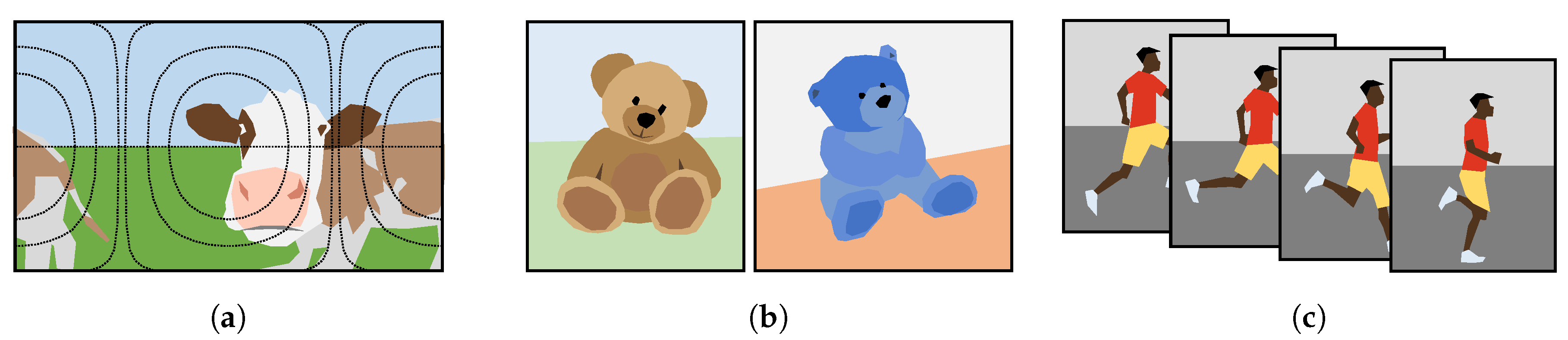
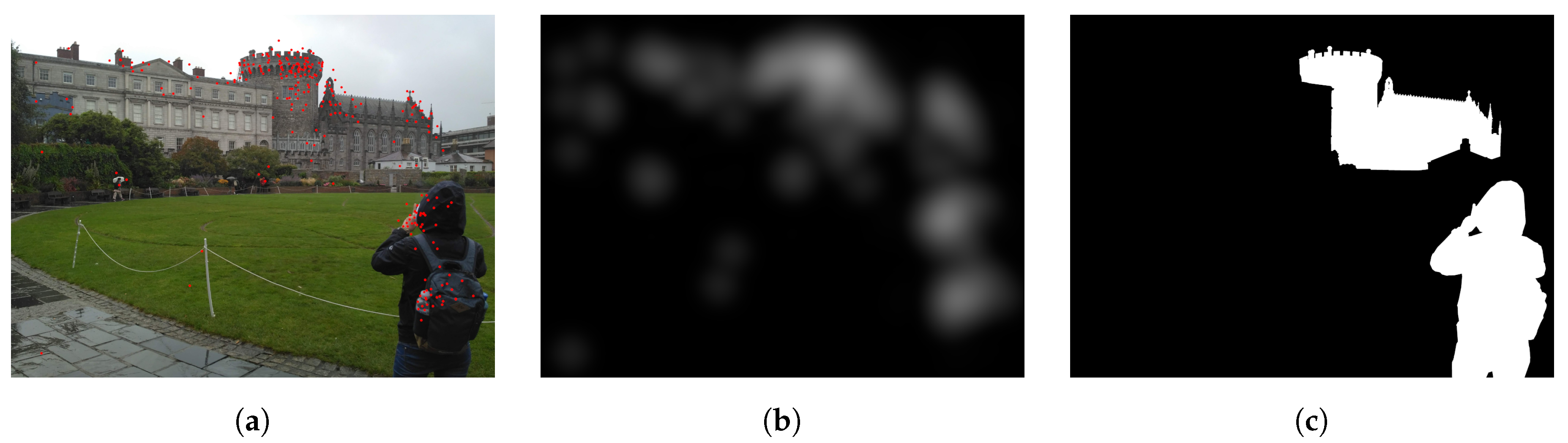
Table 1.
Characteristics of recent methods for visual saliency estimation in omnidirectional images. The “Target” column indicates the nature of the ground truth used to train or develop the methods, while “Output” describes what data they are explicitly able to generate (FM = Fixation maps, SP = Scanpaths).
| Method | 2D-to-ODI Adaptation | Custom Representation | Backbone CNN | Deep Learning | Hand- Crafted | Target | Output |
|---|---|---|---|---|---|---|---|
| Battisti 2019 [29] | (none) | ✓ | FM | FM | |||
| Sitzmann 2018 [33] | ✓ | (none) | ✓ | FM | FM | ||
| Monroy 2018 [61] | ✓ | VGG_CNN_M | ✓ | FM | FM | ||
| Ling 2018 [62] | (none) | ✓ | FM | FM | |||
| Lebreton 2018 [63] | ✓ | (none) | ✓ | FM | FM | ||
| Cheng 2018 [36] | ✓ | ResNet-50/VGG-16 | ✓ | FM | FM | ||
| Fang 2018 [64] | (none) | ✓ | FM | FM | |||
| De Abreu 2017 [34] | ✓ | (none) | ✓ | FM | FM, SP | ||
| Assens 2017 [35] | ✓ | VGG-16 | ✓ | FM, SP | FM, SP | ||
| Maugey 2017 [73] | ✓ | ✓ | (none) | ✓ | FM | FM |
Table 2.
Dataset/method matrix for visual saliency estimation in omnidirectional images.
| Dataset | Method | Battisti 2019 [29] | Sitzmann 2018 [33] | Monroy 2018 [61] | Ling 2018 [62] | Lebreton 2018 [63] | Cheng 2018 [36] | Fang 2018 [64] | De Abreu 2017 [34] | Assens 2017 [35] | Maugey 2017 [73] |
|---|---|---|---|---|---|---|---|---|---|---|---|
| Salient360! | (2017) [40] | ✓ | ✓ | ||||||||
| (2018) [41] | ✓ | ✓ | ✓ | ✓ | ✓ | ||||||
| SVR [33] | ✓ | ||||||||||
| Wild-360 [36] | ✓ | ||||||||||
| LAY [34] | ✓ | ||||||||||
| iSUN [77] | ✓ | ||||||||||
| MIT [78] | ✓ | ||||||||||
Table 3.
Datasets for visual saliency in omnidirectional images and related characteristics (FM = Fixation maps, SP = Scanpaths).
Table 3.
Datasets for visual saliency in omnidirectional images and related characteristics (FM = Fixation maps, SP = Scanpaths).
| Stimuli | Devices | ||||||
|---|---|---|---|---|---|---|---|
| Dataset | Video/Image | CGI/Real | Resolution (Pixels) | Duration (Seconds) | Conditions | Display | Eye Tracker |
| Salient360! [41] | Mixed | Mixed | 3000 × 1500 ÷ 18,332 × 9166 | 25 | Seated | Oculus DK2 | SMI |
| SVR [33] | Image | CGI | 8192 × 4096 | 30 | Seated, standing | Oculus DK2, PC screen | Pupil-labs, Tobii EyeX |
| Wild-360 [36] | Video | Real | 1920 × 960 | ∼20 (length) | N/A | PC screen | (none) |
| LAY [34] | Image | Real | 4096 × 2048 | 10, 20 | N/A | Oculus DK2 | (none) |
| Cardinalities | Responses | ||||||
| Dataset | Input Data | Users | Acquisitions | FM/SP | Head/Eyes | Project Page | |
| Salient360! [41] | 85 images/19 videos | 63 | ≤32 maps/paths per stimulus | FM, SP | Head, eyes | [79] | |
| SVR [33] | 22 images | 169 | 1980 maps/paths | FM, SP | Head, eyes | [80] | |
| Wild-360 [36] | 85 videos (29 ann.) | 30 | 12,926 maps | FM | (manual) | [81] | |
| LAY [34] | 21 images | 32 | 704 paths | SP | Head | [82] | |
Table 4.
Quantitative comparison of selected methods for saliency estimation in omnidirectional images, on the Salient360! challenge dataset. Best results are highlighted in boldface.
Table 4.
Quantitative comparison of selected methods for saliency estimation in omnidirectional images, on the Salient360! challenge dataset. Best results are highlighted in boldface.
| Method | ||||
|---|---|---|---|---|
| Monroy 2018 [61] | 0.536 | 0.487 | 0.757 | 0.702 |
| Ling 2018 [62] | 0.550 | 0.477 | 0.939 | 0.736 |
| Lebreton 2018 [63] | 0.527 | 0.698 | 0.851 | 0.714 |
| Fang 2018 [64] | 0.538 | 0.508 | 0.910 | 0.736 |
Table 5.
Characteristics of the analyzed methods for co-saliency estimation. The “Target” column indicates the nature of the ground truth used to train or develop the methods, while “Output” describes what data they are explicitly able to generate (OR = Object Regions, SM = Sharp saliency Maps, BM = Binary Masks).
| Method | Early Fusion | Late Fusion | Backbone CNN | Deep Learning | Deep Features | Hand- Crafted | Target | Output |
|---|---|---|---|---|---|---|---|---|
| Cong 2019-II [93] | ✓ | ✓ | (none) | ✓ | OR | SM | ||
| Zhang 2019 [67] | ✓ | FCN (VGG-16) | ✓ | OR | SM | |||
| Jerripothula 2018 [92] | ✓ | (none) | ✓ | OR | SM, BM | |||
| Hsu 2018 [94] | ✓ | ResNet-50 + FCN (VGG-16) | ✓ | OR | SM | |||
| Tsai 2018 [68] | ✓ | ✓ | CNN-S | ✓ | ✓ | OR | SM, BM | |
| Jeong 2018 [69] | ✓ | ✓ | DeepLab (VGG-16) | ✓ | OR | SM, BM | ||
| Zheng 2018 [95] | ✓ | FCN-32s (VGG-16) | ✓ | OR | SM | |||
| Cong 2018 [96] | ✓ | ✓ | VGG-16 | ✓ | ✓ | OR | SM | |
| Wang 2017-I [37] | ✓ | ✓ | (none) | ✓ | OR | SM, BM | ||
| Wei 2017 [70] | ✓ | FCN (VGG-16) | ✓ | OR | SM | |||
| Yao 2017 [89] | ✓ | (none) | ✓ | ✓ | OR | SM |
Table 6.
Dataset/method matrix for co-saliency estimation. The number in parentheses indicates the version of the MSRC dataset identified by the number of image groups.
Table 6.
Dataset/method matrix for co-saliency estimation. The number in parentheses indicates the version of the MSRC dataset identified by the number of image groups.
| Dataset | Method | Cong 2019-II [93] | Zhang 2019 [67] | Jerripothula 2018 [92] | Hsu 2018 [94] | Tsai 2018 [68] | Jeong 2018 [69] | Zheng 2018 [95] | Cong 2018 [96] | Wang 2017-I [37] | Wei 2017 [70] | Yao 2017 [89] |
|---|---|---|---|---|---|---|---|---|---|---|---|---|
| RGBD Coseg183 [30] | ✓ | ✓ | ||||||||||
| RGBD Cosal150 [96] | ✓ | ✓ | ||||||||||
| iCoseg [98] | ✓ | ✓ | ✓ | ✓ | ✓ | ✓ | ✓ | ✓ | ||||
| MSRC [86] | ✓(8) | ✓(14) | ✓(7) | ✓(14) | ✓(8) | ✓(7) | ✓(23) | ✓(7) | ||||
| Cosal2015 [87] | ✓ | ✓ | ✓ | ✓ | ✓ | |||||||
| Coseg-Rep [88] | ✓ | |||||||||||
| Internet Images [102] | ✓ | |||||||||||
| Image-Pair [103] | ✓ | |||||||||||
| Safari [104] | ✓ | |||||||||||
| Vicosegment [37] | ✓ | |||||||||||
Table 7.
Selected datasets for co-saliency estimation with corresponding characteristics (OR = Object Regions).
Table 7.
Selected datasets for co-saliency estimation with corresponding characteristics (OR = Object Regions).
| Stimuli | Cardinalities | ||||||||
|---|---|---|---|---|---|---|---|---|---|
| Dataset | Video/ Image | CGI/ Real | Resolution (Pixels) | Same Subject | Groups | Images Per Group | Total Images | Responses | Project Page |
| RGBD Coseg183 [30] | Image | Real | 640 × 480 | Yes | 16 | 6 ÷ 18 | 183 | OR | [105] |
| RGBD Cosal150 [96] | Image | Mixed | 303 ÷ 1177 | Mixed | 21 | 2 ÷ 20 | 150 | OR | [106] |
| iCoseg [98] | Image | Real | 333 ÷ 500 | Mixed | 38 | 4 ÷ 41 | 643 | OR | [107] |
| MSRC [86] | Image | Real | 320 × 213 | No | 14 | 24 ÷ 32 | 418 | OR | [108] |
| Cosal2015 [87] | Image | Real | 93 ÷ 3008 | No | 50 | 26 ÷ 52 | 2015 | OR | [109] |
| Coseg-Rep [88] | Image | Real | 137 ÷ 1280 | No | 22+1 | 9 ÷ 49 (+116) | 572 | OR | [110] |
| Internet Images [102] | Image | Real | 107 ÷ 340 | No | 3 | 561 ÷ 1306 | 2746 | OR | [111] |
| Image-Pair [103] | Image | Real | 66 ÷ 500 | Mixed | 105 | 2 | 210 | OR | [112] |
| Safari [104] | Video | Real | 270 ÷ 640 | Yes | 9 | 20 ÷ 50 | 415 | OR | [113] |
| Vicosegment [37] | Video | Real | 216 ÷ 480 | Yes | 10+38 | 18 ÷ 40 | 743 | OR | [114] |
Table 8.
Quantitative comparison of selected methods for co-saliency estimation on the iCoseg dataset. Best results are highlighted in boldface.
Table 8.
Quantitative comparison of selected methods for co-saliency estimation on the iCoseg dataset. Best results are highlighted in boldface.
| Method | |||
|---|---|---|---|
| Zhang 2019 [67] | 0.855 | 0.906 | 0.974 |
| Hsu 2018 [94] | 0.850 | 0.911 | - |
| Tsai 2018 [68] | 0.820 | 0.878 | 0.968 |
| Jeong 2018 [69] | 0.823 | 0.896 | 0.979 |
| Zheng 2018 [95] | 0.873 * | 0.920 * | - |
| Yao 2017 [89] | 0.810 | 0.868 | - |
* Values inferred from graphs in the corresponding publication.
Table 9.
Methods for video saliency. The temporal window is indicated in relation to the underlying technique: OF (Optical Flow), LSTM (Long-Short Term Memory), CNN (Convolutional Neural Network), GRU (Gated Recurrent Unit). The “Target” column indicates the nature of the ground truth used to train or develop the methods, while “Output” describes what data they explicitly generate (OR = Object Regions, SM = Sharp Maps, BM = Binary Masks, FM = Fixation Maps).
| Method | Saliency Shift | Temporal Window | Optical Flow | Backbone CNN | Deep Learning | Hand- Crafted | Target | Output |
|---|---|---|---|---|---|---|---|---|
| Fan 2019 [49] | ✓ | ∞ (LSTM) | ResNet-50 | ✓ | OR | SM | ||
| Li 2019 [127] | 2 (OF) | ✓ | ResNet-34/101 | ✓ | OR | SM | ||
| Yan 2019 [128] | 4 (CNN) + ∞(GRU) | ✓ | ResNet-50 | ✓ | OR | SM, BM | ||
| Cong 2019-III [129] | 2 (OF) + ∞ (energy) | ✓ | (none) | ✓ | OR | SM | ||
| Hu 2018 [125] | 2 (OF) + ∞ (diffusion) | ✓ | (none) | ✓ | OR | SM, BM | ||
| Zhou 2018 [130] | 3 | ✓ | (none) | ✓ | OR | SM | ||
| Ullah 2018 [121] | 2 (OF) | ✓ | (none) | ✓ | OR | SM, BM | ||
| Wang 2017-II [126] | 5 (OF) | ✓ | (none) | ✓ | OR | SM, BM | ||
| Chen 2017 [131] | 4 ÷ 20 (diffusion) | ✓ | (none) | ✓ | OR | SM | ||
| Min 2019 [65] | 32 (CNN) | S3D (inception) | ✓ | FM | FM | |||
| Gorji 2018 [66] | ✓ | ∞ (LSTM) | VGG-16 | ✓ | FM | FM |
Table 10.
Dataset/method matrix for video saliency estimation. The number in parentheses identifies the version of the dataset through the corresponding cardinality of video sequences.
Table 10.
Dataset/method matrix for video saliency estimation. The number in parentheses identifies the version of the dataset through the corresponding cardinality of video sequences.
| Dataset | Method | Fan 2019 [49] | Li 2019 [127] | Yan 2019 [128] | Cong 2019-III [129] | Hu 2018 [125] | Zhou 2018 [130] | Ullah 2018 [121] | Wang 2017-II [126] | Chen 2017 [131] | Min 2019 [65] | Gorji 2018 [66] |
|---|---|---|---|---|---|---|---|---|---|---|---|---|
| DAVSOD [49] | ✓ | |||||||||||
| FBMS [122] | ✓(30) | ✓ | ✓(59) | ✓(59) | ✓(59) | ✓(26) | ||||||
| ViSal [139] | ✓ | ✓ | ✓ | |||||||||
| MCL [140] | ✓ | |||||||||||
| SegTrack | v1 [138] | ✓ | ✓ | ✓ | ||||||||
| v2 [123] | ✓(13) | ✓(14) | ✓(14) | ✓(14) | ✓(14) | ✓(10) | ||||||
| UVSD [141] | ✓ | |||||||||||
| VOS [43] | ✓ | ✓ | ||||||||||
| DAVIS [124] | ✓ | ✓ | ✓ | ✓ | ✓ | |||||||
| I2R [142] | ✓ | |||||||||||
| Wallflower [143] | ✓ | |||||||||||
| MOViCS [117] | ✓ | |||||||||||
| DS [144] | ✓ | |||||||||||
| UCFSports [134,145] | ✓ | ✓ | ✓ | ✓ | ||||||||
| DHF1K [135] | ✓ | |||||||||||
| Hollywood-2 [134,146] | ✓ | ✓ | ||||||||||
| DIEM [147] | ✓ | |||||||||||
Table 11.
Selected datasets for video saliency estimation, with related features (SP = Scanpaths, FX = Fixations only, FM = Fixation maps, OR = Object Regions).
Table 11.
Selected datasets for video saliency estimation, with related features (SP = Scanpaths, FX = Fixations only, FM = Fixation maps, OR = Object Regions).
| Stimuli Characteristics | Devices | Users | ||||
|---|---|---|---|---|---|---|
| Dataset | Resolution (pixels) | FPS | Display | Eye Tracker | Users (Fixations) | Users (Objects) |
| DAVSOD [49] | 640 × 360 | 30 | N/A | SMI RED 250 | 17 (1/video) | 20 |
| FBMS [122] | 288 ÷ 960 | 30 | N/A | (none) | (none) | N/A |
| SegTrack v2 [123] | <640 × 360 | N/A | N/A | (none) | (none) | N/A |
| VOS [43] | 800 × 448 | 30 | 1680 × 1050 | SMI RED 500 | 23 | 4 |
| DAVIS [124] | 1920 × 1080 | 24 | N/A | (none) | (none) | N/A |
| UCFSports [134] | <720 × 480 | 10 | 22" 1280 × 1024 | SMI iView X HiSpeed 1250 | 16 | (none) |
| DHF1K [135] | 640 × 360 | 30 | 19 1440 × 900 | SMI RED 250 | 17 (1/video) | (none) |
| Cardinalities | Responses | |||||
| Dataset | Total Videos | Total Frames | Frames Per Video | SP/FX/FM/OR | Project Page | |
| DAVSOD [49] | 187 | 23,938 | ∼128 | FX, FM, OR | [148] | |
| FBMS [122] | 59 | 13,860 (720 annotated) | ∼235 (∼12 annotated) | OR | [149] | |
| SegTrack v2 [123] | 14 | 1066 | ∼76 | OR | [150] | |
| VOS [43] | 200 | 114,421 (7467 annotated) | ∼722 (∼37 annotated) | OR | [151] | |
| DAVIS [124] | 50 | 3455 | ∼69 | OR | [152] | |
| UCFSports [134] | 150 | 9578 | ∼64 | SP | [153] | |
| DHF1K [135] | 1000 | 582,605 | ∼583 | FX, FM | [154] | |
Table 12.
Quantitative comparison of selected methods for video saliency estimation on the SegTrack v2 and DAVIS datasets. Best results are highlighted in boldface.
Table 12.
Quantitative comparison of selected methods for video saliency estimation on the SegTrack v2 and DAVIS datasets. Best results are highlighted in boldface.
| Method | SegTrack v2 | DAVIS | ||
|---|---|---|---|---|
| ↑ | MAE↓ | ↑ | MAE↓ | |
| Fan 2019 [49] | 0.801 | 0.0230 | - | - |
| Li 2019 [127] | - | - | 0.902 | 0.0220 |
| Yan 2019 [128] | - | - | 0.859 | - |
| Cong 2019-III [129] | - | - | 0.765 | 0.0588 |
| Zhou 2018 [130] | 0.899 * | 0.0807 * | 0.747 * | 0.0636 * |
| Wang 2017-II [126] | 0.890 * | 0.0489 * | - | - |
| Chen 2017 [131] | 0.810 * | - | - | - |
* Values inferred from graphs in the corresponding publication.
© 2020 by the author. Licensee MDPI, Basel, Switzerland. This article is an open access article distributed under the terms and conditions of the Creative Commons Attribution (CC BY) license (http://creativecommons.org/licenses/by/4.0/).
Share and Cite
MDPI and ACS Style
Buzzelli, M. Recent Advances in Saliency Estimation for Omnidirectional Images, Image Groups, and Video Sequences. Appl. Sci. 2020, 10, 5143. https://doi.org/10.3390/app10155143
AMA Style
Buzzelli M. Recent Advances in Saliency Estimation for Omnidirectional Images, Image Groups, and Video Sequences. Applied Sciences. 2020; 10(15):5143. https://doi.org/10.3390/app10155143
Chicago/Turabian StyleBuzzelli, Marco. 2020. "Recent Advances in Saliency Estimation for Omnidirectional Images, Image Groups, and Video Sequences" Applied Sciences 10, no. 15: 5143. https://doi.org/10.3390/app10155143
Note that from the first issue of 2016, this journal uses article numbers instead of page numbers. See further details here.