Modeling Future Streamflow for Adaptive Water Allocation under Climate Change for the Tanjung Karang Rice Irrigation Scheme Malaysia

Abstract

Spatial and temporal climatic variability influence on the productivity of agricultural watershed and irrigation systems. In a large irrigation system, the quantification and regulation of the flow at different locations of the channel is quite difficult manually, leading to a poor delivery of supply and demand. Water shortage is a crucial issue due to mismatch between available water and demand at intake point of Tanjung-Karang Irrigation Scheme. This study assessed the potential impacts of climate change on basin outflow for 2010–2039, 2040–2069, and 2070–2099 to the baseline period (1976–2005) and used it as input hydrograph to simulate river discharge. A Hydrologic Engineering Corps Hydrologic Modeling System (HEC-HMS) model driven by projections from ten global climate models (GCMs) with three scenarios (Representative Concentration Pathways (RCPs) 4.5, 6.0, and 8.5) used to simulate the outflow and the Hydrologic Engineering Centers River Analysis System (HEC-RAS) model applied for hydraulic modeling. The projected seasonal streamflow showed a decreasing trend for future periods. The average available irrigation supply for historical period is 15.97 m³/s, which would decrease by 12%, 18%, and 21% under RCPs 4.5, 6.0, and 8.5, respectively. Projected irrigation supply showed oversupply and undersupply to the required supply during the growing season. Simulated discharge could therefore be incorporated into cropping practices to boost the sustainable distribution of water under the new realities of climate change in the future.

1. Introduction

Irrigation system is an essential component for optimal agricultural production. The design, construction, operation, and maintenance of hydraulic projects in irrigation schemes require adequate information with the exact magnitude and the actual time of occurrence of all streamflow events at present and in the future. The irrigation sector utilizes the highest portion of human accessible water from rivers, lakes and aquifers with about 2500 km³ year⁻¹ globally, which represents about 70% of total human water use [1]. The effective use of available fluctuating river inflows for irrigation is one of the crucial strategies for proper planning and management of a river-fed irrigation system [2]. Water availability and its coherent quantification in the respective river basins and also on a global scale have been a great challenge [3,4].

Variations in temperature and rainfall seem to be the most widely reported problems plaguing predicted climate change in the next century [5]. However, these variations differ significantly across the place in the world. For example, a catchment located in a temperate climate could respond differently to the impact of climate change compared to a catchment situated in a mountain climate [6]. Climate change has a significant effect in altering rainfall patterns in humid tropics [7]. Therefore, the change in rainfall patterns is more significant than in the climate change temperatures in a tropical region like Malaysia [8]. Although Malaysia is blessed with abundant water resources, many regions suffer water shortages because of spatial and temporal variability of precipitation, which resulted in incremental demand for water resources [2]. Consequently, rivalry for actual water supplies is now more crucial. Most of the country’s rice farming systems rely mainly on river streamflow. However, due to insufficient flow in the rivers, particularly during the dry season (January to June), some rice schemes incorporate reservoir to river headwork, to meet water requirements for irrigation. Although water storage is a good option in the global water cycle and climate change [9], the design and operation of these storage facilities should be linked with the projected available water resources for adaptive water allocation.

Several research works were carried out to understand the variability of streamflows due to climate change [10,11,12,13,14,15] with mixed results in the streamflow variability, depending on the region and season. For instance, a decrease in annual streamflow was observed [5,16]. A similar trend was obtained when the hydrologic impacts of climate change were assessed on the runoff trend in Klang Watershed, Malaysia [17]. The results predicted annual mean streamflow for future periods to decrease, except the period 2080s. The maximum absolute increase in the mean peak runoff was projected in May and October for the 2080s due to high volume of precipitation. Moreover, a decrease in future streamflow was reported during the dry season period [18]. However, an overall increase of streamflows was found in [19].

In a large irrigation scheme, it is quite hard to manually quantify and regulate flow at different sections of a channel, resulting in inadequate delivery between supply and demand. In [20], the drawbacks with the application of conventional methods in irrigation has been highlighted. The Bernam River Basin is the primary source of irrigation supply for the Tanjung Karang Rice Irrigation Scheme Malaysia. The diversion of water for irrigation is from the Basin at the Bernam River Headworks (BRH) and reaches the scheme at Tengi River Headworks (TRH) over 24.5 km through a feeder canal of 14.5 km length. The hydrological and hydraulic processes of this river basin under climate change are paramount to the planning and management of the irrigation scheme’s potential water requirements. Water shortage is an annual issue for the scheme. An imbalance between water supply from the upstream and the water demand at the intake of the scheme is often experienced [21]. This consequently results in either water shortage at high demand or water wastage at the period of low demand.

Models are very useful tools in assessing water resources in irrigation systems [22]. Various computerize hydraulic models were developed and applied in different irrigation schemes to address related problems. For example, DUFLOW, MODIS, and CARIMA models were respectively evaluated by [23,24,25]. MIKE 11 and MIKE SHE models were applied in an irrigation project [26]. The Hydrologic Engineering Centers River Analysis System (HEC-RAS) is a hydraulic modeling software developed by the U.S. Army Corps of Engineer´s Hydrologic Engineering Center. It has the advantage of generating river geometry using spatial data with the Geographic information system (GIS) component of the model (HEC-GeoRAS), which is very helpful in canals with data scarcity. However, research on the hydraulic modeling of an irrigation system using the HEC-RAS model is very limited [27] with almost no study on water allocation for an irrigation scheme. The increasing water demand pressure continues to be concerned with the planning of paddy irrigation, based on the predicted multi-models global climate model (GCM) climate data series. Irrigation managers need an interactive tool that helps quick decisions on water management to reduce water and food safety risk. This study therefore implemented HEC-RAS and Hydrologic Engineering Corps Hydrologic Modeling System (HEC-HMS) to model the fluctuating river discharge in order to allocate adaptive water to a Malaysian irrigation system in the new realities of climate change.

2. Materials and Methods

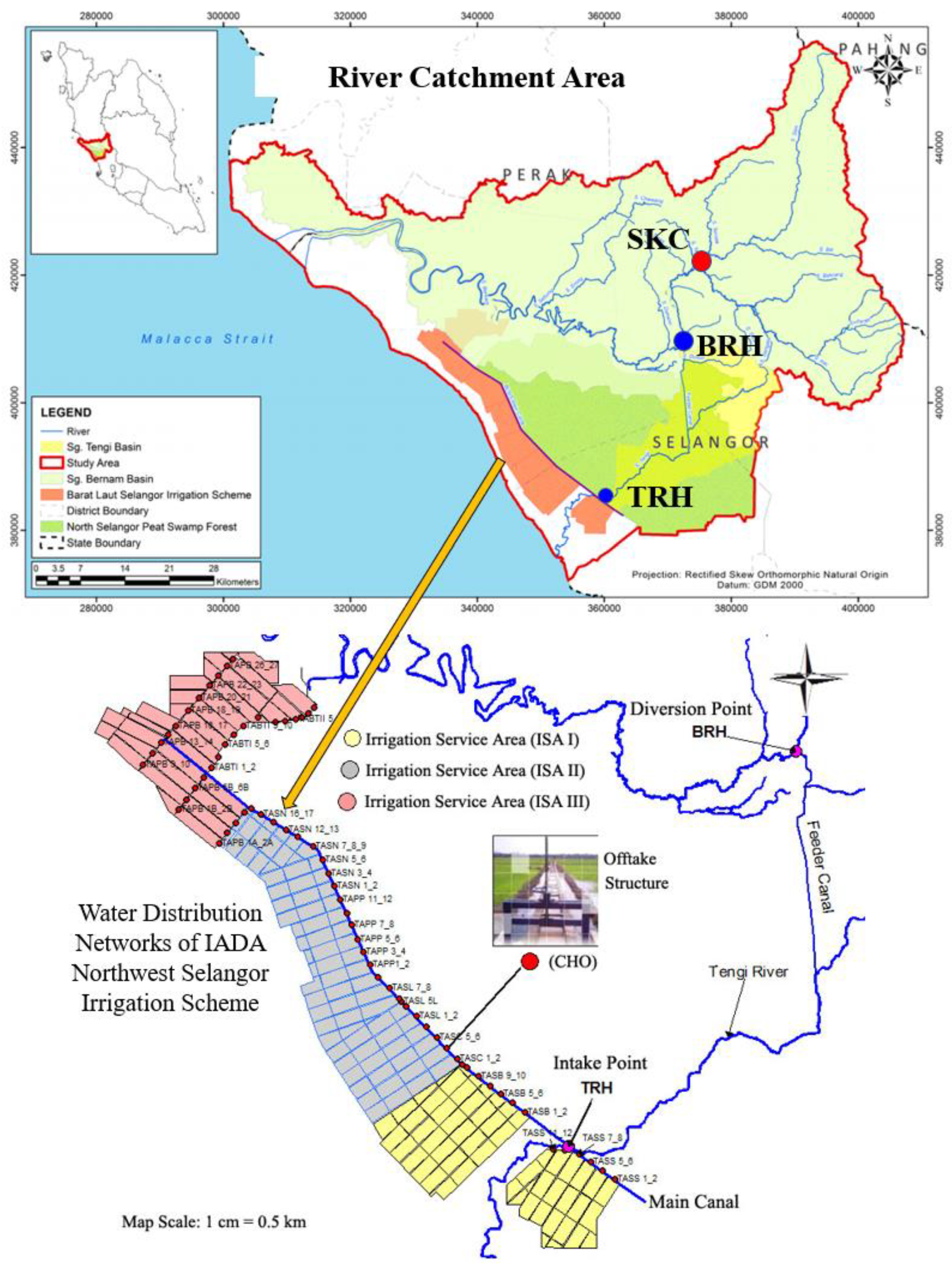
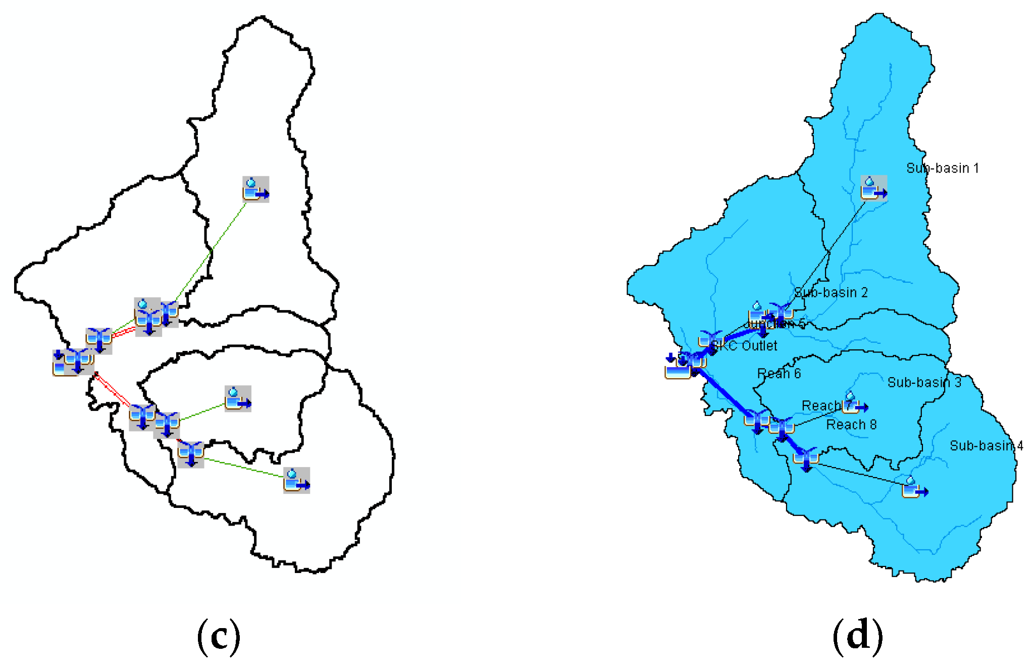
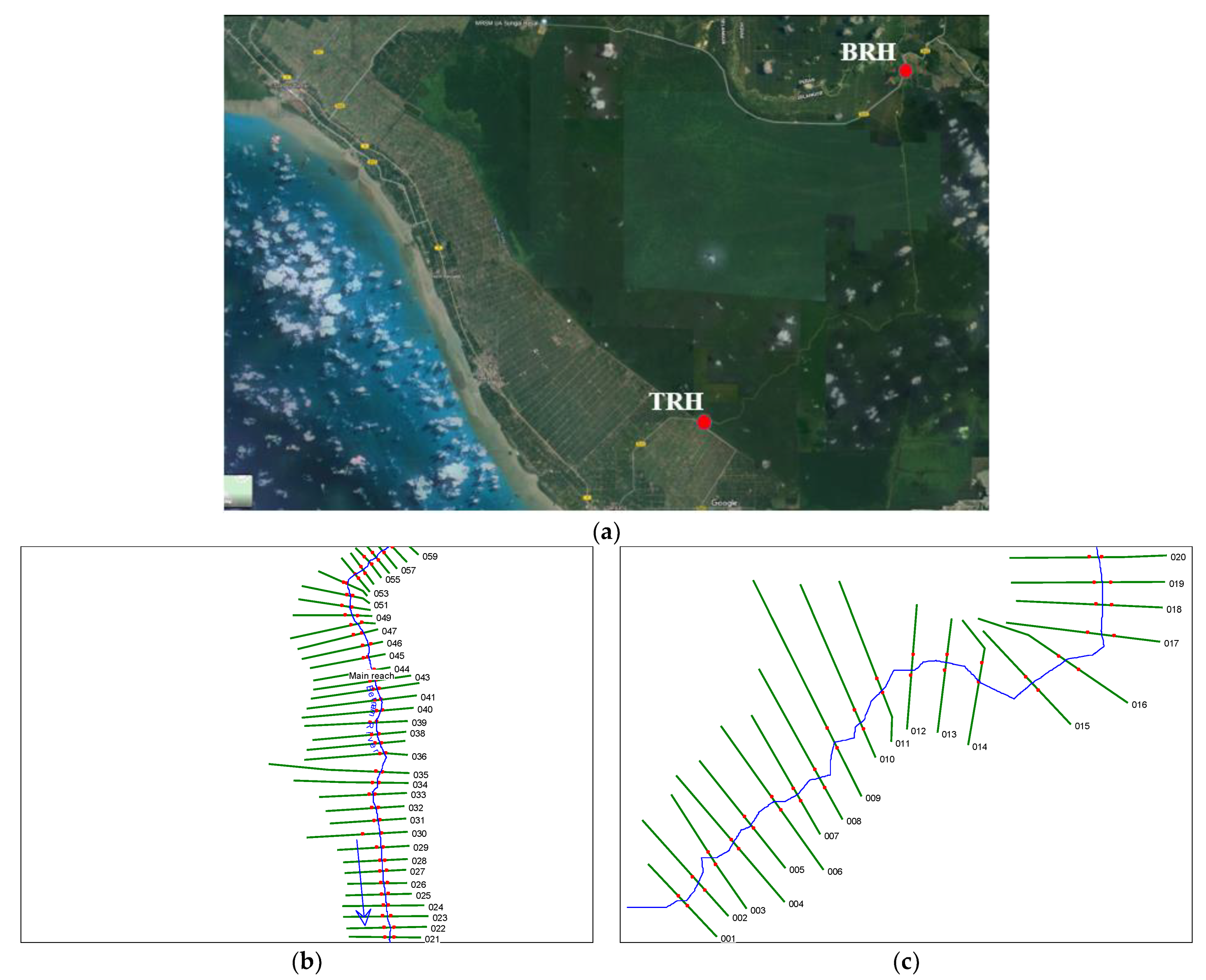
2.1. Study Area

Tanjung Karang Rice Irrigation Scheme (TAKRIS) is located at about latitude 3°25′ to 3°45′ N and longitude 100°58′ to 101°15′ E within the State of Selangor of Peninsular Malaysia on a coastal plain in Kuala Selangor District (Figure 1). The scheme is the fourth largest rice producing schemes in the country with a net command area of about 18,848 ha. Paddy is the predominant crop in the area. The runoff of the Upper Bernam river basin is the main source of irrigation water for the scheme. The climate of the area is a humid equatorial with bimodal rainfall patterns mostly influenced by the southwest and northeast monsoons. The average annual rainfall in the region is about 2000 mm, and its distribution is mostly between the months of October–January and only to a limited extent over April–May. However, the distribution of rainfall is unpredictable between the months of January–August and consequently crops rely mostly on irrigation during that period for yield sustenance. The average monthly temperature is 28 °C, with a daily variability of 8 °C and a monthly average humidity of 77% [28]. To ensure adequate irrigation deliveries to fields and better water management practices, the rice cultivation in the area has been staggered into four Irrigation Service Areas (ISAs I, II, III, and IV) from January (ISA I) to June (ISA IV) during the dry season (

Table 1. Present crop calendar and distribution of irrigation supplies in Tanjung Karang Rice Irrigation Scheme.

Activities	Dry-Season				Wet-Season
	ISA_I	ISA_II	ISA_III	ISA_IV	ISA_I	ISA_II	ISA_III	ISA_IV
Pre-saturation	1-January	1-February	1-March	1-April	1-July	1-August	1-September	1-October
Sowing starts	15-January	15-February	15-March	15-April	15-July	15-August	15-September	15-October
Normal irrigation	1-February	1-March	1-April	1-May	1-August	1-September	1-October	1-November
Irrigation ends	10-April	10-May	10-June	10-July	10-October	10-November	10-December	10-January

). The process is replicated for the wet season from July (ISA I) until October (ISA IV) before the heavy rains start.

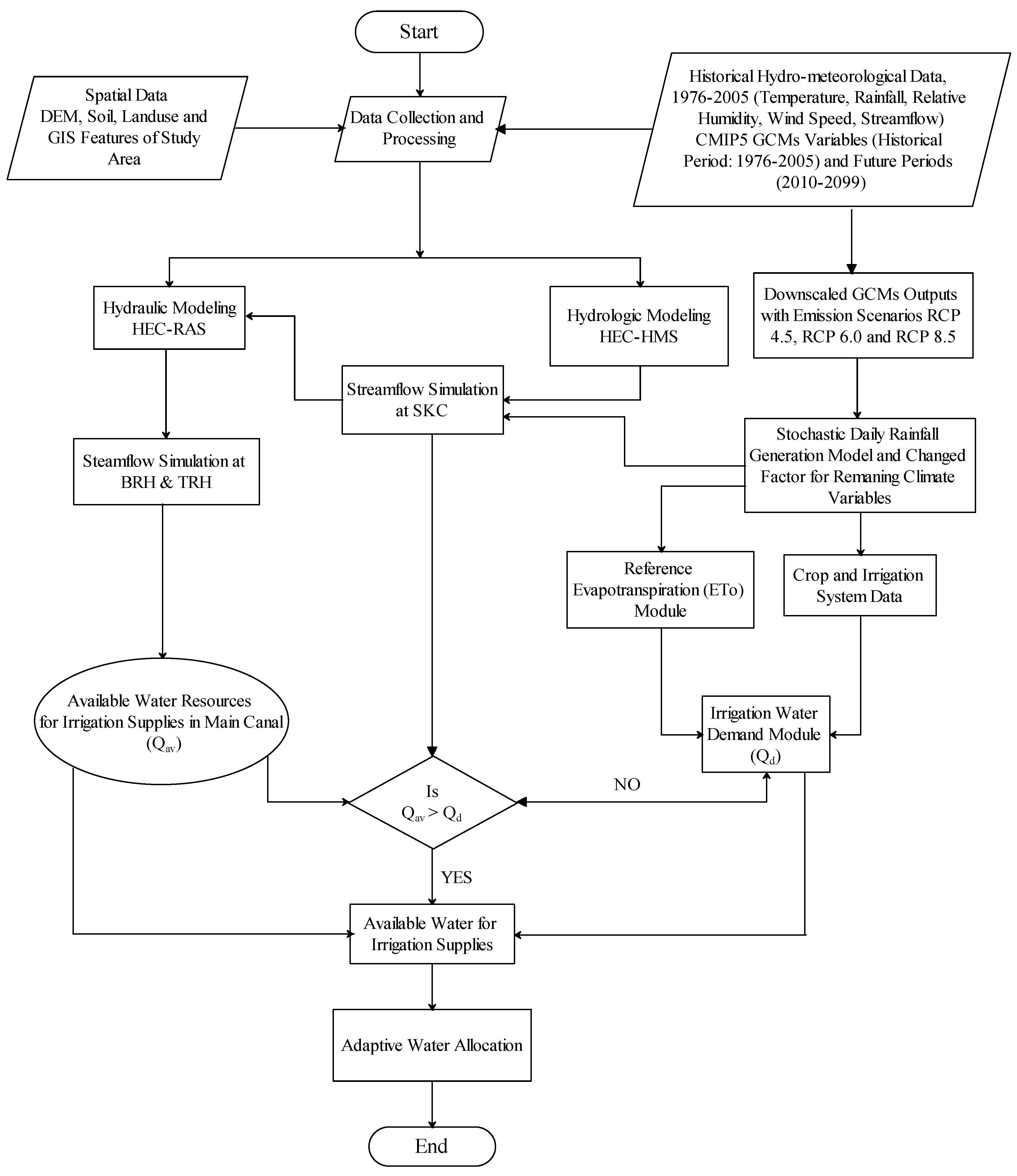
2.2. Methodological Approach

The study involves three major stages for the adoptive water allocation under climate change, namely: (1) extraction and downscaling of daily climate variables to a local station, (2) simulation of climate change impacts on hydrological processes in Upper Bernam River Basin (UBRB), and (3) assessment of available water resources in the main water conveyance system for adaptive water allocation with the need for scheme water demand under future climate change.

Climate variables for baseline (1976–2005) and future (2010–2099) periods were extracted from ten global climate models (GCMs) under three Representative Concentration Pathways (RCPs) scenarios (RCP 4.5, RCP 6.0, and RCP 8.5). The data was downscaled using a developed Climate-smart Decision Support System (CSDSS). The HEC-HMS hydrological model simulated climate change impacts on hydrological processes in UBRB and the HEC-RAS hydraulic model used to compute available discharges for the main water conveyance system from the Bernam River Headworks (BRH) to TRH and at the key points in the main canal. The spatial data required by the models were processed using GIS extension of the sofware in ArcGIS. The available water resources for adaptive water allocation in the main water conveyance system was assessed with the need for irrigation water demand under future climate change. The systematic approach for the study is depicted in Figure 2.

2.3. Downscaling of GCMs Outputs

Adoption of multi-models is essential and recommended for impact studies and adaptation strategies [30,31], because single GCM does not actually provide useful information in assessing the climate change impacts. Therefore, ten global climate projections were acquired from Program for Climate Model Diagnosis and Inter-comparison (PCMDI). A baseline period (1976–2005) was adopted and three future periods of 30-year time segments were defined as the 2020s (2010–2039), 2050s (2040–2069), and 2080s (2070–2099) under three RCP scenarios (RCP 4.5, RCP 6.0, and RCP 8.5). The spatial resolution from the output of GCMs cannot provide a good climate change scenario for a specific watershed, since GCMs run on a broad spatial scale. Hence, downscaling is needed to represent the impact of climate change on a catchment area. A developed CSDSS for downscaling hydro-meteorological variables [32], was adopted to downscale the extracted GCMs outputs. The CSDSS was built in Matrix Laboratory (MATLAB) environment using “Delta change factor” statistical downscaling method. The method has been widely applied in hydrological modeling because it allows speed of application, direct scaling of the scenarios with respect to changes suggested by the GCMs and also multi-models could be used with result from various GCM scenarios [33,34]. In the “Delta change factor” method, the mean values of GCM simulated baseline and future climates were estimated as [16]:

$$\overline{GC{M}_b}={{\displaystyle \sum }}_{i=1}^{Nb}GC{M}_{bi}/N_b,$$

(1)

$$\overline{GC{M}_f}={{\displaystyle \sum }}_{i=1}^{Nf}GC{M}_{fi}/N_f,$$

(2)

where, $\overline{GC{M}_b}$ and $\overline{GC{M}_f}$, GCM_b, and GCM_f are the mean values and values from GCM baseline and GCM future climate scenario, respectively. N_b and N_f are the total number of values in the downscaling for baseline and future periods, respectively.

The monthly additive (CF_add) and multiplicative Change Factor (CF_mul) changes between the baseline period and future period in the equivalent climate variable of interest were calculated for the GCM grid box using equations 3 and 4. Relative change factors were used in the case of rainfall (∆P), derived from the ratio of projected-to-baseline averages, while absolute change factors were used for temperature, relative humidity, solar radiation and wind speed (∆T), by subtracting the GCMs averages representing baseline from the future.

$$C{F}_{Rain}=\left(\raisebox{1ex}{${\overline{P}}_{GCM,fut,m}$}\!\left/ \!\raisebox{-1ex}{${\overline{P}}_{GCM,base,m}$}\right.\right),$$

(3)

$$C{F}_{Temp}=\left({\overline{T}}_{GCM,fut,m}-{\overline{T}}_{GCM,base,m}\right),$$

(4)

Finally, local scaled future climate values were obtained by applying the Change Factors using Equations (5) and (6). This involves superimposing the change factors suggested by the GCM-scenario combinations to the daily baseline time series to give perturbed climate series.

$$P_{adj,fut,d}=P_{obs,d}\times C{F}_{Rain},$$

(5)

$$T_{fut,d}=T_{obs,d}+C{F}_{Temp},$$

(6)

where, P and T are the rainfall and climatic variables, respectively, the subscript; adj,fut,d denotes the downscaled future daily variable; obs,d denotes daily observations; CF denotes calculated additive and multiplicative change factors for rainfall and climatic variables; GCM,fut,m and GCM,base,m are the average monthly values of GCM output and baseline periods, respectively.

A simulation dialog window appears after clicking on a specific command button from the CSDSS main dialog window, to generate daily hydro-meteorological variable(s) as shown in Figure 3. The program was calibrated and validated using the observed and simulated monthly average values for the baseline period. The outputs can be viewed from the “Analysis and Statistics” button as tables and graphs.

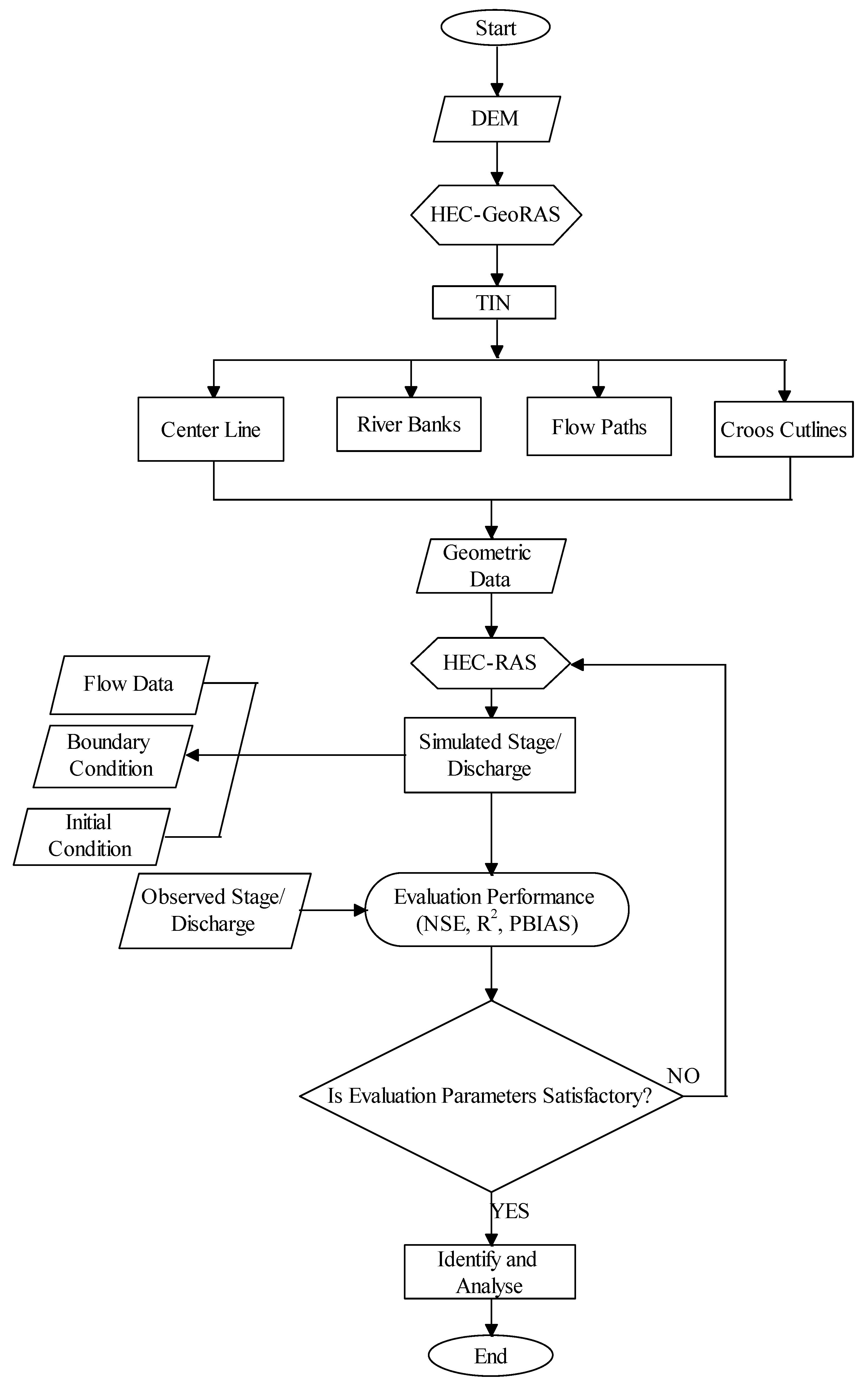
2.4. Modeling Future Impacts of Climate Change on Hydrological Processes

A recent version of hydrologic modeling software developed by the U.S. Army Corps of Engineers Hydrologic Engineering Centre (HEC-HMS 4.2.1) was used for simulating precipitation-runoff processes of upper Bernam watershed systems. The model requires two types of data: the spatial and climatic data. The spatial data used include digital elevation model (DEM), downloaded from Geographic information software program (DIVA-GIS) website, maps of soil and land use of the area obtained from Department of Agriculture (DOA) Malaysia while daily archives of the hydro-climatic data from 1976–2006, obtained from the Water Resources and Hydrology Division, Department of Irrigation and Drainage (DID) Malaysia, which include rainfall, temperature (minimum and maximum), relative humidity, wind speed and solar radiation were used. The HEC-HMS model components include basin models, meteorological models, control specifications, and input data. The components were used to simulate the hydrologic response in the Bernam watershed. The spatial data collected was used to set up the basin model using HEC-GeoHMS to calculate parameters, such as sub-basin areas, times of concentration, lag time, and reach lengths based on the DEM geospatial information.

The hydrological elements consist of sub-basin, reach, junction, sink (outlet), and diversion within the watershed as shown in Figure 4. Land use map of the area was processed into eleven classes. These include Aquaculture, Forest, Marshland, Oil palm, Paddy, Pasture, Rubber, Secondary forest, Swamp forest, Urban, and Waterbody. The size of the land use classes of Bernam catchment ranges from 0.2 to about 41% with the largest area dominated by forest followed by Oil Palm then Rubber. Moreover, the forest area contributed more for the impervious surfaces in the watershed followed by Oil Palm area then area covered by Rubber. Impervious area is a portion of the watershed for which all contributing precipitation runs off, with no infiltration, evaporation or other volume losses. This is expected considering the nature of the land use within the watershed, which is majorly forest and oil palm. Similarly, the soil was classified into two major hydrologic soil groups, namely groups B and C. About 84% and 16% of soil groups B and C, respectively dominate the soil in Bernam watershed. The group B soils typically have from 10%–20% clay and 50%–90% sand, and have loamy sand or sandy loam textures, with moderately low runoff potential when thoroughly wet. Whilst group C soils typically have from 20%–40% clay and less than 50% sand and have loam, silt loam, sandy clay loam, clay loam, and silty clay loam textures with moderately high runoff potential when thoroughly wet. This means less runoff amount is averagely expected in the area. The sizes of the merged sub-basins range between 160.49 km² and 370.32 km². Land use and soil grids were processed to obtain percentage of impervious area, maximum deficit, initial deficit and constant rate of each sub-basin as presented in

Table 2. Characteristics of delineated sub-basins of Bernam watershed.

Sub-Basin No.	Area (km2)	Initial Deficit (mm)	Maximum Deficit (mm)	Constant Rate (mm/h)	Impervious Surface (%)
1	325.38	50.46	52.50	48.45	2.51
2	370.32	47.64	51.65	49.50	4.28
3	160.49	50.55	51.50	50.50	5.10
4	261.10	49.43	50.36	48.44	3.83

.

The sub-basin element in HEC-HMS model conceptually represents interactions of infiltration, surface runoff, and subsurface processes. Priestly-Taylor method was used to compute the potential evapotranspiration, $ET$ (mm/day) as mostly used in continuous simulation using HEC-HMS [19]. The model is expressed as [35]:

$$ET=\frac{\alpha }{\lambda }\frac{\Delta }{\Delta +\gamma }\left(R_n-G\right),$$

(7)

where, α = 1.26, λ is latent heat of evaporation (MJ/kg), R_n is net radiation at crop surface (MJ m⁻² day⁻¹), G is soil heat flux density (MJ m⁻² day⁻¹), Δ is slope vapor pressure curve (kPa °C⁻¹), and γ is Psychrometric constant (kPa °C⁻¹).

The Deficit and Constant Loss (DCL) method was used to compute the runoff-volume (loss). It uses one layer to account for continuous changes in moisture and requires only four parameters namely initial deficit, maximum deficit, constant rate, and percentage of impervious area. The method is simple, requires lesser-input parameters and can be applied for event-based and long-term simulations [36] and applied by many studies [19,37,38,39]. The DCL parameters were obtained from the land use and soil grids of the area using HEC-GeoHMS, a GIS extension of HEC-HMS. The DCL method was combined with simple canopy and surface methods. The canopy method accounts for precipitation intercepted by plants from one storm to another, which subsequently evaporates and the water extracted by the plants through the process of transpiration. The surface method on the other hand accounts for the maximum amount of water that held on the soil before surface runoff begins. Soil Conservation Service Unit hydrograph (SCS-UH) method was used for the transformation of precipitation excess into point runoff. The method is applicable for long-term simulation [19]. In this method, unit hydrograph (UH) discharge, U_t is given as a ratio to the UH peak discharge, U_p, for any time t, a fraction of T_p, the time to UH peak [36]:

$$U_p=C\frac{A}{T_p},$$

(8)

$$T_p=\frac{\Delta t}{2}+t_{lag},$$

(9)

where, A is the watershed area, C is the conversion constant (2.08), $\Delta t$ is duration of excess precipitation, and $t_{lag}$ is the basin lag. The input parameter for this method is the basin lag, which is 0.6 times the time of concentration $t_c$ of the flow. The $t_c$ was obtained using HEC-GeoHMS and adjusted through calibration process.

The baseflow in each sub-basin was modeled using constant monthly-varying method. In this method, the program represents baseflow as a constant flow but may vary monthly. The monthly flows were approximated from the long-term series of monthly-observed flow data and were added to the direct runoff, computed from rainfall for each time step of the simulation. The channel flow was computed using Muskingum routing method as widely adopted by many studies [19,37,38,39] because of its wider considerations to most conditions of watershed and it accounts for streamflow attenuation. The method consists of two parameters; the travel time through the reach, K and a weighing factor, X. The parameters K and X were estimated using the channel geometry. The travel time, K (h) was computed using equation 10 [40]:

$$K=\frac{L}{3600V_w},$$

(10)

where L is the reach length (m) and V_w is the flood wave velocity (m/s).

Historical discharge records were used for evaluating the performance of the HEC-HMS model. Manual and automatic calibration techniques were applied to optimize model parameters. Discharge data for 18 years (1981–1998) was used for model calibration and 8 years (1999–2006) for validation with 5 years of warm up period in each. To project the future streamflow regime in the Bernam basin, the downscaled GCMs outputs for the baseline (1976–2005) and future (2010–2099) periods, which include rainfall, temperature, solar radiation, relative humidity, and wind speed, were used as input to the validated HEC-HMS model. Flow simulation was performed for each RCP scenario for 30-year time segments centered on the three future periods. For long-term analysis, data was prepared in accordance with the ‘period change’ approach by defining future periods as: (i) 2020s (2010–2039), (ii) 2050s (2040–2069), and (iii) 2080s (2070–2099), to analyze change from a defined baseline period.

2.5. Computation of Available Discharges for Irrigation Supply

HEC-RAS model, which is a computer program that models the hydraulics of water flow through natural rivers and other channels, was adopted in the present study. The HEC-RAS 5.0 with Geospatial Hydrologic Modeling extension (Arc-Hydro and HEC-GeoRAS) was used. The model is capable of performing one-dimensional (1-D) steady and unsteady-flow simulations. The unsteady, gradually varied flow simulation model is dependent on finite difference solutions of the Saint–Venant equations as presented in Equations (1) and (2) [41]:

$$\frac{\partial A}{\partial t}+\frac{\partial Q}{\partial x}=0,$$

(11)

$$\frac{\partial Q}{\partial t}+\frac{\partial \left(\frac{Q^2}{A}\right)}{\partial x}+gA\frac{\partial H}{\partial x}+gA\left(S_o-S_f\right)=0,$$

(12)

where: A—cross-sectional area normal to the flow; Q—discharge; g—acceleration due to gravity; H—elevation of the water surface above a specified datum, also called stage; S_o—bed slope; S_f—energy slope; t—temporal coordinate, and x—longitudinal coordinate.

The data needed to perform the computations are categorized into two; geometric data and flow data. The basic geometric data in HEC-RAS comprise of establishment of the river system connectivity (river system schematic); cross section data; reach lengths; energy loss coefficients (friction losses, contraction and expansion losses); stream junction information; etc. Prior to using the HEC-RAS model, a DEM raster of the study area was downloaded from DIVA-GIS, converted to triangular irregular network (TIN) within Arc-GIS. The TIN was used to establish the river system connectivity; cross-section data, reach length, etc. using HEC-GeoRAS coupled with Arc-Hydro tool. After pre-processing stages using HEC-GeoRAS, the information that clarifies the shape, height and position and the overall cross section traits of channel were extracted and exported into the HEC-RAS model. Figure 5 summarized the HEC-RAS model setup for the study.

The most sensitive calibration parameter required by the HEC-RAS model is channel resistance—specifically Manning’s n. Its values can be extracted with the aid of land use map of the area using HEC-GeoRAS. However, due to insufficient land use data, covering all the river area, n values presented by another study [42] was used as a first estimate of the appropriate channel resistance and adjusted through calibration. The contraction coefficient was fixed to 0.1 and the coefficient of expansion was fixed to 0.3. The changes in cross sections is a common cause of energy losses within a reach (between two cross sections), which usually results in contraction or expansion of flow. The contraction or expansion coefficients used in the model were selected as reported by [41]. Unsteady flow data comprise of boundary conditions (external and internal) and initial conditions. The earlier simulated streamflow at the basin outlet by HEC-HMS model was used as input hydrograph to the HEC-RAS model for flow routing in the river. The downstream end of the river was modeled with the flow hydrograph at the intake of main canal (TRH). Moreover, the initial condition was established automatically by the software.

Because of irregular and limited flow data at the downstream side, located at the inlet of the main canal, reliable data for four years (from 2001 to 2004) was used for model evaluation. The model was calibrated by comparing between the simulated and observed values using the 2001–2003 daily discharge records of the river. Finally, the calibrated model was validated using the 2004 daily discharge records.

2.6. Statistical Evaluation of Models

The performance of the models was evaluated by comparing the observed discharge with the simulated data using the most commonly used statistical indices as:

(i)

Coefficient of Determination (R²) [43]

$${\mathrm{R}}^2={\left(\frac{{{\displaystyle \sum }}_{i=1}^n\left(P_i^{obs}-P_i^{mean}\right)\left(P_i^{sim}-P_i^{mean}\right)}{{\left[{{\displaystyle \sum }}_{i=1}^n{\left(P_i^{obs}-P_i^{mean}\right)}^2{{\displaystyle \sum }}_{i=1}^n{\left(P_i^{obs}-P_i^{sim}\right)}^2\right]}^{0.5}}\right)}^2,$$

(13)

(ii)

Nash–Sutcliffe Efficiency (NSE) [44]

$$\mathrm{NSE}=1-\frac{{\displaystyle \sum _{i=1}^n}{(Q{o}_i-Q{s}_i)}^2}{{\displaystyle \sum _{i=1}^n}{(Q{o}_i-\overline{Q}o)}^2},$$

(14)

(iii)

Percentage bias (PBIAS) [45]

$$\mathrm{PBIAS}=\frac{{{\displaystyle \sum }}_{i=1}^N\left(Q_{oi}-Q_{si}\right)}{{{\displaystyle \sum }}_{i=1}^N{Q}_{oi}}\times 100\%,$$

(15)

2.7. Water Demand Estimation

To compute the daily water demand in the paddy area, a water balance model for a paddy field was employed, which is given by [28]:

$$S{W}_{t+1}=S{W}_t+I{R}_t+E{R}_t-E{T}_t-S{P}_t-D{R}_t$$

(16)

where, $S{W}_{t+1}$ and $S{W}_t$ are the standing water depths in the field for the (t + 1)th and tth days, respectively. $I{R}_t$, $E{R}_t$, $E{T}_t, S{P}_t$, and $D{R}_t$ are the applied irrigation, effective rainfall, crop evapotranspiration, seepage/percolation losses, and surface drainage requirement, respectively, on the tth day. These were determined from routine measurement in the scheme. An optimum $\left(S{W}_{opt}\right)$ depth of 50 mm and a maximum $\left(S{W}_{max}\right)$ of 100 mm were considered for irrigation application.

When water in the field on the (t + 1)th day, $S{W}_{t+1}$, exceeds $S{W}_{max}$, the excess water was considered as the drainage volume. The components of Equation (16) were calculated daily to estimate the water depth at the end of the irrigation period. Similarly, the depth of water at the end of a subsequent day was computed. Finally, the depth of irrigation requirement for the subsequent day is computed by ($S{W}_{opt}$ − $S{W}_{t+1}$) or ($S{W}_{max}$ − $S{W}_{t+1}$) and the drainage requirement by ($S{W}_{t+1}$ − $S{W}_{max}$). A reference evapotranspiration-($E{T}_o$)-crop factor (K_c) approach was used to determine the daily crop requirement $E{T}_t$ (mmday⁻¹) as expressed in equation 17 [28]. The K_c values for Malaysia rice variety were used [46].

$$E{T}_t=E{T}_o\times K_c$$

(17)

The $E{T}_o$ (mm day⁻¹) was determined using FAO-56 Penman–Monteith (PM) Model [47]:

$$E{T}_O=\frac{0.408\Delta \left(R_n-G\right)+\gamma \frac{900}{T+273}{u}_2\left(e_s-e_a\right)}{\Delta +\gamma \left(1+0.34u_2\right)}$$

(18)

where: $E{T}_o$ is standardized reference crop evapotranspiration for short grass (mm d⁻¹), R_n is net radiation at crop surface (MJ m⁻² day⁻¹), G is soil heat flux density (MJ m⁻² day⁻¹), T is air temperature at 2 m height (°C), u₂ is wind speed at 2 m height (m s⁻¹), $e_s$ − $e_a$ is saturation vapor pressure deficit (kPa), Δ is slope vapor pressure curve (kPa °C⁻¹), γ is the psychrometric constant (kPa °C⁻¹) and 900 is a constant factor.

The projected climate parameters, extracted and downscaled from ten different GCMs based on three RCP scenarios were used as basic inputs in the Reference ET model for calculating future ET_o series for up to 2099 period. Effective rainfall on the tth day $E{R}_t$ (mm) was derived from the projected rainfall (RF) based on GCMs and RCP scenarios. It was calculated based on 1 in 5-year rainfall analysis as [48]:

$$E{R}_t=\{\begin{array}{ll}0.6\mathrm{RF},& \mathrm{for} \mathrm{RF}<200 \mathrm{mm}/\mathrm{month}\\ 0.3 \left(\mathrm{RF}+200\right),& \mathrm{for} \mathrm{RF}>200 \mathrm{mm}/\mathrm{month}\end{array}$$

(19)

In this study, an average seepage and percolation rates between 2–3 mm/day was adopted based on many field tests conducted by the Ministry of Agriculture, Malaysia. Pre-saturation is a significant initial phase before rice is planted. In this study, the water requirement was calculated in accordance with the recently recommended cropping irrigation schedule for the scheme, as reported by [49] and presented in Table 1. The schedule is designed for rice MR84, which is Malaysia’s widely adopted rice variety with a growth duration of 120–125 days. In the irrigation scheme, wet direct seeding system is implemented. Water for pre-saturation is allocated to the irrigation blocks of the four ISAs (each staggered by one month) at a rate of 18.5 mmday⁻¹ha⁻¹ for 14 days, followed by land preparation and drainage of excess water, if there was any. The net irrigation requirement for the ith tertiary off-take (i = 1 to 120) on the tth day, [$NI{R}_t\left(i\right)$] during normal irrigation is expressed as [28]:

$$NI{R}_t\left(i\right)=E{T}_t\left(k\right)+S{P}_t\left(k\right)-E{R}_t\left(k\right)+S{W}_t\left(k\right)-S{W}_{t-1}\left(k\right)$$

(20)

The subscript k, indicates the ISA number, varies from 1 to 4; $S{W}_t$ and $S{W}_{t-1}$ is the required water depth (mm) on the tth day and the (t − 1)th day (depth of water at the beginning of the irrigation supply), respectively.

The tertiary canals along the main canal are spaced every 400 m. Two tertiary canals supply irrigation water explicitly via a 50 mm diameter pipe to each plot. With the advancement of irrigation season, the recommended irrigation supply (allowable supply based on available water) for tertiary canals is determined, to achieve an equitable supply using [28]:

$$q_a\left(i\right)=f_i\times \frac{a_i}{A_k}\times \left(Q_{av}\frac{A_k}{A}\right)$$

(21)

where, $q_a\left(i\right)$ is the recommended water supply for ith irrigation off-take structure (m³/s) for a particular day; and $f_i$ is operation and management factor for command area under ith off-take structure. The factor depends on the management and operational decisions in the command area, under a tertiary canal, with respect to the available water for irrigation. Its value ranges from 0.5 to 1.0; 0.5 to ensure a 50 mm water depth in the paddy fields Thus, if the available irrigation water in the main canal is higher than the water demand in the field, $f_i$ = 1.0. Moreover, the factor is calculated by considering the rice’s water-sensitive growth stages in the ISAs if it is lower than the field-water demand. In Equation (21), A is the total irrigation command area of the scheme (ha), $a_i$ is the irrigation command area under a tertiary canal (ha), $A_k$ the total cropped area under an ISA (ha), and $Q_{av}$ the average daily available discharge for irrigation supply (m³/s). Equation (21) estimates the daily or periodic irrigation supply for the tertiary canals. To allocate irrigation water to a particular ISA, the total recommended supply for tertiary canals under the ISA has to be lower than $Q_{av}$ for any given irrigation cycle. To meet the recommended demand for field-water this criterion must always be met. The equal distribution of water can be accomplished through careful management and control of the off-take structures.

3. Results and Discussion

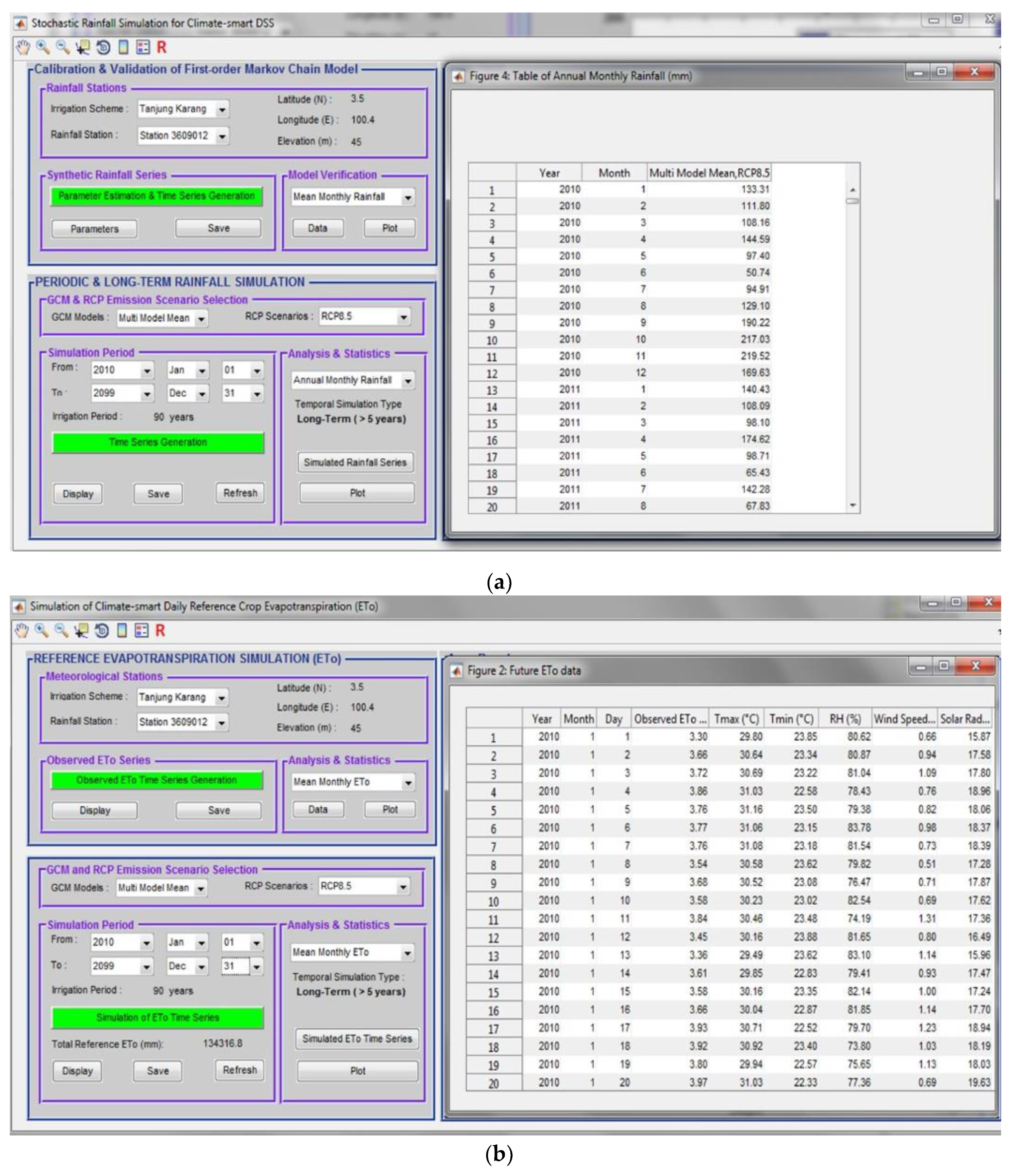
3.1. Projected Climatic Variables

Among the main climatic variables, which bring about the change in climate of an area are temperature and rainfall. They have greatest effect on the estimation of irrigation water demand [50]. Temperature is projected to increase due to climate change effects by an average of 1.18, 1.14, and 1.97 °C, respectively under RCPs 4.5, 6.0, and 8.5 compared to the baseline period. Similarly, the projected minimum temperature increase by 1.27, 1.21, and 2.08 °C for the same future periods. This culminated in the expectation that the basin would be warmer in the future, especially during the dry season months.

On the other hand, rainfall may slightly increase in the wet season (July–December) and decrease in the dry season (January–June) during the future period. The wet season average changes are projected to be 1.0%, 0.8%, and 2.4% under RCPs 4.5, 6.0, and 8.5 scenarios, respectively with a range of 0.2% for RCPs 4.5 and 6.0 in the 2050s to 2.7% for the RCP 8.5 in the 2080s. Whereas, the average changes for the dry season are −2.4%, −3.2%, and −3.7% under RCPs 4.5, 6.0, and 8.5 scenarios, respectively. Based on these findings, flood increases are likely to occur during the wet (main rice growing) season and so are some intermittent dry spells during the dry season. This difference in rainfall in both seasons needs to be taken into account in the scheme’s water resources planning.

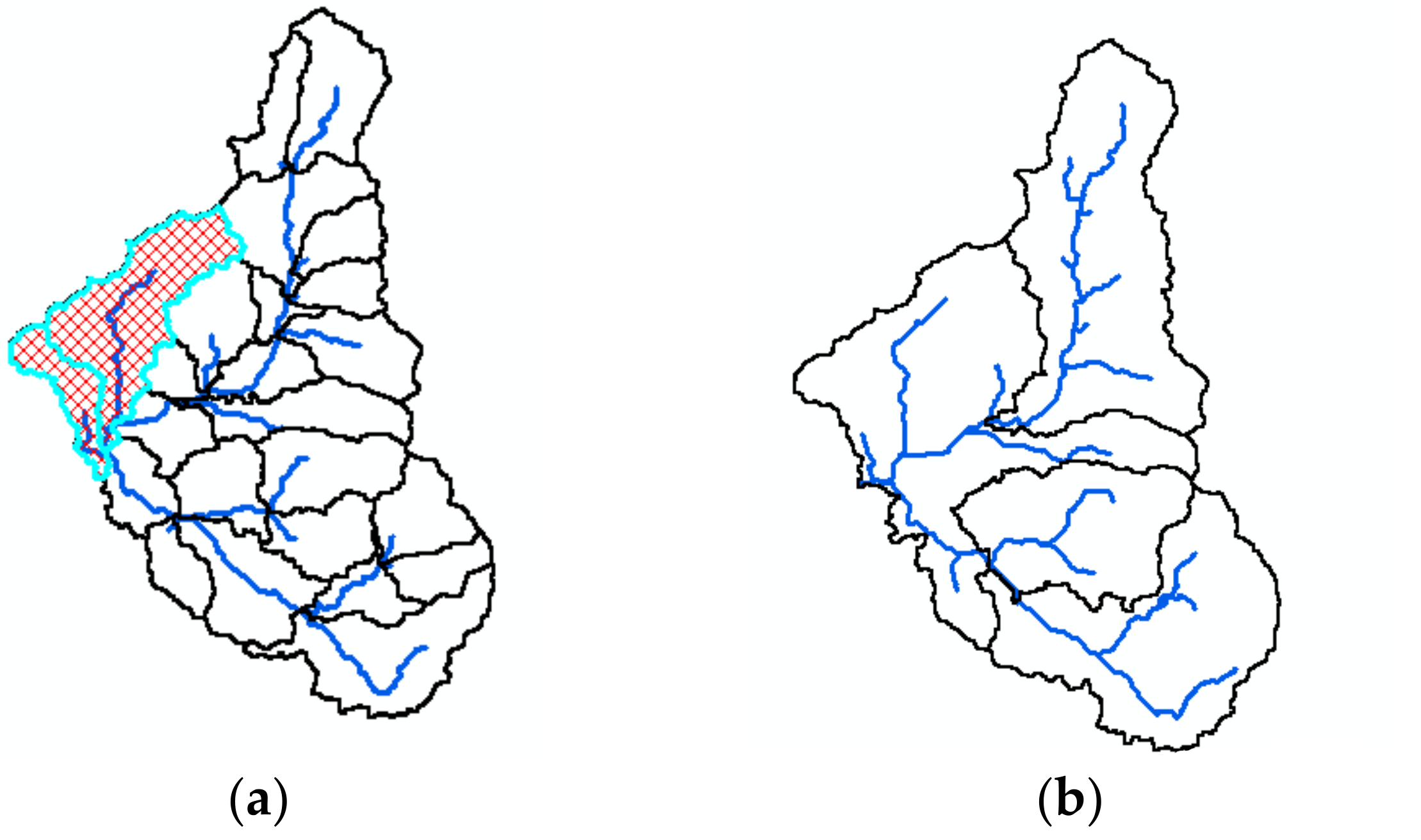
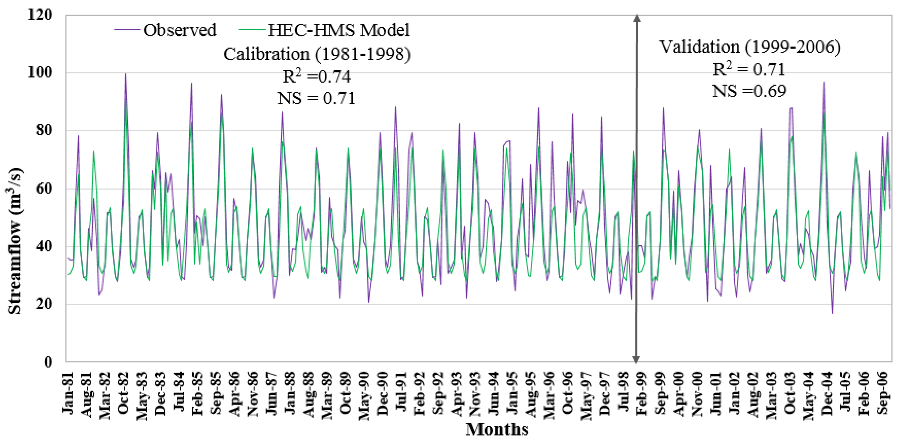
3.2. Hydrological Modeling

Monthly stream records of 30 years (1976–2006) were used for model evaluation. Out of the 30 years records, 18 years (1981–1998) was used for the calibration while 8 years (1999–2006) were used for the validation with 5 years warm up period in each. In both calibration and validation periods, the monthly observed and simulated discharges from the model were compared. Results of R², NSE, and PBIAS during the calibration and validation periods were 0.74, 0.71, and 4.21; and 0.71, 0.69, and 5.32, respectively. These results indicate a satisfactory simulation, as the values are greater than 0.5 [51]. The observed and simulated flows matched well during the calibration and validation periods as shown in Figure 6. However, there was under-prediction of some peak flows with much higher values for some months.

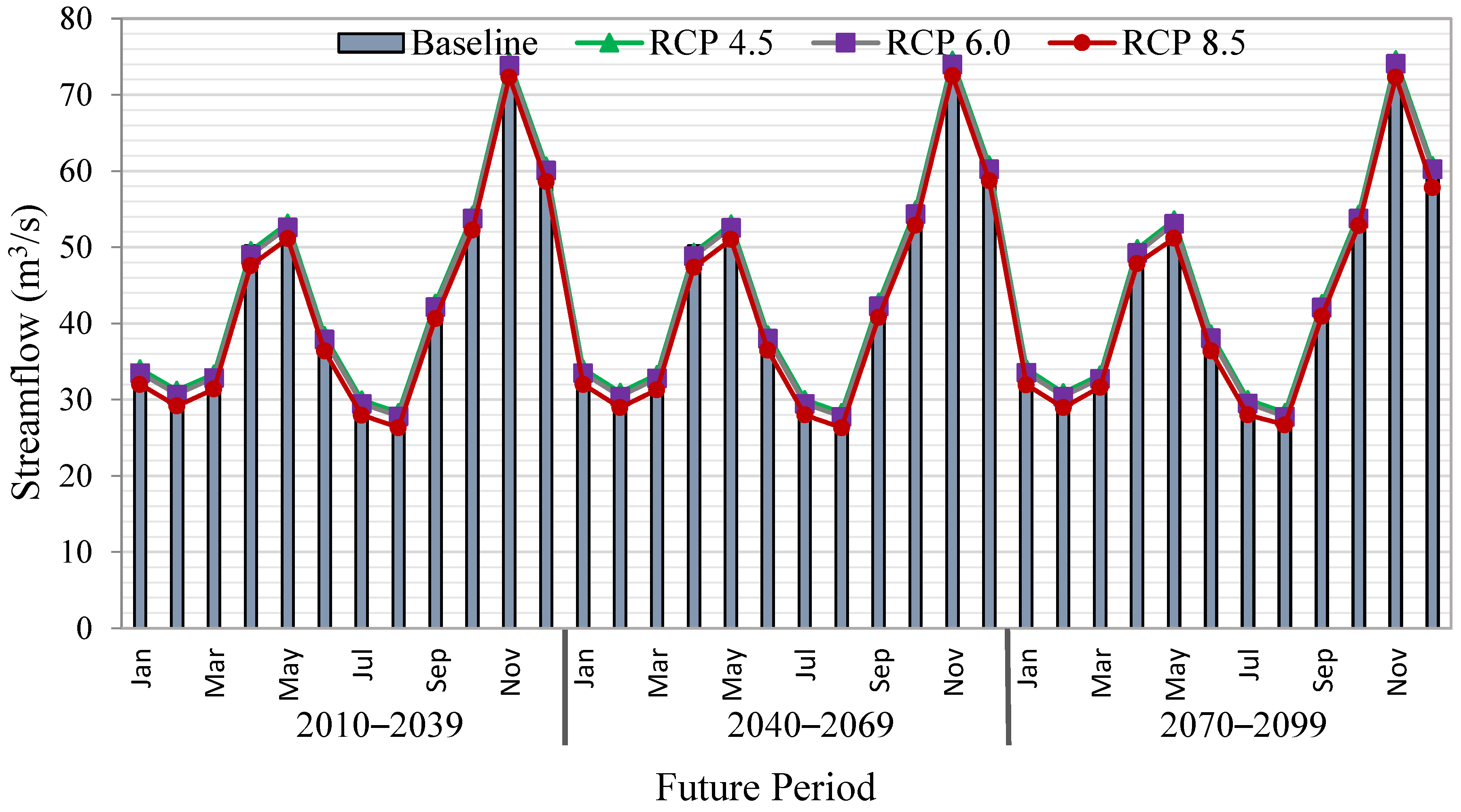
3.3. Future Changes in Streamflow at Bernam Basin Outlet

The validated HEC-HMS Model was used to assess the future changes in streamflow at the basin outlet. Climate change effects were assessed by combining all simulations of similar carbon emission scenarios for the three future periods using the ensemble of the 10 GCMs. The changes are the differences relative to the baseline period (1976–2005). The changes in future streamflow at Bernam river basin is more pronounced during the dry season period (Figure 7). This might be associated with the warmer temperature during the dry season usually, which consequently increases the rate of evapotranspiration more compared to wet season period, thus affects the future streamflow. The average changes under RCP 4.5, RCP 6.0, and RCP 8.5 are −0.40%, −1.68%, and −5.71%, respectively, during the dry season. In general, the future periods indicate a decreasing streamflow trend in this season, with a higher percentage (−5.94%) predicted in the 2080s under RCP 8.5 scenario. Similarly, in the wet season, streamflow decreases in all future periods except for RCP 4.5 where is expected to increase (0.36%). The average changes under RCP 6.0 and 8.5 are −0.67% and −3.83%, respectively. The changes in future streamflow at the Bernam River Basin would generally be more apparent during the dry season period. This may be connected with the warmer temperature during this time, thus affecting the future flow. The available water for supply to the scheme is largely reliant on the streamflow at the Basin outlet. A significant change in the future streamflow translates to the available irrigation supply. Therefore, the scheme is predicted to experience water shortage, particularly during the dry season period. This would then affect the water resources in the scheme, which could lead to adverse impacts on the overall crop production in the area. A Similar decrease in annual streamflow was observed by [5]. A decrease in annual streamflow in the wettest scenarios and decline in the driest scenarios was also reported by [52].

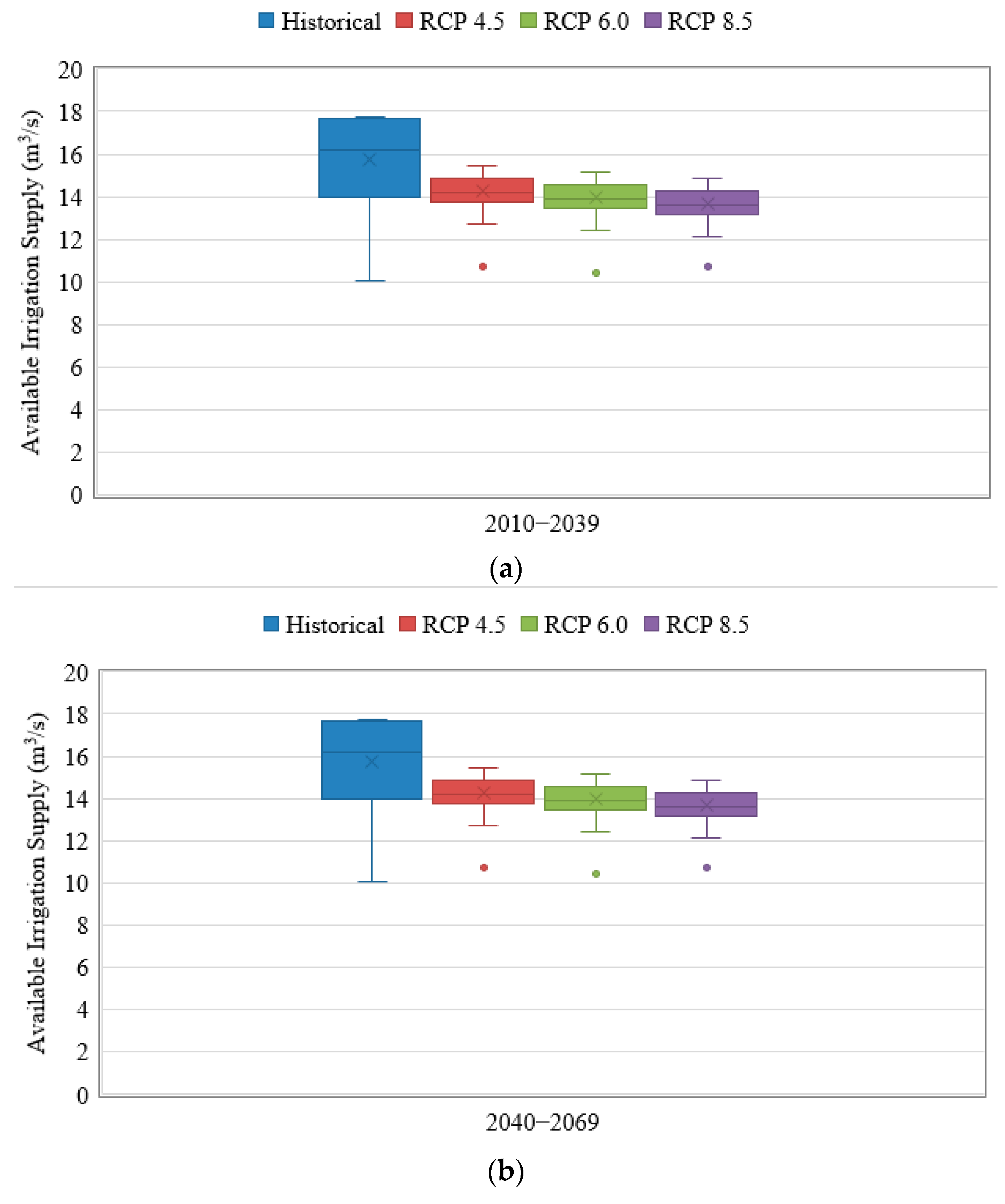
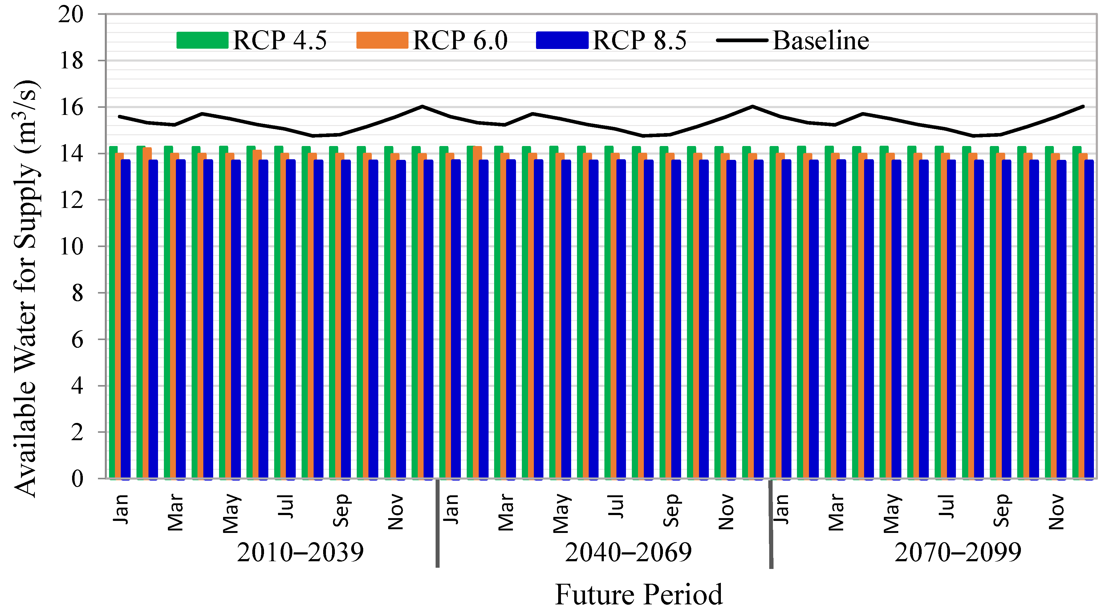
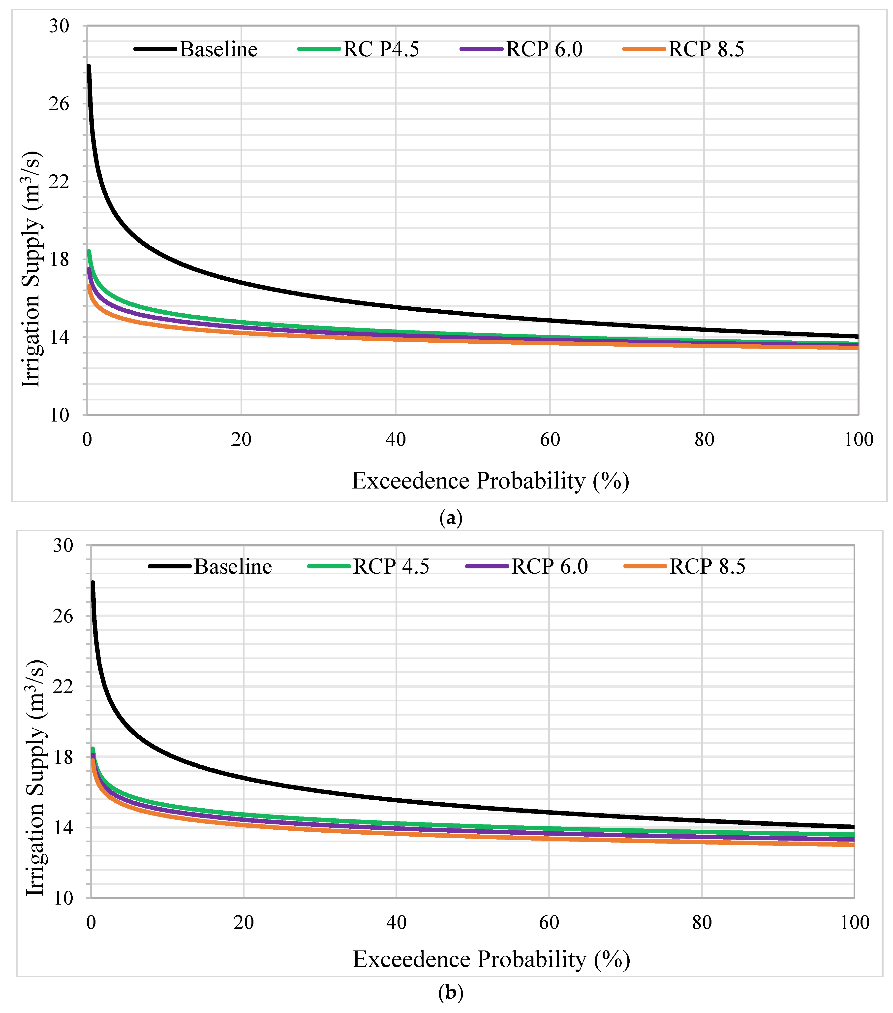
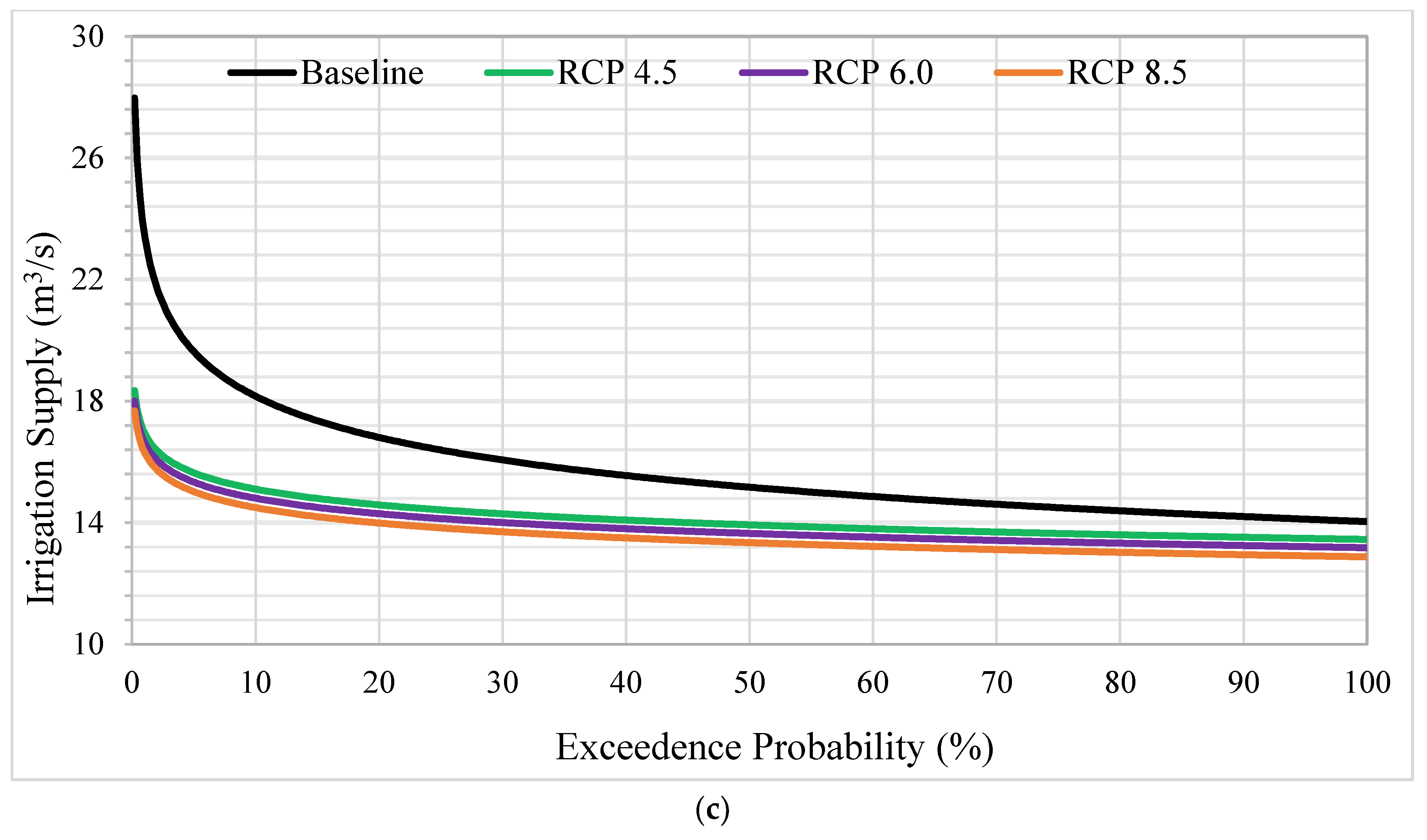
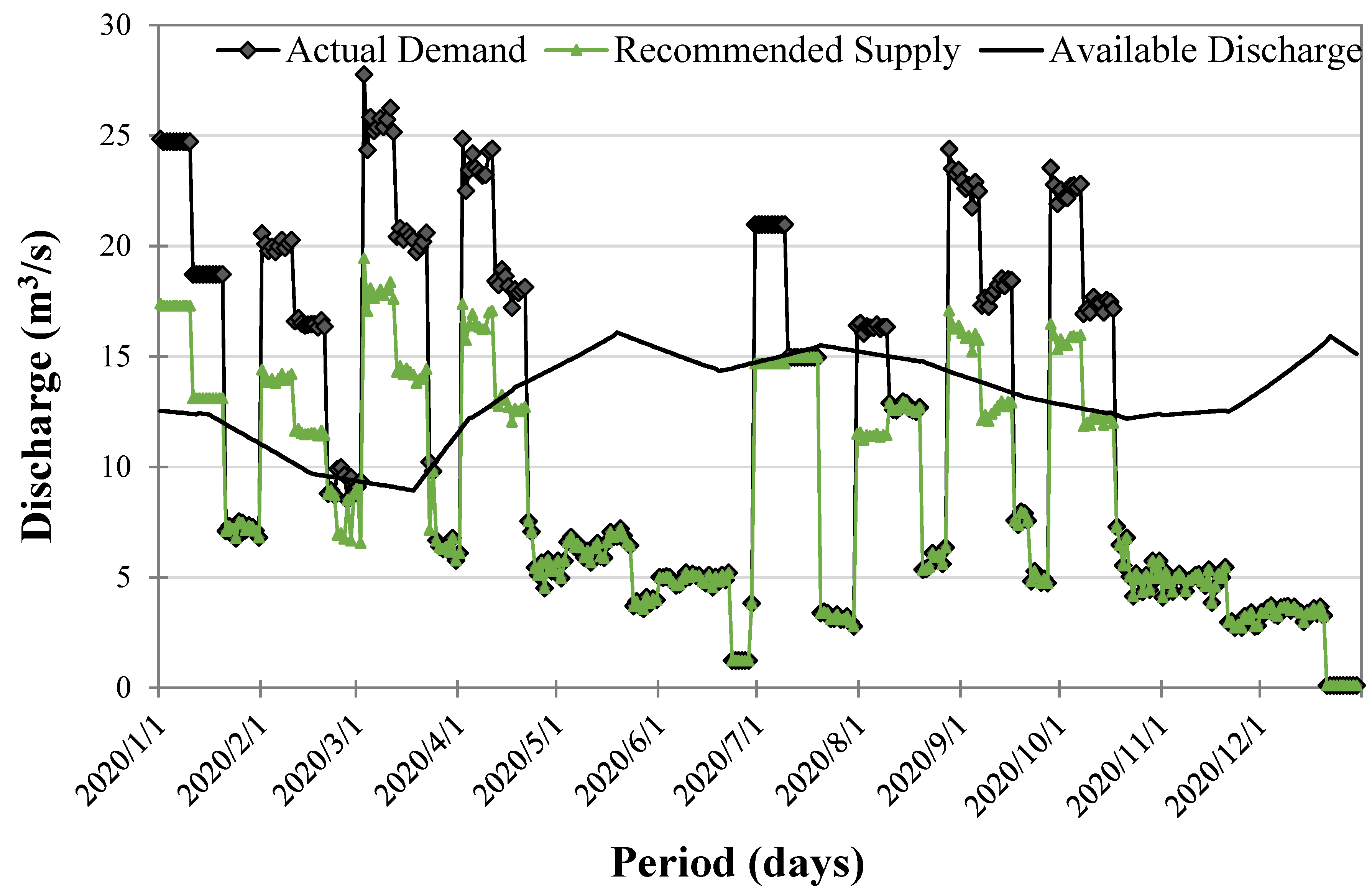
3.4. Projection of Available Supply for Irrigation under Climate Change

A DEM of the area was used to generate and extract the geometry of the river, starting from the water source at SKC gauging station to the TRH at the intake of the scheme. The river reach was divided into about 59 cross-sections, perpendicular to the flow direction from Upper Bernam watershed outlet to the TRH as shown in Figure 8.

The GIS extension of HEC-RAS model (HEC-GeoRAS) was used to extract the bathymetry of each cross-section, the distance between two adjacent cross-sections. Each section is represented by the coordinates (X,Y) where X (corresponding to station value), is the abscissa measured starting from a point chosen on one of banks and Y (corresponding to elevation value), is the ordinate measured starting from a horizontal plane of reference. The adjusted values of coefficient of Manning’s roughness used are 0.045 for the main channel and 0.05 for both left and right overbanks. The contraction coefficient was fixed to 0.1 and the coefficient of expansion was fixed to 0.3.

In both calibration and validation periods, the daily observed and simulated discharge from the model were compared. Results of R², NSE, and PBIAS during the calibration and validation periods were 0.73, 0.72, and 0.81 and 0.70, 0.65, and 1.79, respectively. These show that the simulation is satisfactory since the values are greater than 0.5 [51]. In addition, the model was able to optimally captured low and peak flows for most of the days. Figure 9 shows the projected annual available discharge for irrigation supply at the scheme intake. The available discharge depends on the streamflow from the basin outlet. The interquartile range, the median and average values of available water supply for the future years would be smaller than that of past years. The decrease in supply is more pronounced during the 2080s period under the RCP 8.5 scenario. The average supply for historical (1976–2005) period is 15.97 m³/s, which would decrease by 12%, 18%, and 21% under RCP 4.5, 6.0, and 8.5, respectively. Therefore, based on these findings, the projected available supply by the model for different scenario could be integrated with adaptive cropping patterns to enhance future water allocation. For instance, a recommended supply could be adopted, which enables proportionate distribution of water among the tertiary canals through proper control of the off-take structures gate. Thus, a factor can be introduced (considering the rice’s water-sensitive growth stages) to achieve an equitable supply. The factor depends on the management and operational decisions in the command area with respect to the available water for irrigation. With the advancement of irrigation season, the recommended irrigation supply (allowable supply based on available water) for tertiary canals is proposed. This adaptive strategy could be useful for most irrigation schemes operating on run-of the river, with limited or no water storage facility.

Figure 10 illustrates the average seasonal future changes in available supply for the wet/main irrigation season (July–December) and dry season (January–June) relative to the baseline period. The mean changes for RCPs 4.5, 6.0, and 8.5 are −7.94% (−7.86%), −10.30% (−9.84%), and −12.42% (−12.26%) during the dry (and main) seasons, respectively. Generally, the seasonal supply is projected to decrease for RCP 4.5, RCP 6.0, and RCP 8.5 scenarios. However, in all the future periods there will be a higher decrease during the dry season period under the worst-case scenario (RCP 8.5). This is expected because of decrease in rainfall and warmer temperature during the dry season, which increase the rate of evapotranspiration more compared to wet season period, and consequently change the future available supply.

Figure 11 shows the estimated flow duration curves for the available supply in response to the ensemble of 10 climate models and respective RCP scenarios. The 95th percentile supply (i.e., equaled or exceeded 95% of the time) for the 30-year simulation period projected to decrease by 3.17%, 3.53%, and 4.35%; 3.47%, 5.30%, and 7.51%; and 4.49%, 6.35%, and 8.74% in response to RCP 4.5, RCP 6.0, and RCP 8.5, respectively for 2020s, 2050s, and 2080s. This implies that the available supply of 14.12 m³/s obtainable in 95% or more of the time in the baseline period would decrease by the given percentages in the future for different scenario at similar percentile. Hence, the projected outputs show that available supply is more likely to decrease for all three RCPs with higher percentage under the worst-case scenario (RCP 8.5). In addition, there is a decreasing trend in available supply in the future periods, particularly in the late century (2080s). Therefore, based on the projected available supply, it may confirm that climate change will have impacts on hydrologic response of the basin and consequently on the scheme water resources. With increasing probability, the available supply would decrease due to climate change in the future periods and the balance of water resource structure would also change. This would adversely affect the inflow to and release at the intake of the scheme to meet the irrigation demand.

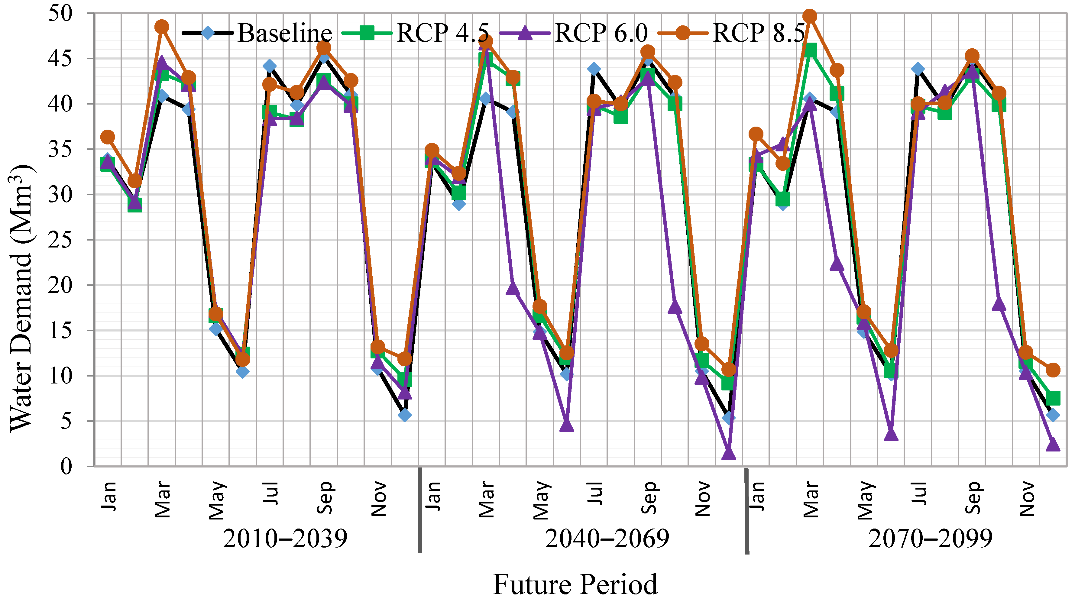
3.5. Water Demand Projection

The projected water demand using the ensemble and RCP scenarios indicated the scheme will require more irrigation water in the future (with higher rate under RCP 8.5) in the months of March and September during dry and wet seasons, respectively (Figure 12). This is because in March (during the dry season), ISA III is pre-saturated plus normal irrigations for ISAs I, II, and III, which require larger irrigation amount. In addition, in September (during wet season), ISA III is pre-saturated together with ISAs I, II, and III under normal irrigations. In the other hand, a less water demand is observed from May to June in the dry season period and from November to December in the wet season. Normal irrigations is only observed in these periods, which require lesser irrigation amount.

The estimated water demand during dry season under multi-model projections based on RCP 4.5, 6.0, and 8.5 scenarios indicate an increasing trend of water demand, with a higher increase (11.09%) anticipated in the late century (2080s) under the RCP 8.5 scenario. The average changes in this season are 5.59%, −5.75%, and 10.71% for RCPs 4.5, 6.0, and 8.5, respectively. Increasing water demand in the dry season is attributed to the rise in temperature and decrease in seasonal rainfall. For RCP4.5 (RCP8.5) scenarios, water demand is expected to decrease 2.6% (6.2%) during the wet season, respectively. Although the temperature is expected to rise in the wet season, the reason for the decrease in seasonal water demand is due to a substantial contribution from the effective rainfall following the wet season Northeast Monsoon rainfall, which compensates for the warmer periods. Climate change may not significantly affect water availability in the countries of South-East Asia because water demand will decrease due to increased rainfall [53]. Throughout the dry season the water demand in the scheme will vary considerably in the future over the months, and the rise in effective rainfall during the wet season will compensate for the high demand for dry seasonal water. Therefore, no irrigation is needed in the months of May and June. However, the major challenge will be to manage the monthly variability in irrigation water demand in the target area properly, failure of which the irrigation system would lead to much greater uncertainty as the project is a run-of-the-river irrigation scheme with limited storage facilities.

The project in Tanjung Karang Rice Irrigation is a run of the river (i.e., no water storage provided), which means the flowing water along the river to the scheme is either used or run as waste. Noticeably, the water supply to the scheme is not regulated based on the water demand. Irrigation supply is thus, observed to fluctuate along the seasons with over-supply in some periods and under-supply in other periods. It is projected that in future, the scheme would be over-supplied in January–February, May–June during dry season period, and November–December during wet season, with noticeable excess supplies in June and December (

Table 3. Projected excess/shortage water supply under RCP scenarios 4.5, 6.0, and 8.5 for the periods 2010–2039, 2040–2069, and 2070–2099.

Season	RCP 4.5			RCP 6.0			RCP 8.5
	2020s	2050s	2080s	2020s	2050s	2080s	2020s	2050s	2080s
Dry season
Jan	1.8	1.7	1.8	1.4	1.3	1.2	0.1	0.7	−0.1
Feb	2.5	1.9	2.2	2.0	0.9	−0.6	0.8	0.4	0.2
Mar	−1.9	−2.5	−2.9	−2.7	−3.5	−4.6	−4.5	−4.9	−6.5
Apr	−2.0	−2.2	−1.6	−2.3	6.4	5.3	−2.9	−2.9	−3.5
May	8.1	8.1	8.1	7.6	8.4	8.0	7.4	7.1	7.2
June	9.5	9.7	10.2	9.2	12.2	12.6	9.1	8.8	9.1
Wet Season
Jul	−0.34	−0.6	−0.6	−0.3	−0.8	−0.6	−2.0	−1.4	−1.2
Aug	−0.02	−0.2	−0.3	−0.4	−1.0	−1.5	−1.7	−1.3	−1.2
Sep	−2.22	−2.4	−2.4	−2.4	−3.6	−3.6	−4.2	−4.4	−4.7
Oct	−0.68	−0.7	−0.6	−0.9	7.4	7.3	−2.2	−2.2	−2.1
Nov	9.3	9.8	9.8	9.5	10.2	10.0	8.6	8.5	8.8
Dec	10.7	10.8	11.5	10.9	13.4	13.0	9.3	9.7	9.7

Note: Water supply > Water demand (Excess +), Water supply < Water demand (Shortage −).

). However, from March–April in dry season and July–October (except October in 2050s and 2080s for RCP 6.0) in wet season, a shortage supply is projected based on the irrigation demand for RCPs 4.5, 6.0, and 8.5. Since the project is a run of the river, a recommended supply could be adopted, which enables a proportionate distribution of water among the tertiary canals through proper control of diversion headworks. For effective irrigation water management, a good balance between water supply and demand needs to be achieved. This could be attained through operational actions, many of which require predictive models and instruments to be applied [54]. Therefore, the developed model could be integrated with adaptive cropping patterns to enhance the water allocation through the proper supply of the desired needed water in the scheme, thereby avoiding over-supply in the period of low demand and under-supply in the period of high demand.

The projected daily available discharges for irrigation supply, actual water demand, and recommended irrigation supply in response to the ensemble of 10 climate models with the worst-case scenario (RCP 8.5) from 1 January to 31 December 2020 is shown in Figure 13. It can be noted that the irrigation system was unable to satisfy the high water demand particularly in January, March–May in the dry-season and July, September–November in the wet-season due to shortage of water in the main canal. As a result, many farmers at the downstream do not usually receive supplies of irrigation in their fields. Noticeably, while shortages of water are experienced in some periods along the season, there are excess water in other periods, which run as waste. A study by [55] found that rice production and agricultural irrigation water use would be affected by potential risks on the future climate change. The highest environmental and agricultural sustainability index values are related to the incorporation of the change in crop pattern with improvement of the overall irrigation efficiency [56]. Climate change requires new approaches combining adaptation and mitigation strategies to realize the goal of sustainable development [57]. To assess water resource utilization many concepts have been applied for example, water footprint [55], a conception method by which indices of risk vis-à-vis drinking water was assessed, on the basis of a probability estimation methodology [58]. Furthermore, [57] analyzes the motivations driving a case study at water authority level using Information and Communication Technologies (ICTs) to support strategic management decisions involving risky choices.

A storage reservoir was recently built in the scheme, however, its capacity is inadequate. It is therefore necessary to construct reservoir(s) to store more water for future use. The storage capacity would be based on the projected discharge at the supply intake taking into account the streamflow from the water source. The excess water could be stored in the reservoir and use during the period of high demand. Finally, a proper assessment on future changes in rice production for the scheme is recommended, through investigations of how climate change impacts irrigation water planning and management for rice.

4. Conclusions

The HEC-HMS model was applied for the assessment of climate change impacts in future streamflow by using ensemble climate projections from 10 GCMs under RCP 4.5, RCP 6.0, and RCP 8.5 scenarios for adaptive water allocation at Tanjung Karang Rice Irrigation Scheme Malaysia. The changes in major rice farming (dry and wet) season results are reported. The changes are the differences relative to the baseline period (1976–2005) for the three 30-year defined future period (2020s, 2050s, and 2080s). Temperature is projected to increase; however, rainfall would decrease in the dry season and slightly increase in the main season. Compared with baseline streamflow records, the seasonal streamflow is projected to decrease for the three scenarios under the three future periods. However, in all the future periods there will be a higher decrease during the 2080s in the dry season period under the worst-case scenario (RCP 8.5). The interquartile range, the median and average values of available irrigation supply at the scheme for future years would be smaller than that of past years. The average irrigation supply for historical (1976–2005) period is 15.97 m³/s, which would decrease by 12%, 18%, and 21% under RCP 4.5, 6.0, and 8.5, respectively.

The irrigation supply is observed to fluctuate along the seasons with over-supply in some periods and under-supply in other periods with respect to the needed supply by the scheme. Therefore, the developed model could be integrated with adapted cropping patterns to enhance the water allocation through the proper supply of the desired needed water in the scheme, thereby avoiding over-supply in the period of low demand and under-supply in the period of high demand.

References

1. Huang, H.; Han, Y.; Jia, D. Impact of climate change on the blue water footprint of agriculture on a regional scale. Water Sci. Technol. Water Supply 2019, 19, 52–59. [Google Scholar] [CrossRef]
2. Kamal, M.R.; Iqbal, M.; Mojid, M.A.; Amin, M.A.M.; Hin, L.S. Optimization of equitable irrigation water delivery for a large-scale rice irrigation scheme. IJABE 2018, 11, 160–166. [Google Scholar]
3. Huabin, Z.; Wei, Z.; Qimin, C.; Yuanwei, C.; Qiyuan, T. Water-saving irrigation practices for rice yield information and nitrogen use efficiency under sub-tropical monsoon climate. Water Supply 2019, 19, 2485–2493. [Google Scholar] [CrossRef]
4. Zhang, J.; Fu, Y.C.; Shi, W.L.; Guo, W.X. A method for estimating watershed restoration feasibility under different treatment levels. Water Sci. Technol. Water Supply 2017, 17, 1232–1240. [Google Scholar] [CrossRef] [Green Version]
5. Chien, H.; Yeh, P.J.F.; Knouft, J.H. Modeling the potential impacts of climate change on streamflow in agricultural watersheds of the Midwestern United States. J. Hydrol. 2013, 491, 73–88. [Google Scholar] [CrossRef]
6. Sezen, C.; Šraj, M.; Medved, A.; Bezak, N. Investigation of rain-on-snow floods under climate change. Appl Sci. 2020, 10, 1242. [Google Scholar] [CrossRef]
7. Bruijnzeel, L. Predicting the hydrological impacts of land cover transformation in the humid tropics: The need for integrated research. In Amazonian Deforestation and Climate, 1st ed.; Gash, J.H.C., Ed.; John Wiley & Sons: New York, NY, USA, 1996; Volume 1, pp. 15–55. [Google Scholar]
8. Iqbal, M.; Kamal, M.R.; Che Man, H.; Wayayok, A. HYDRUS-1D simulation of soil water dynamics for sweet corn under tropical rainfed condition. Appl. Sci. 2020, 10, 1219. [Google Scholar] [CrossRef]
9. Li, X.; Gao, X.; Chang, Y.; Mu, D.; Liu, H.; Sun, Z.; Guo, J. Water storage variations and their relation to climate factors over Central Asia and surrounding areas over 30 years. Water Sci. Technol. Water Supply 2017, 18, 1564–1580. [Google Scholar] [CrossRef] [Green Version]
10. Wu, Y.; Zhang, G.; Shen, H.; Xu, Y.J. Nonlinear response of streamflow to climate change in high-latitude regions: A case study in headwaters of Nenjiang river basin in China’s far northeast. Water 2018, 10, 294. [Google Scholar] [CrossRef]
11. Givati, A.; Thirel, G.; Rosenfeld, D.; Paz, D. Climate change impacts on streamflow at the upper Jordan River based on an ensemble of regional climate models. J. Hydrol. Reg. Stud. 2019, 21, 92–109. [Google Scholar] [CrossRef]
12. Guo, Q.; Han, Y.; Yang, Y.; Fu, G.; Li, J. Quantifying the impacts of climate change, coal mining and soil and water conservation on streamflow in a coal mining concentrated watershed on the Loess Plateau, China. Water 2019, 11, 1054. [Google Scholar] [CrossRef]
13. Shrestha, S.; Sharma, S.; Gupta, R.; Bhattarai, R. Impact of global climate change on stream low flows: A case study of the great Miami river watershed, Ohio, USA. IJABE 2019, 12, 84–95. [Google Scholar] [CrossRef]
14. Gaertner, B.; Fernandez, R.; Zegre, N. Twenty-first century streamflow and climate change in forest catchments of the central appalachian mountains region, US. Water 2020, 12, 453. [Google Scholar] [CrossRef]
15. Mu, X.; Wang, H.; Zhao, Y.; Liu, H.; He, G.; Li, J. Streamflow into Beijing and its response to climate change and human activities over the period 1956–2016. Water 2020, 12, 622. [Google Scholar] [CrossRef] [Green Version]
16. Dlamini, N.S.; Rowshon, M.K.; Amin, M.S.M.; Mohd, M.S.F. Modeling potential impacts of climate change on streamflow using projections of the 5th assessment report for the bernam river basin, Malaysia. Water 2017, 9, 226. [Google Scholar] [CrossRef]
17. Kabiri, R.; Bai, V.R.; Chan, A. Assessment of hydrologic impacts of climate change on the runoff trend in Klang Watershed, Malaysia. Environ. Earth Sci. 2015, 73, 27–37. [Google Scholar] [CrossRef]
18. Shrestha, S.; Khatiwada, M.; Babel, M.S.; Parajuli, K. Impact of climate change on river flow and hydropower production in Kulekhani hydropower project of Nepal. Environ. Proc. 2014, 1, 231–250. [Google Scholar] [CrossRef]
19. Meenu, R.; Rehana, S.; Mujumdar, P. Assessment of hydrologic impacts of climate change in Tunga-Bhadra river basin, India with HEC-HMS and SDSM. Hydrol. Proc. 2013, 27, 1572–1589. [Google Scholar] [CrossRef]
20. Nguyen, Q.D.; Roussey, C.; Poveda-Villalón, M.; Vaulx, C.d.; Chanet, J.P. Development experience of a context-aware system for smart irrigation using CASO and IRRIG ontologies. Appl. Sci. 2020, 10, 1803. [Google Scholar] [CrossRef] [Green Version]
21. NAWABS. National Water Balance Management System. Bagi Lembangan Sungai Bernam. Progress Report 2018. Available online: http://nawabs.water.gov.my/ (accessed on 21 May 2020).
22. Min, G.K.; Park, S.W. Combined simulation-optimization model for assessing irrigation water supply capacities of reservoirs. J. Irrig. Drain. Eng. 2014, 140. [Google Scholar] [CrossRef]
23. Clemmens, A.J.; Holly, F.M., Jr.; Schuurmans, W. Description and evaluation of program: DUFLOW (ASCE). J. Irrig. Drain. Eng. 1993, 119, 724–734. [Google Scholar] [CrossRef]
24. Schuurmans, W. Description and evaluation of program MODIS (ASCE). J. Irrig. Drain. Eng. 1993, 119, 735–742. [Google Scholar] [CrossRef]
25. Rogers, D.C.; Merkley, G.P. Description and evaluation of program USM (ASCE). J. Irrig. Drain. Eng. 1993, 119, 693–702. [Google Scholar] [CrossRef]
26. Singh, R.; Refsgaard, J.C.; Yde, L.; Jørgensen, G.H.; Thorsen, M. Hydraulic-hydrologicalsimulations of canal-command for irrigation water management. Irrig. Drain. Syst. 1997, 11, 185–213. [Google Scholar] [CrossRef]
27. Shahrokhnia, M.; Javan, M. Performance assessment of Doroodzan irrigation network by steady state hydraulic modeling. Irrig. Drain. Syst. 2005, 19, 189–206. [Google Scholar] [CrossRef]
28. Rowshon, M.K.; Mojid, M.A.; Amin, M.S.M.; Azwan, M.; Yazid, A.M. Improving irrigation water delivery performance of a large-scale rice irrigation scheme. J. Irrig. Drain. Eng. 2014, 140. [Google Scholar] [CrossRef]
29. Rowshon, M.; Amin, M.; Shariff, A.M. GIS user-interface based irrigation delivery performance assessment: A case study for Tanjung Karang rice irrigation scheme in Malaysia. Irrig. Drain. Syst. 2011, 25, 97–120. [Google Scholar] [CrossRef]
30. Ghosh, S.; Mujumdar, P. Nonparametric methods for modeling GCM and scenario uncertainty in drought assessment. Water Resour. Res. 2007, 43. [Google Scholar] [CrossRef]
31. New, M.; Hulme, M. Representing uncertainty in climate change scenarios: A Monte-Carlo approach. Integr. Assess. 2000, 1, 203–213. [Google Scholar] [CrossRef]
32. Rowshon, M.; Dlamini, N.; Mojid, M.; Adib, M.; Amin, M.; Lai, S. Modeling climate-smart decision support system (CSDSS) for analyzing water demand of a large-scale rice irrigation scheme. Agric. Water Manag. 2019, 216, 138–152. [Google Scholar] [CrossRef]
33. Abatzoglou, J.T.; Brown, T.J. A comparison of statistical downscaling methods suited for wildfire applications. Int. J. Clim. 2012, 32, 772–780. [Google Scholar] [CrossRef]
34. Fang, G.; Yang, J.; Chen, Y.; Zammit, C. Comparing bias correction methods in downscaling meteorological variables for a hydrologic impact study in an arid area in China. Hydrol. Earth Syst. Sci. 2015, 19, 2547–2559. [Google Scholar] [CrossRef] [Green Version]
35. Priestley, C.H.B.; Taylor, R. On the assessment of surface heat flux and evaporation using large-scale parameters. Monthly Weather Rev. 1972, 100, 81–92. [Google Scholar] [CrossRef]
36. USACE. Hydrologic Modeling System HEC-HMS: Technical Reference Manual; CPD-74B; Hydrologic Engineering Center: Davis, CA, USA, 2000.
37. Babel, M.S.; Bhusal, S.P.; Walid, S.M. Climate change and water resources in the Bagmati River, Nepal. Theor. Appl. Climatol. 2014, 115, 639–654. [Google Scholar] [CrossRef]
38. Bui, C. Application of HEC-HMS 3.4 in Estimating Streamflow of the Rio Grande under Impacts of Climate Change. Master’s Thesis, University of New Mexico, Albuquerque, NM, USA, 2011. [Google Scholar]
39. Halwatura, D.; Najim, M. Application of the HEC-HMS model for runoff simulation in a tropical catchment. Environ. Model Softw. 2013, 46, 155–162. [Google Scholar] [CrossRef]
40. Griffin, R.H. Risk-Based Analysis for Flood Damage Reduction Studies; EM 1110-2-1417; Department of the Army: Washington, DC, USA, 1994; Volume 5, p. 5.
41. USACE-HEC. Hydraulic Reference Manual; US Army Corps of Engineers: Davis, CA, USA, 2016.
42. Chow, V.T. Open Channel Hydraulics; McGraw-Hill Book Company: New York, NY, USA, 1959. [Google Scholar]
43. Van Liew, M.; Arnold, J.; Garbrecht, J. Hydrologic simulation on agricultural watersheds: Choosing between two models. Trans. ASAE 2003, 46, 1539. [Google Scholar] [CrossRef]
44. Nash, J.E.; Sutcliffe, J.V. River flow forecasting through conceptual models, part 1-A discussion of principles. J. Hydrol. 1970, 10, 282–290. [Google Scholar] [CrossRef]
45. Gupta, H.V.; Sorooshian, S.; Yapo, P.O. Status of automatic calibration for hydrologic models: Comparison with multilevel expert calibration. J. Hydrol. Eng. 1999, 4, 135–143. [Google Scholar] [CrossRef]
46. Chan, C.; Cheong, A. Seasonal weather effects on crop evapotranspiration and rice yield. J. Trop. Agric. Food Sci. 2001, 29, 77–92. [Google Scholar]
47. Allen, R.G.; Pereira, L.S.; Raes, D.; Smith, M. Crop Evapotranspiration-Guidelines for Computing Crop Water Requirements-FAO Irrigation and Drainage Paper 56; FAO: Rome, Italy, 1998; Volume 300, p. D05109. [Google Scholar]
48. Dlamini, N.; Rowshon, M.; Saha, U.; Lai, S.; Fikri, A.Z.; Zubaidi, J. Simulation of future daily rainfall scenario using stochastic rainfall generator for a rice-growing irrigation scheme in Malaysia. Asian J. Appl. Sci. 2015, 3, 492–506. [Google Scholar]
49. IADA. Final Report: Kajian Keberkesanan Taliair Tersier Di Seluruh Kawasan IADA Barat Laut Selangor. 2018. Available online: https://iadabls.moa.gov.my/sejarah (accessed on 21 May 2020).
50. Goodarzi, M.; Eslamian, S. Performance evaluation of linear and nonlinear models for the estimation of reference evapotranspiration. Int. J. Hydrol. Sci. Technol. 2018, 8, 1–15. [Google Scholar] [CrossRef]
51. Moriasi, D.N.; Arnold, J.G.; Van Liew, M.W.; Bingner, R.L.; Harmel, R.D.; Veith, T.L. Model evaluation guidelines for systematic quantification of accuracy in watershed simulations. Trans. ASABE 2007, 50, 885–900. [Google Scholar] [CrossRef]
52. Arnell, N.; Reynard, N. The effects of climate change due to global warming on river flows in Great Britain. J. Hydrol. 1996, 183, 397–424. [Google Scholar] [CrossRef]
53. Tukimat, N.; Harun, S.; Shahid, S. Modeling irrigation water demand in a tropical paddy cultivated area in the context of climate change. J. Water Res. Plan. Manag. 2017, 143. [Google Scholar] [CrossRef]
54. De Souza Groppo, G.; Costa, M.A.; Libânio, M. Predicting water demand: A review of the methods employed and future possibilities. Water Supply 2019, 19, 2179–2198. [Google Scholar] [CrossRef]
55. Yang, M.; Xiao, W.; Zhao, Y.; Li, X.; Huang, Y.; Lu, F.; Hou, B.; Li, B. Assessment of potential climate change effects on the rice yield and water footprint in the Nanliujiang catchment, China. Sustainability 2018, 10, 242. [Google Scholar] [CrossRef]
56. Ahmadaali, J.; Barani, G.A.; Qaderi, K.; Hessari, B. Analysis of the effects of water management strategies and climate change on the environmental and agricultural sustainability of Urmia Lake Basin, Iran. Water 2018, 10, 160. [Google Scholar] [CrossRef] [Green Version]
57. Cavazza, F.; Galioto, F.; Raggi, M.; Viaggi, D. The role of ICT in improving sequential decisions for water management in agriculture. Water 2018, 10, 1141. [Google Scholar] [CrossRef]
58. Rak, J.R.; Pietrucha-Urbanik, K. An approach to determine risk indices for drinking water–study investigation. Sustainability 2019, 11, 3189. [Google Scholar] [CrossRef] [Green Version]
Figure 1. View of the Location of Tanjung Karang Rice Irrigation Scheme in Malaysia [29].
Applsci 10 04885 g001
Figure 2. Framework for the adaptive water allocation under climate change.
Applsci 10 04885 g002
Figure 3. Windows for downscaling climatic variables time-series (2010–2099): (a) downscaling daily rainfall generation and (b) downscaling meteorological variables.
Applsci 10 04885 g003
Figure 4. Hydrologic Engineering Corps Hydrologic Modeling System (HEC-HMS) model development processes for upper Bernam river watershed: (a) basin merge, (b) basin river network, (c) HMS-node, and (d) HMS basin model.
Applsci 10 04885 g004aApplsci 10 04885 g004b
Figure 5. Hydrologic Engineering Centers River Analysis System (HEC-RAS) model setup for simulation of available canal flow.
Applsci 10 04885 g005
Figure 6. Simulated and observed monthly discharge for Bernam river basin during calibration and validation periods.
Applsci 10 04885 g006
Figure 7. Projected mean monthly streamflow for three future periods of 2010–2039, 2040–2069, and 2070–2099 relative to the baseline period of 1976–2005 using three Representative Concentration Pathway (RCP) scenarios (RCPs 4.5, 6.0, and 8.5).
Applsci 10 04885 g007
Figure 8. River geometry traits at the study location: (a) view of conveyance system from Bernam River Headworks (BRH) to Tengi River Headworks (TRH) (Map Data©Google Map, 2019); (b) cross-sections at Bernam River/Feeder canal; and (c) cross-sections at Tengi River.
Applsci 10 04885 g008
Figure 9. The projected ensemble irrigation supply under RCPs to the historical period: (a) 2020s, (b) 2050s, and (c) 2080s.
Applsci 10 04885 g009aApplsci 10 04885 g009b
Figure 10. Projected ensemble mean monthly supply and future changes under RCPs (RCPs 4.5, 6.0, and 8.5) for three future periods of 2010–2039, 2040–2069, and 2070–2099 relative to the baseline period of 1976–2005.
Applsci 10 04885 g010
Figure 11. Flow duration curve for ensemble irrigation supply under RCPs with respect to baseline period of 1976–2005: (a) 2020s, (b) 2050s, and (c) 2080s.
Applsci 10 04885 g011aApplsci 10 04885 g011b
Figure 12. Projected mean monthly water demand from multi-models with three RCP scenarios for future periods of 2010–2039, 2040–2069, and 2070–2099 relative to baseline period of 1976–2005.
Applsci 10 04885 g012
Figure 13. Projected daily available discharges for irrigation supply, actual water demand and recommended irrigation supply from multi-models for RCP 8.5 scenario from 1 January to 31 December 2020.
Applsci 10 04885 g013