Identification of the Dynamic Parameters of a Parallel Kinematics Mechanism with Prismatic Joints by Considering Varying Friction


1
Khalifa University Center for Autonomous Robotic Systems (KUCARS), Khalifa University of Science and Technology, P.O. Box 127788, Abu Dhabi, UAE
2
Mechanical Engineering Department, Khalifa University of Science and Technology, P.O. Box 127788, Abu Dhabi, UAE
*
Author to whom correspondence should be addressed.
Appl. Sci. 2020, 10(14), 4820; https://doi.org/10.3390/app10144820
Submission received: 8 June 2020
/
Revised: 6 July 2020
/
Accepted: 9 July 2020
/
Published: 14 July 2020
(This article belongs to the Special Issue Advances in Mechanical Systems Dynamics 2020)
Abstract
:This study proposed a novel approach for the offline dynamic parameter identification of parallel kinematics mechanisms in which the friction is significant and varying. Since the friction is significant, it should be incorporated to provide an accurate dynamic model. Furthermore, the varying normal forces as a result of the changing posture of the mechanism lead to varying friction forces, specifically varying static and Coulomb friction forces. By considering this variation, the static and Coulomb friction parameters are identified as coefficients instead of forces. A bound-constrained optimization technique using an iterative global search tool was employed in this work to minimize the residual errors while maintaining the physical feasibility of the solutions. Moreover, the friction was modeled by using the nonlinear Stribeck friction model since a linear friction model was not sufficient, whereas the variation of the friction followed the variation of the normal forces, which were evaluated through the Lagrange multipliers in the constrained dynamic model of the mechanism. The solutions obtained were verified by using some trajectories that were different from those used in the identification.
1. Introduction
The dynamic parameters of a rigid body system typically consist of the inertial and friction parameters. In a system where its inertial parameters are very dominant and its friction parameters are relatively very small, the friction parameters can be neglected in the identification. However, when the friction is significant, one should incorporate it in the dynamics, and accordingly include the friction parameters in the identification. Otherwise, the corresponding dynamic model is not adequate to capture the real dynamics. An identification usually estimates the inertial parameters as the so-called barycentric parameters, which consist of the masses, the first moments of inertia, and the moments of inertia relative to the origin of the component frames. Upon obtaining the masses and the first moments of inertia, one can easily obtain the centers of masses (COMs). The moments of inertia relative to the COM can be obtained from the moments of inertia relative to the component frame by utilizing the Huygens–Steiner theorem, which is commonly called the parallel axis theorem.
The dynamics of a mechanism can typically be modeled as a linear system in terms of the dynamic parameters. As a result, linear least squares can be conveniently used to identify the dynamic parameters [1]. Based on measurements along a certain exciting trajectory, an overdetermined linear system can be composed, and subsequently, the dynamic parameters can be estimated by using the closed-form linear least squares solution, which involves the evaluation of the pseudo-inverse of the observation matrix. In this case, accurate estimates of the dynamic parameters can only be obtained if the observation matrix has a full rank. In fact, the observation matrix is often rank-deficient. In such a case, a numerical or symbolic mathematical treatment is commonly performed to transform the rank-deficient observation matrix into a full-rank one. This results in a new full-ranked linear system with a reduced size. As the rank-deficiency implies a linear dependency among some dynamic parameters, the reduced linear system can only present the dynamic parameters as linear combinations of the parameters, commonly known as the base parameters.
When friction is included, the linear least squares technique can only incorporate a linear friction model. The use of nonlinear optimization techniques can overcome this issue. There are at least three main advantages of this approach. First, one can directly utilize the nonlinear dynamic model, including a nonlinear friction model, to identify the dynamic parameters instead of transforming the nonlinear dynamic model into a linear model, as described earlier. In other words, one can directly use the nonlinear inverse dynamics for identification. The second advantage is the capability of this approach to provide the dynamic parameters as lonely parameters, i.e., not as linear combinations. The third advantage of this approach is the flexibility to identify the dynamic parameters as either the standard parameters or the barycentric parameters. One of the commonly used nonlinear optimization techniques is the nonlinear least squares, in which the Jacobian of the system with respect to the dynamic parameters should be evaluated. While in the linear identification method, the observation matrix should be full-rank to obtain a trustworthy solution from the linear least squares, in a similar fashion, the system Jacobian matrix should be full-rank to get a trustworthy solution from the nonlinear least squares.
Although the linear least squares methods applied to a full-rank reduced linear system or the nonlinear least squares applied to a nonlinear system with a full-rank system Jacobian matrix can theoretically give a trustworthy solution, in practice, it is very likely that it cannot give a physically feasible solution due to the presence of measurement noise and/or the inadequacy of the dynamic model. The authors noticed that both the linear and nonlinear least squares techniques can retrieve synthesized (simulated) measurements but fail to provide physically feasible estimates when real, noisy measurements are used. For that reason, constrained optimization is used in this work to obtain a physically feasible solution. A similar approach has been used by Farhat et al. [2] and Thanh et al. [3], who respectively used a constrained optimization algorithm and a direct search to identify the dynamic parameters of a parallel kinematics mechanism (PKM). Moreover, Poignet et al. [4] used interval analysis to identify the dynamic parameters of an H4 manipulator, which is a three-translational and one-rotational (3T1R) PKM.
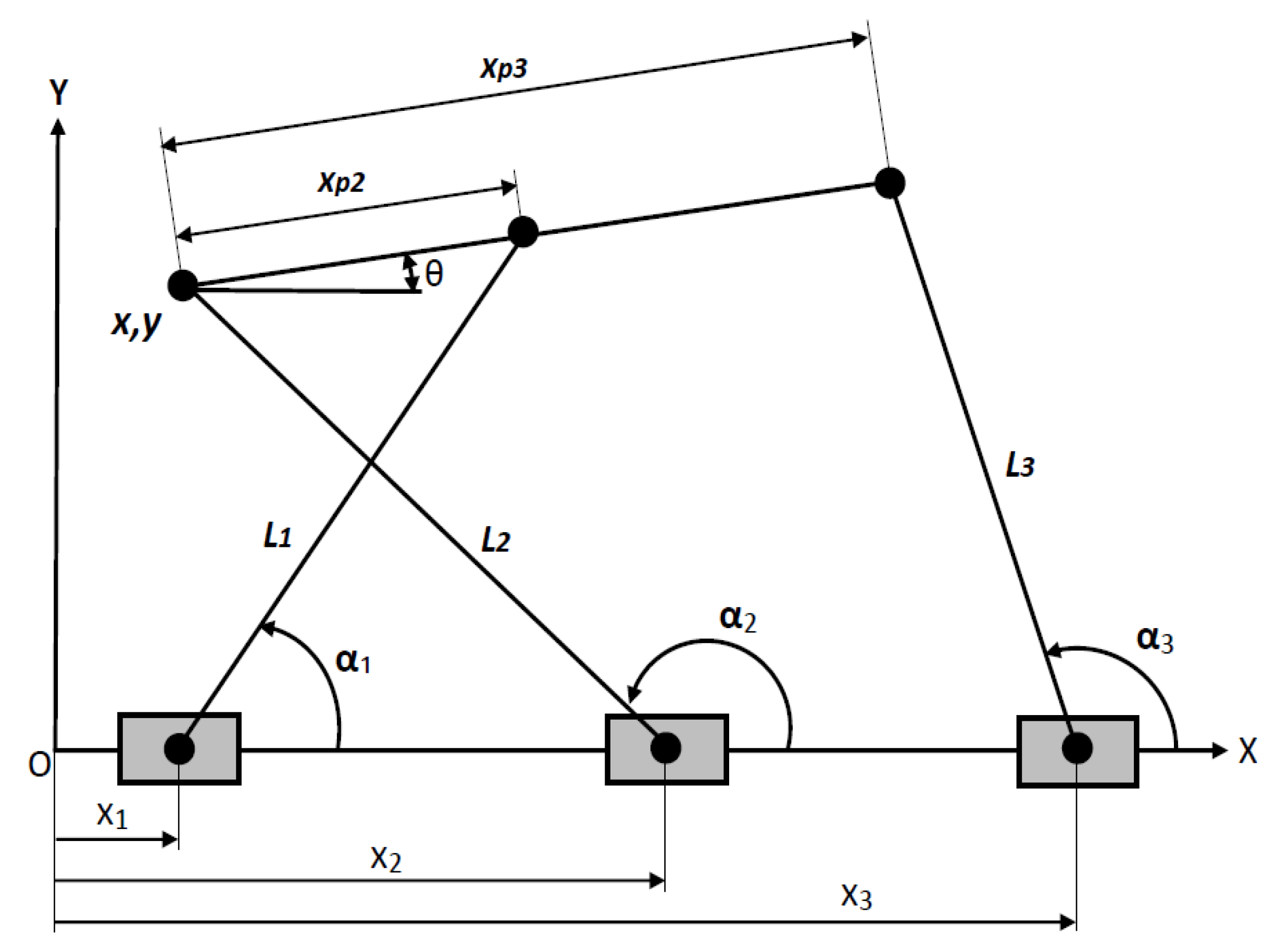
Furthermore, this work considered a PKM with significant friction due to the presence of sliding (prismatic) joints subject to a significant load. This load was comprised of a constant gravity load and varying reaction forces. Different from a system having sliding joints with constant normal forces, such as in Pan et al. [5], in this work, the total load resulted in varying normal forces, and therefore, varying friction forces. In fact, the normal forces varied because of the changing posture of the PKM. This behavior applies to all types of PKMs, regardless of the magnitude of the variation. However, to the authors’ knowledge, there has been no published work on the dynamic parameter identification of PKMs that considers the variation of the friction forces. Moreover, most of the works, including References [3,4,6,7,8,9,10,11,12,13], have also used a linear friction model to enable the use of linear least squares algorithms, including the unweighted linear least squares, weighted linear least squares, and total linear least squares algorithms, as the identification tool. Recently, Farhat et al. [2] used a nonlinear friction model to identify the dynamic parameters of a 3RPS (3 Revolute-Prismatic-Spherical joint topology) PKM. Furthermore, Briot and Gautier [13] identified not only the inertial and friction parameters of an Orthoglide PKM but also its drive gains. All of the mentioned works considered the friction in the PKMs constant. This study investigated the identification of the dynamic parameters of a PKM by considering nonlinear, varying friction. In short, this work proposed an approach for the identification of a PKM with noisy measurements, as well as nonlinear and varying friction. In this work, the dynamics were derived by using a Lagrange approach. A set of constraint equations corresponding to the required Lagrange multipliers were formulated. These Lagrange multipliers corresponded to the reaction forces at all joints, including the active and passive ones. Since the friction on the active, prismatic joints were assumed to be much more significant than that on the passive joints, only the former was considered. To describe the approach, a non-symmetric planar 3PRR (3 Prismatic-Revolute-Revolute joint topology) PKM [14,15], as shown in Figure 1, was considered as the study case. This paper is organized as follows. First, the inverse dynamics of the mechanism at hand with and without friction are derived and the friction model is presented. Second, the identification technique is discussed, where the discussion includes the optimization of the exciting trajectory and the physical feasibility of the estimation. Finally, the identification results are discussed.
2. Dynamic Model
The dynamics of a mechanism can be modeled by using different sets of generalized coordinates. Since a PKM has constrained dynamics, the dynamic model is usually modeled by using a set of redundant generalized coordinates that can be divided into independent and dependent coordinates. In the mechanism at hand, twelve generalized coordinates, as shown in Rodríguez et al. [11] are used. For more convenience, the Cartesian coordinates of the moving platform x, y, and θ are used to represent the pose of the manipulator. Since the mechanism has three degrees of freedom without a kinematic redundancy, only three coordinates are independent, while the remaining coordinates are dependent. The closed-loop topology of the mechanism can be maintained by introducing several constraint equations in the dynamic model. The number of required constraint equations is m = n–d, where n is the number of generalized coordinates and d is the number of degrees of freedom, which also represents the number of independent coordinates.
The rigid body model of the mechanism with a fixed payload mounted on the moving platform is depicted in Figure 2. The mass of the payload is assumed to be constant, whereas its COM position is fixed relative to the origin of the local frame X’Y’. The component masses are lumped to their COMs. For all of the legs and the moving platform, the COMs are only defined in the XY plane since the mechanism is planar. This planar assumption is valid since the geometry of all the legs and the moving platform is symmetric relative to the XY plane. Moreover, the COMs of the legs are defined along the longitudinal axes of the legs since the geometry of the legs is symmetric relative to their longitudinal axes. However, the COMs of the moving platform should be defined relative to both of the X’ and Y’ axes since its COM is not located along the X’ axis. The distance between the COM of the moving platform to the origin of the local frame X’Y’ is given by:
A general rigid body typically has ten barycentric parameters, which include a mass, three first moments of inertia, and six elements of the inertia matrix. If the inertia matrix is evaluated with respect to the principal axes of the body, all the off-diagonal elements vanish to zero, i.e., the inertia matrix becomes a diagonal matrix. In such a case, only three elements of the inertia matrix should be defined. In a planar mechanism in which only rotation about the Z-axis is available, only the inertia elements related to the Z-axis are retained. Accordingly, when a planar mechanism is considered and the inertia matrix is evaluated with respect to the principal axis, which is the case for the mechanism at hand, the inertia matrix turns into a single scalar inertia. For this reason, the moment of inertia of each of the legs and the moving platform of the mechanism at hand is defined by a single scalar.
2.1. Dynamic Model without Friction
The total kinetic energy T of the mechanism is the sum of the kinetic energy corresponding to all the moving components of the mechanism, i.e., the actuators (sliders), the legs, and the moving platform:
where msi, mLi, and mp denote the masses of slider i, leg i, and the moving platform, respectively; is the translational velocity of the slider i; is the translational velocity of the COM of leg i relative to the inertial frame; ωp and ωi are the angular velocities of the platform and leg i, respectively; and are the moments of inertia of the platform and leg i relative to their COMs, respectively; and and are the translational velocities of the COM of the moving platform in x and y directions, respectively. The COM of the moving platform is given by:
It can be observed in both Equations (4) and (5) that the kinetic energy of the legs and the moving platform both have translational and rotational components due to the translation and rotation relative to the inertial frame. On the other hand, it can be observed in Equation (3) that the sliders only have kinetic energy from translations as they do not undergo rotation relative to the inertial frame.
Similarly, the total potential energy V is the sum of the potential energy of the legs and the moving platform. The potential energy considered here comes from the altitude of the mechanism components in the direction of gravity. Let us first assume that the mechanism as shown in Figure 1 and Figure 2 is standing vertically, i.e., the Y-axis is vertical and therefore parallel with the direction of gravity. By considering the sliding path of the sliders as the datum in the potential energy evaluation, it can be observed that the sliding path of the sliders is coincident with the datum. As a result, the potential energy of the sliders vanishes and accordingly does not make any contribution to the total potential energy. The potential energy of the legs and the moving platform are respectively:
where denotes the gravitational acceleration, denotes the altitude of the COM of leg i relative to the datum, and yp denotes the altitude of the COM of the moving platform relative to the datum. The potential energy expressions in Equations (7) and (8) hold when the mechanism is standing vertically, as described earlier. When the mechanism is oriented on a horizontal plane such that all of the COMs have an identical altitude in the direction of gravity, the equations are no longer valid. In such a case, when the datum of the potential energy evaluation has an identical altitude to all of the COMs, then the potential energy due to gravity vanishes. In this case, the rigid body motion of the mechanism is not affected by gravity. A practical way to suppress the effect of gravity in a general model is by imposing a zero value to the gravitational acceleration constant .
Using the Euler–Lagrange approach, the equations of motion are given by:
where q is the vector of generalized coordinates; Q is the vector of external loads corresponding to the generalized coordinates; and y1, y2, and y3 denote the displacement of the sliders in the y-direction. The values of Qy1, Qy2, and Qy3 are zero since there is no external load exerted to the sliders in the y-direction, whereas the values of Qα1, Qα2, and Qα3 are zero since they correspond to passive joints. If the end effector is not subject to any external loading, Qx, Qy, and Qθ are also zero. The last term on the right-hand side of Equation (9) represents the generalized constraint forces, which can be seen as joint reaction forces. These constraint forces are the products of the Lagrange multipliers λ and the Jacobian of position constraints Г.
The following nine position constraint equations are required to maintain the closed chain of the mechanism:
where:
The following equations of motion can be obtained by substituting Equations (10)–(13) into Equation (9):
where M is the inertia matrix; N is a force vector containing the Coriolis, centrifugal, and gravitational forces; Q is the external force vector; and the last term is the constraint force vector, which maintains the closed chain of the mechanism. The system inertia matrix M, vector N, and matrix B depend on the mechanism posture. Although the inertia matrix of each component of the mechanism relative to either its COM or its local frame is constant, the system inertia matrix M varies with the change of the mechanism posture.
The position constraint equations can be differentiated twice with respect to time, as follows:
Finally, Equation (14) can be combined with Equation (15) to obtain a descriptor form that is presented in the following differential-algebraic equations:
Using the coordinate partitioning, we can rewrite Equation (16) as follows:
where the subscripts a and p correspond to the active and passive joints, respectively.
Accordingly, the Lagrange multipliers can be obtained as follows:
whereas the inverse dynamics can be written in the following compact expression:
where:
Equation (19) provides the input forces τ required by the mechanism to undergo the specified motion.
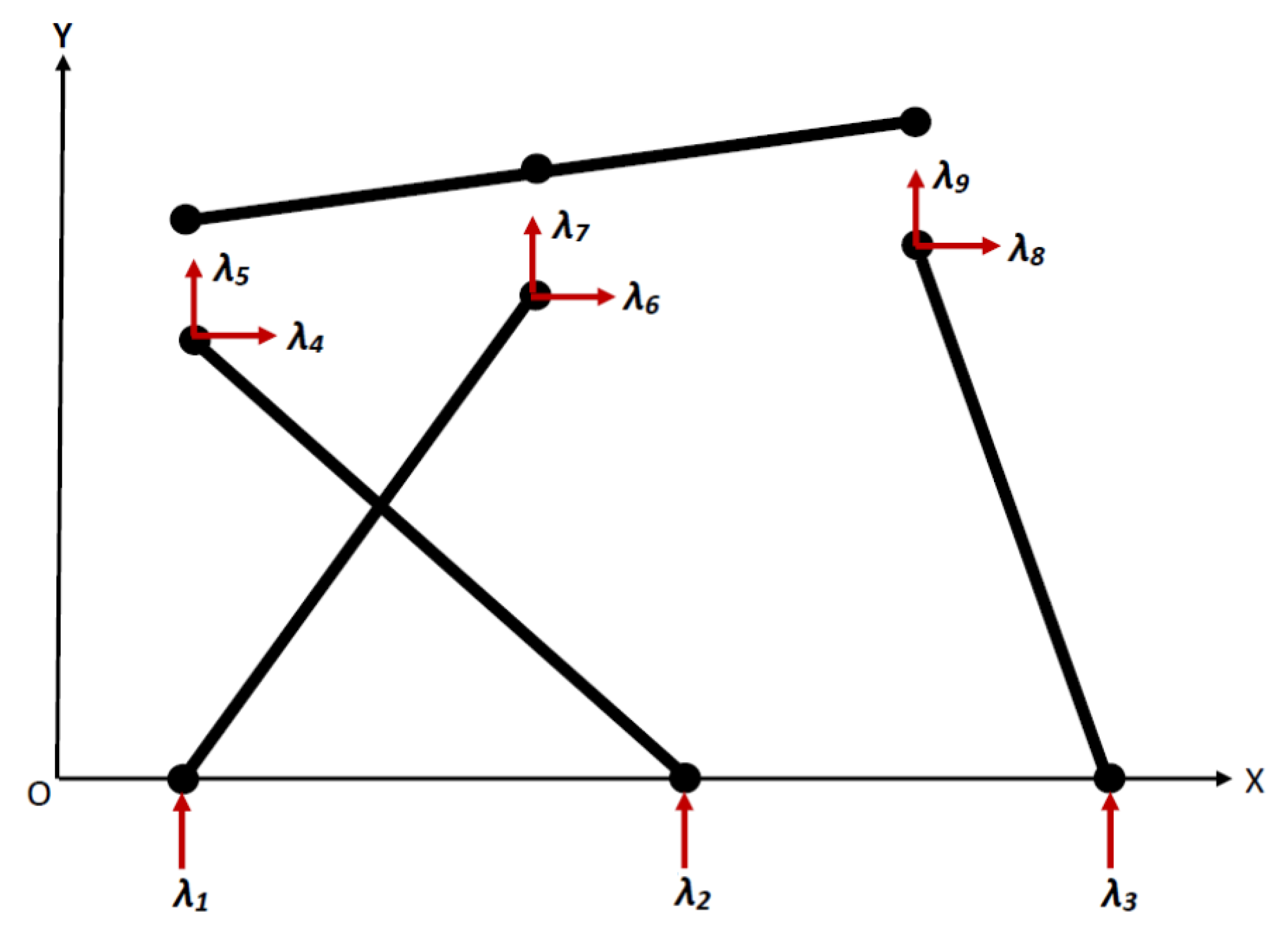
Among the nine Lagrange multipliers in Equation (18), six multipliers correspond to the internal reaction forces in x- and y-directions at the three upper joints of the mechanism, whereas the other three multipliers correspond to the reaction forces at the three lower joints. These reaction forces are shown in Figure 3. Since the lower joints are prismatic joints with only one degree of freedom, i.e., translation in the x-direction, the reaction forces are exerted only in the y-direction, i.e., normal to the guideway of the sliders.
Hence, there is one reaction force required to be evaluated at every lower joint, which means there are three reaction forces at all the lower joints. The generalized joint reaction forces R, which include two reaction forces in the x- and y-directions at every upper revolute joint and one reaction force in the y-direction at every prismatic joint, are given by:
From Equation (22), it is understood that the joint reaction forces are dependent on the Jacobian of the mechanism B(q,t)T, which represents the change of the mechanism’s posture.
2.2. Friction Modeling
Since the friction forces cannot be derived from the energy expressions, their contribution to the dynamics is presented separately here. Although the friction can be modeled as being either linear or nonlinear and either symmetric or asymmetric, it is commonly modeled as symmetric and linear. Furthermore, the friction at the prismatic joints is typically much higher than that at the revolute joints. This is particularly true when roller or ball bearings are used as the revolute joints since the friction in such bearings is very small. Therefore, when the friction should be considered, one can either consider the friction at all of the joints or the friction at only the prismatic joints, while neglecting the friction at the revolute joints. The mechanism at hand uses roller bearings as the revolute joints. As a result, the friction at the revolute joints is not significant and therefore neglected.
In this work, the Stribeck friction model, as shown in Figure 4b, is used. This friction model is modified from the static-viscous-Coulomb friction model shown in Figure 4a by adding the Stribeck friction effect to the static, Coulomb, and viscous friction components. This can be written as:
where fs, fc, and fv denote diagonal matrices containing the static, Coulomb, and viscous friction parameters, respectively. For the case of a nonzero velocity in Equation (23), the first and the third terms in the right-hand side are the Coulomb and viscous friction components, whereas the second term is the Stribeck-effect friction component. Furthermore, some values of δ have been recommended. In this work, the value of 1 was used. Using this friction model, there are four friction parameters to be identified: fs, fc, fv, and vs. In the case of varying normal forces, the static and Coulomb friction forces vary accordingly. As a result, the static and Coulomb friction cannot be identified as forces in the usual manner. In such a case, which is the case in this work, the static and Coulomb frictions should be identified as coefficients, i.e., μs and μc.
The static and Coulomb friction parameters in the case of a translational joint, i.e., prismatic joint, are given by multiplying each of a dimensionless static friction coefficient μs and a dimensionless Coulomb friction coefficient μc by the normal force fn exerted on the contact surface at the joint:
The static and Coulomb friction coefficients typically depend on the types of materials in contact with each other and the lubrication condition.
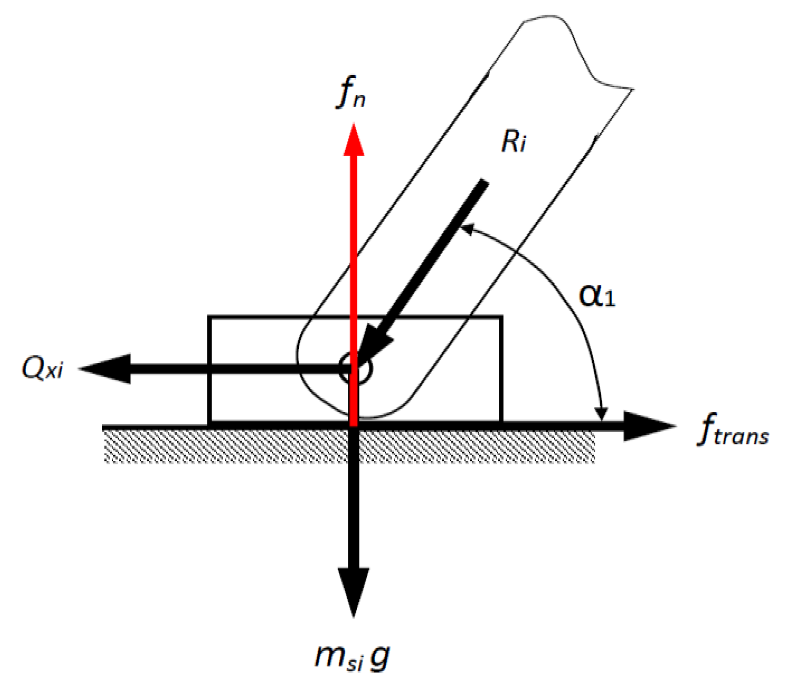
In general, the normal force in a posture-changing mechanism, such as a PKM like the mechanism at hand, is not constant. In the prismatic joint of the mechanism at hand, as illustrated in Figure 5, three force components are acting, namely, the weight of the prismatic joint msig, which is given by the total weight of the slider and the moving part of the linear motor; the input force Qxi exerted on the prismatic joint by the linear motor; and the force Ri exerted to the prismatic joint due to the weight of the other components mounted on the slider, as well as the external payload and the external force, if any. The exerted force Ri can be decomposed into horizontal and vertical components, namely, Rxi and Ryi. At any time, the total force in the horizontal direction is given by the sum of Rxi and Qxi. In a static case, Rxi is overcome by Qxi such that the total force in the horizontal direction is zero. However, when the prismatic joint is in motion, the magnitude of Qxi is different from the magnitude of Rxi. If the magnitude of Rxi is larger, the slider is moving toward the equilibrium state of the mechanism, i.e., the mechanism is collapsing to the base in the case of mechanism working in XY plane. Conversely, if the magnitude of Qxi is larger, this means that the slider is moving due to an actuation point.
The normal force fn is equal but in the opposite direction to the sum of all the vertical force components. This can be written as follows:
Although the weight of the prismatic joint, i.e., the first term on the right-hand side of Equation (25), is constant, the force component Ryi varies in general, depending on the mechanism posture. As a result, the normal force fn, and accordingly the static and Coulomb friction parameters, fs and fc, are not constant.
Since the varying components of the normal forces are mainly due to the effect of gravity and the external force, the posture dependency of the static and Coulomb friction parameters as described above is more significant when the rigid body motion of the mechanism is against a gravitational load, i.e., the rigid body motion is in the XY plane and/or under an external force. However, when the mechanism is free from an external force and working in the XY plane while it is statically balanced by a gravitational compensation mechanism or the mechanism is working in XZ plane, i.e., horizontally, then the posture dependency is less significant. The external force can be excluded during the dynamic parameter identification by simply moving the mechanism without any working load. In such a case, only the gravitational effect remains, if any. When the mechanism working in the XY plane is statically balanced, the gravity effect is eliminated.
When the mechanism is working in the XZ plane, the gravitational effect is working in the off-plane direction and most of the weight of all the mechanism components is borne by the structure of the mechanism. This does not mean that the gravitational effect is eliminated from the joints. In fact, the prismatic and revolute joints are still subject to the gravity-induced load but it works in the off-plane direction. At the prismatic joint, this gravity-induced load can be seen as a vertical reaction force that is exerted on the base of a cantilever due to the weight of the cantilever. In addition to this vertical reaction force, there are also a horizontal reaction force and a reaction moment at the prismatic joint due to the weight of the cantilever. If the external force is excluded, the vertical reaction force will be the main force component, which results in an off-plane normal force working at the prismatic joint. In addition to this normal force component, there is also an in-plane normal force component that results from the motion of the mechanism. All of these normal forces lead to a friction force, which should be overcome during the actuation of the mechanism. Similarly, the off-plane normal forces that are equal but in the opposite direction to the bearing thrust forces also arise in the revolute joints. In addition to this, there are also in-plane normal forces at the revolute joints resulting from the motion of the mechanism. Furthermore, if an in-plane external force exists, it will be additionally exerted to the prismatic and revolute joints. If the external force does not have a varying vertical (off-plane) component, the vertical (off-plane) normal forces working at the three prismatic and revolute joints may be assumed to be uniform. Accordingly, the static and Coulomb friction parameters may be assumed to be constant. A more detailed friction formulation for the mechanism working in the XZ plane can be seen in Section 5.
2.3. Dynamic Model with Friction
By incorporating the friction forces, the equations of motion in Equation (14) can be expanded to the following:
The differential-algebraic equations in Equation (16) then become:
The partitioned differential-algebraic equations are accordingly given by:
The inverse dynamics can still be presented in the compact expression given in Equation (19), but the vector should be modified to the following:
It is worth mentioning that the friction forces can only be evaluated after the corresponding normal forces are evaluated, whereas the normal forces can only be computed after the corresponding Lagrange multipliers are computed. In fact, the Lagrange multipliers are not available at the initial time. For this reason, a statics formulation of the mechanism is used at the initial time to compute the normal forces. This is valid since the mechanism is at rest at the initial time. The detailed statics formulation used to obtain the static normal forces is not presented here to reduce the paper’s length. In short, the static equations can be written based on the static equilibrium principle, and subsequently, can be presented as a linear system that can be solved for the normal forces, i.e., the reaction forces, by inverting the linear system.
3. Identification Algorithm
The mathematical model function Y, which serves as the base of the nonlinear identification, such as in the case of this work, is given directly by the nonlinear inverse dynamics model of the system, i.e.:
The residual error of the estimation is given by the difference between the estimated active joint forces and the measured active joint forces :
where the estimated active joint forces are defined similarly to Equation (30) but using the estimated parameters instead:
An identification algorithm is defined to minimize the residual error in Equation (31). This is most commonly achieved by minimizing a cost function given by the square of the residual error, i.e.:
The dynamic parameter identification can be stated as the following optimization problem: find the estimates of the dynamic parameters that minimize the cost function J defined in Equation (33).
A bound-constrained optimization method was applied in this work to minimize the residual error. An iterative bound-constrained global optimization solver in MATLAB® R2020a, namely, a constrained pattern search [16,17] was applied. The global search tool was used instead of a local search tool to avoid getting trapped in local minima.
To ensure that the estimates are physically feasible, some physical feasibility constraints should be incorporated into the estimation algorithm. This changes the least squares problem into a constrained optimization problem as follows: minimize the residual error, which is commonly represented by the square of the residual error, subject to the physical feasibility constraints. In this work, the physical feasibility is imposed by predefining bounds of the estimates in the estimation algorithm. Since the bound constraints are used as the physical feasibility constraints, the estimation problem can be written as:
where LB and UB denote the lower and upper bounds, respectively. The bounds are introduced to narrow the search space and avoid getting trapped at unexpected local minima.
This approach requires a priori knowledge of the numerical values of the estimated parameters. This can typically be obtained by using CAD data, manufacturer’s data, or direct measurements of the main components. In general, this a priori data is not accurate, and therefore some lower and upper bounds are determined to capture the expected true values of the parameters. In this case, one should provide acceptable bounds, which will ensure the physical feasibility but one should not provide bounds that are too tight as they may fall beyond the true values of the parameters. Moreover, the span from the a priori values to the lower bounds does not need to be equal to that from the a priori values to the upper bounds; the spans depend on how much the tendency of the true values to be shifted down or up from the a priori values. The true value of a mass, for example, tends to be shifted up from the a priori value rather than shifted down due to additional components or accessories mounted on the main components, such as fasteners, cables, etc.
This approach is used since the design or nominal values of the parameters in this work can be obtained easily for some reasons: the masses of the components are known and the CAD models of the components are available. The masses of the components can be obtained by weighing them or calculating them from the volume and the material density of the components. The earlier is more practical when it is possible to disassemble the components and weigh them, whereas the latter can be done if weighing is not possible. The determination of the COM positions of the components in this work was simplified to one dimension as the geometry of the components was symmetric in the other two dimensions. These COM positions could be easily obtained using CAD software, which is PTC Creo Parametric 4.0 in this work, since the CAD models are available. Once the masses and the COM positions of the components are known, the first moments and the moments of inertia of the components can be easily calculated.
4. Optimal Exciting Trajectory
In the dynamic parameter identification, the exciting trajectory should be optimized to persistently excite the dynamics of the mechanism. For convenience, either a polynomial or sinusoidal exciting trajectory is typically used. Since the latter is periodic and can in general generate more complicated trajectories, it was used in this work. This trajectory is parameterized by using the following Fourier series:
where and f are the harmonic number and the fundamental frequency in Hz, respectively, whereas the subscript i corresponds to the ith generalized coordinate q. The parameters and f should be predefined. For the mechanism at hand, i = 1, 2, 3, where q1, q2, and q3 are given by the coordinates of the end-effector, i.e., x, y, and θ.
It can be observed in Equation (35) that the parameters that should be determined for an optimized exciting trajectory are qi0, aij, and bij. The total number of these parameters is:
The optimization of the exciting trajectory is performed to optimize an objective function, which indicates the rank of the system subject to some constraints of the mechanism. The constraints used are typically the reachable workspace; collision avoidance; and the limits of the position, velocity, acceleration, and forces of the active joints, zero initial and final velocity, and zero initial and final acceleration. Since the parameterized exciting trajectory is expressed in terms of the new parameters qi0, aij, and bij, the objective function G should also be expressed in terms of these new parameters. In this work, the exciting trajectory optimization could be stated as the following constrained optimization problem: find that optimize the objective function G subject to:
The objective function G used in this work was a weighted composite of the condition number and inverse of the minimum singular value of the observation matrix W in the linear form of the inverse dynamics equations with respect to the dynamic parameters [13], i.e.:
where w1 and w2 denote the corresponding weights.
5. Experimental Results and Discussions
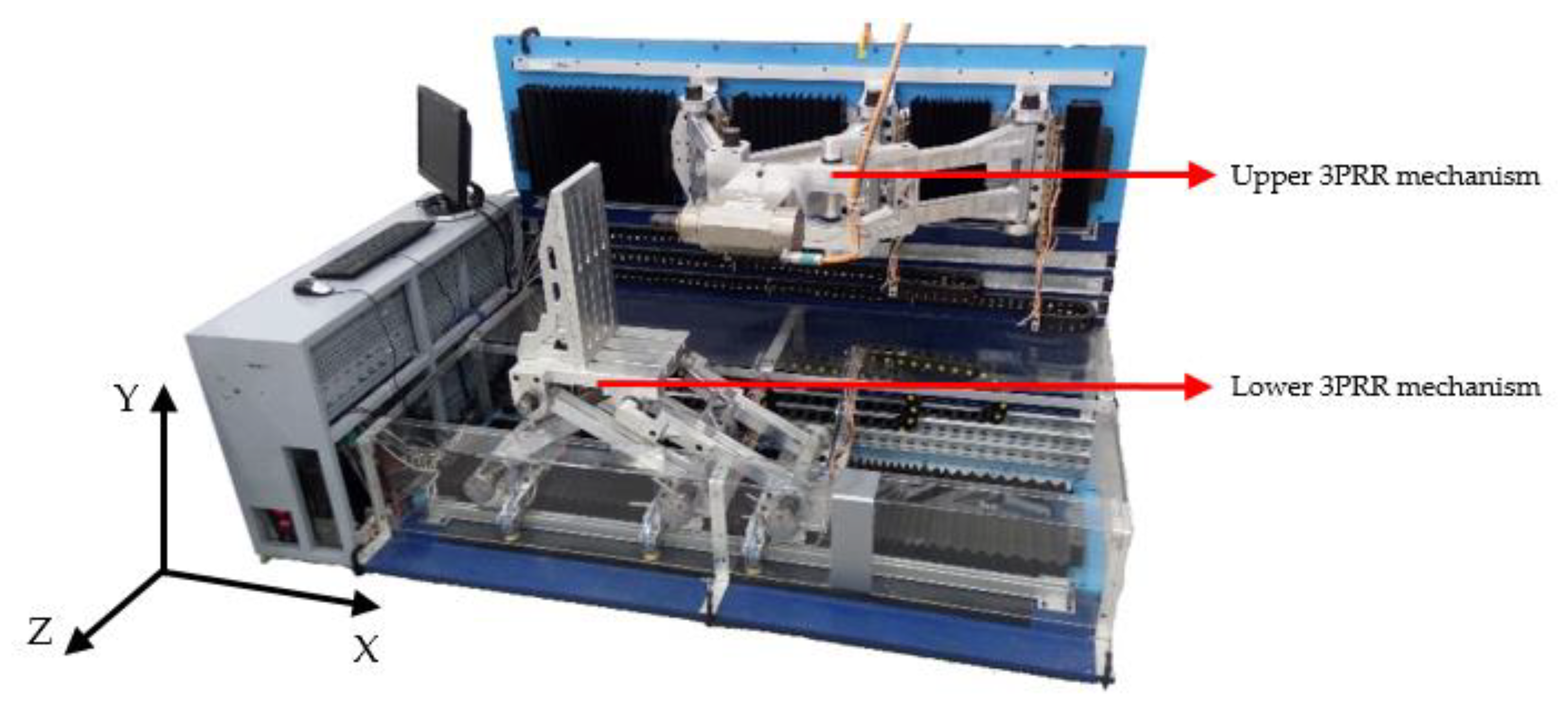
The upper mechanism of a hybrid-kinematics machine shown in Figure 6 was used in the experiment. This 3PRR mechanism has legs with lengths of L1 = 600 mm, L2 = 475 mm, and L3 = 604 mm. The position of the upper revolute joints on the moving platform was given by xp2 = xp3 = 280 mm. The COMs of the legs were L1G = 240.1 mm, L2G = 207.1 mm, and L3G = 272.8 mm, whereas the COM of the moving platform was xPG = 239.5 mm. In this experiment, the upper mechanism was oriented horizontally, i.e., in the XZ plane, and therefore its rigid body motion was not affected much by gravity, as discussed earlier.
5.1. Optimization Setup
A bound-constrained optimization using MATLAB pattern search with a GPS Positive basis 2N poll method and default stopping criteria was implemented to estimate the dynamic parameters of the mechanism based on the nonlinear form of the inverse dynamics model with a varying nonlinear Stribeck friction model. For simplicity, the masses of the three sliders were assumed to be identical and the friction on the three prismatic joints was assumed to be uniform. Therefore, there was only a single value of each friction parameter instead of three values corresponding to the three sliders. Aside from simplicity concerns, this assumption was justified because all of the sliders moved on the same guideway.
The iterative optimization algorithm was executed by using the design values as the initial values. Table 1 shows the available design values of the inertial parameters, along with the determined bounds. The bounds of the inertial parameters were determined to be wider toward the upper limits since it was expected that the actual values of the parameters were larger than the design values due to additional parts being attached to the main components. On the other hand, wide non-negativity bounds from zero to infinity were applied to the friction parameters since there was no a priori information on their expected values.
5.2. Friction and Input Forces
Since the mechanism was oriented horizontally, the friction at the prismatic joints, i.e., between the sliders and the guideway, could be decomposed into two main components: the friction component due to the normal forces in the y-direction and the friction component due to the normal force in the z-direction. The former normal forces fn,yi were exerted vertically on the prismatic joints due to the weight of the mechanism:
The parameter αi represents the portion of the moving platform weight that was supported by the slider i. The sum of all values of αi should be 1. The best constant value of αi was obtained by attempting various values. After some attempts, the obtained best values for i = 1, 2, 3 were 0.7, 0.2, and 0.1, respectively. For simplicity, the friction forces corresponding to these normal forces, i.e., the normal forces in the y-direction, were assumed to be constant and modeled using the static friction at the beginning of the motion and using Coulomb and viscous friction for the subsequent motion:
The latter normal forces, i.e., the normal force in the z-direction, act horizontally and vary with changes in the mechanism’s posture. These varying normal forces result in varying static and Coulomb friction forces. Since the static and Coulomb components of the friction were varying, the overall friction corresponding to the horizontal normal forces was varying.
Furthermore, the friction forces due to the normal forces in the y-direction needed to be added to Equation (19) when evaluating the input forces. Thus the input forces could be written as follows:
5.3. Data Acquisition and Filtering
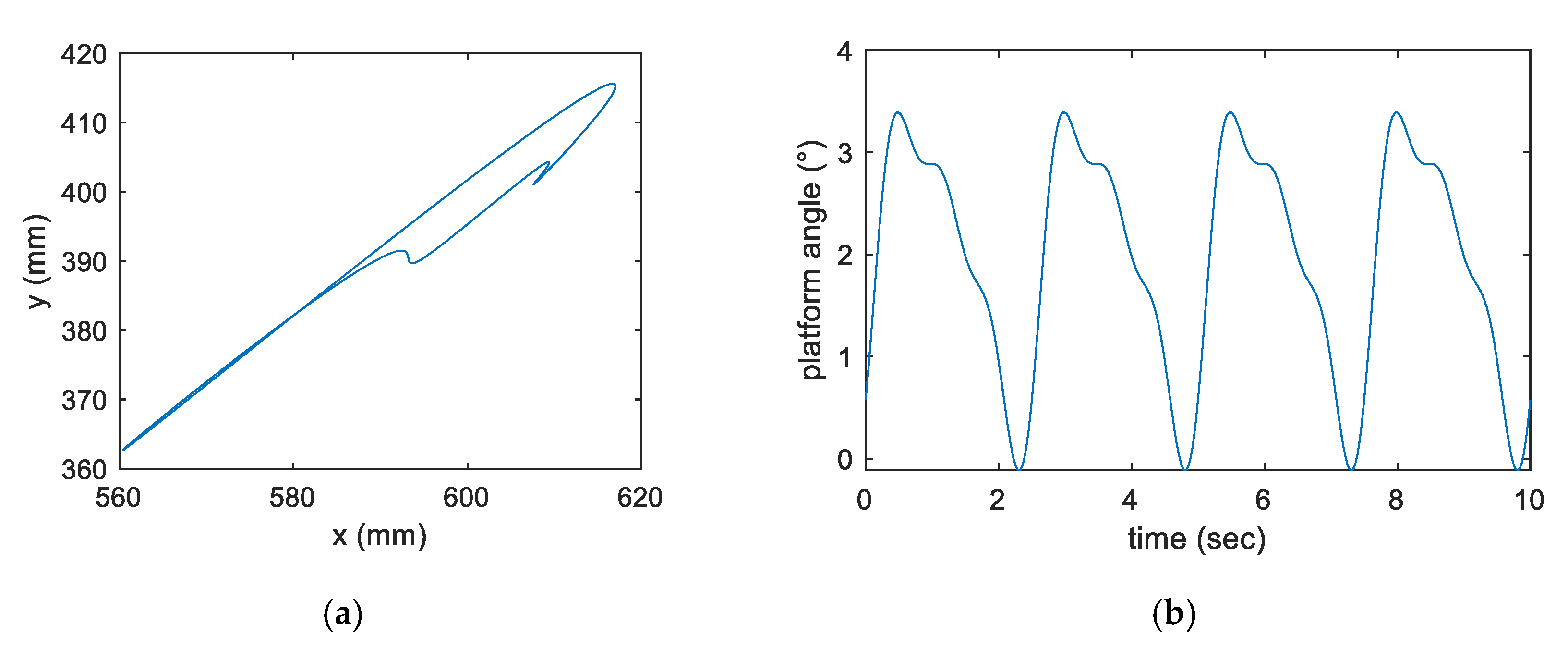
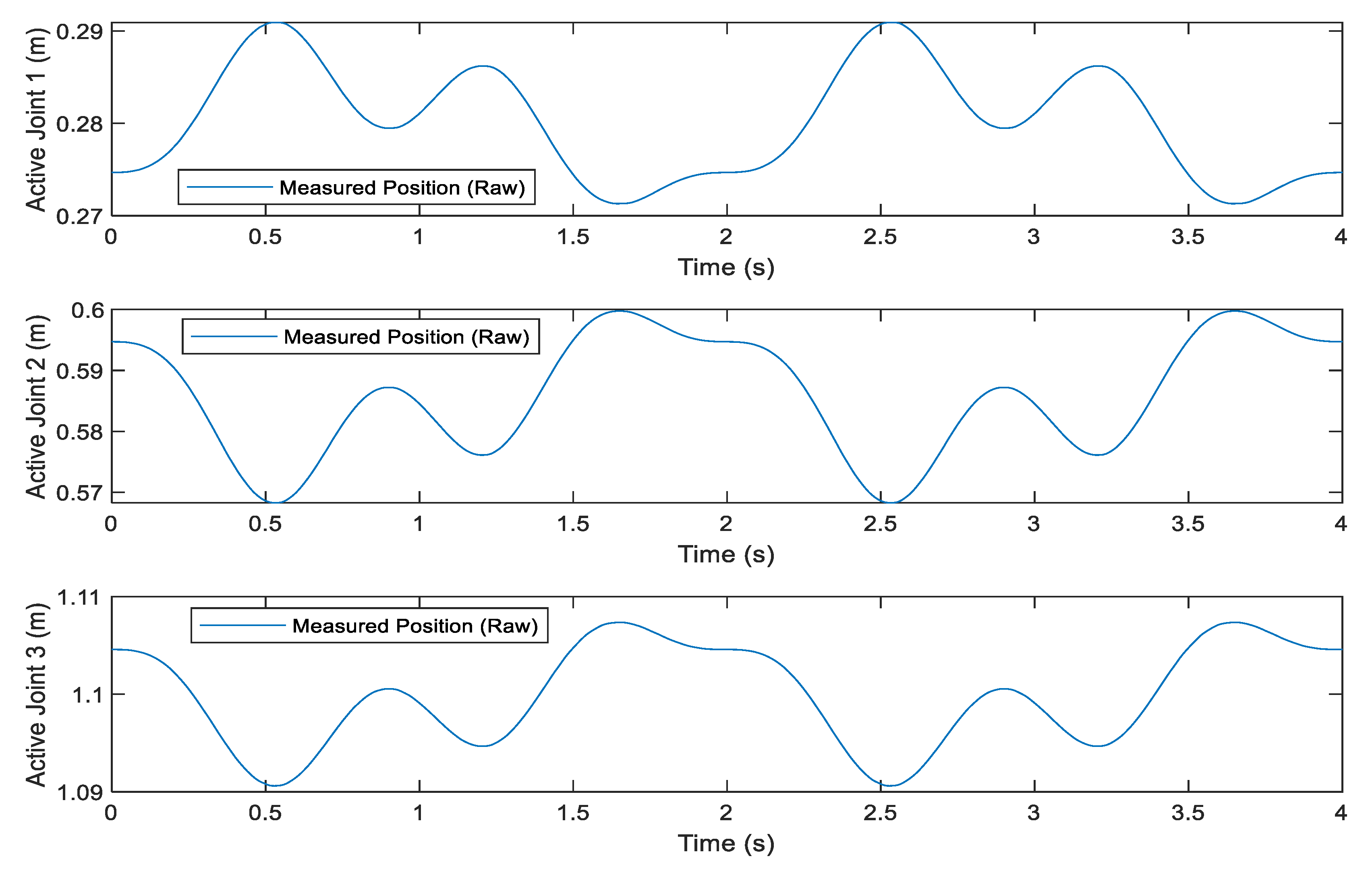
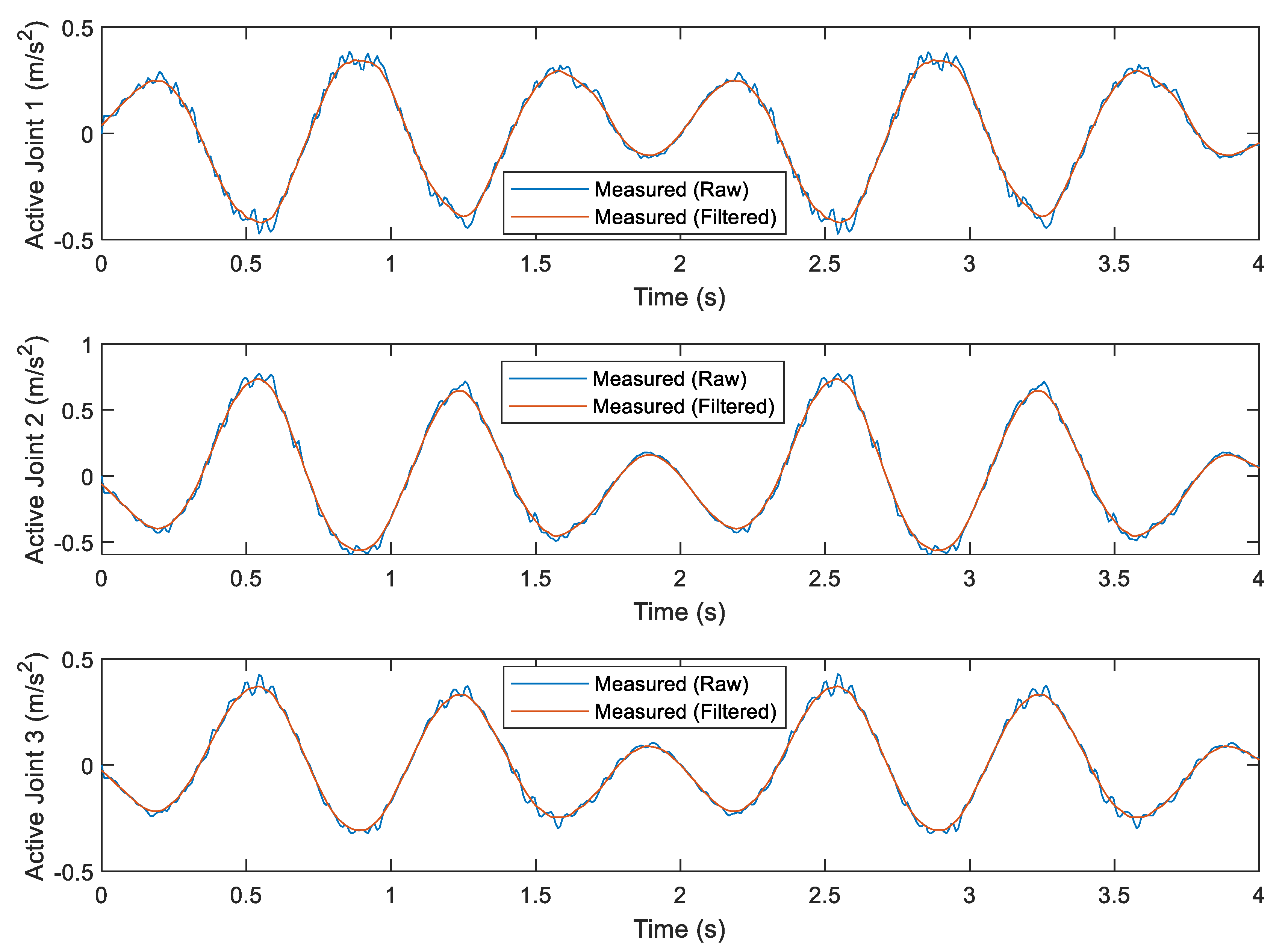
The sinusoidal trajectory given by Equation (35) and shown in Figure 7 was used as the optimal exciting trajectory of the end effector. Its parameters were obtained by optimizing Equation (38) subject to Equation (37). The definition of the optimized exciting trajectory included the position, velocity, and acceleration of the end effector within a defined timespan (4 s). Using the inverse kinematics, the motion variables of the trajectories defined in the task space were transformed into the active joint space. While the active joints were moving to make the trajectories, their motion variables were measured using linear encoders. The active joint positions were directly measured by using the encoders. The uncertainty of the encoders was ±0.0005 mm. The active joint velocities and accelerations were derived from the measured positions. The measured positions, velocities, and accelerations of the active joints are shown in Figure 8, Figure 9 and Figure 10, respectively. It is shown that the measured active joint positions were so smooth that they did not need any filtering. However, some noise was found in the measured velocities and accelerations. Therefore, they were filtered, as shown in Figure 9 and Figure 10. It should be noticed that the measured trajectory positions, velocities, and accelerations were used in the identification instead of the planned (commanded) ones.
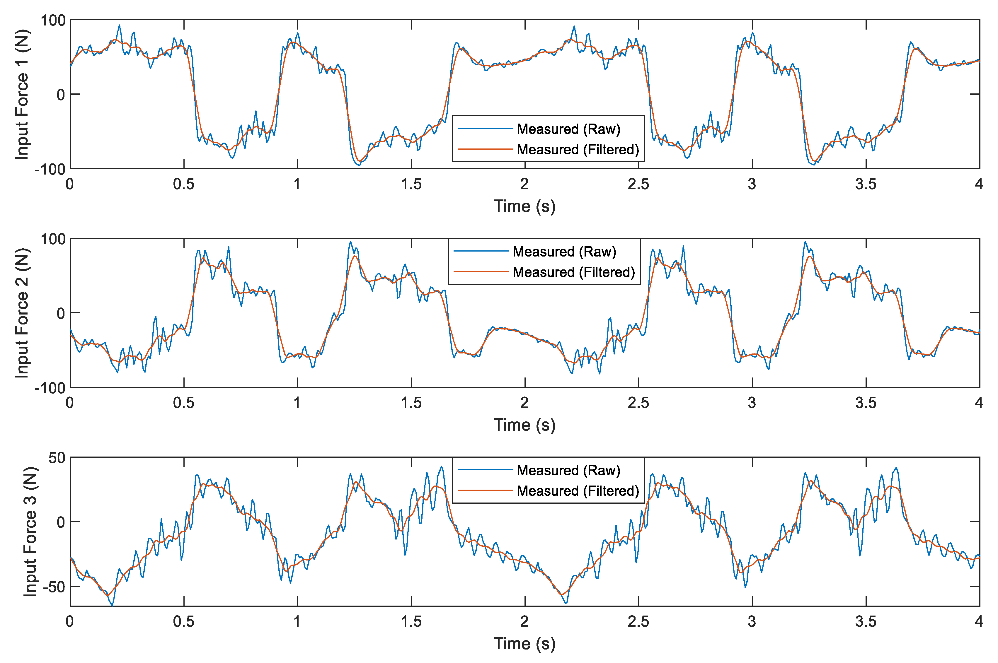
At the same time, the active joint forces were also measured. The active joint forces were not directly measured by using dedicated force sensors attached to the sliders. Instead, the measurement of the active joint forces was based on the voltage output from the controller to the servo drives. The active joint forces were calculated based on a proportional relationship between the voltage output from the controller to the servo drives and the resulting current in the servo drives, as well as a proportional relationship between the current drawn from the servo drives and the resulting actuation forces. This indirect measurement of the active joint forces was much cheaper than a direct measurement as no dedicated force sensors were required. The uncertainty of the active joint force measurement was ±0.0381 N. The measured active joint forces are shown in Figure 11. As the measured active joint forces were noisy, they were filtered, as shown in Figure 11. The filtering of the velocities, accelerations, and forces were all performed by using a Savitzky–Golay smoothing filter in MATLAB. Thus, all the raw data were acquired from the hardware and subsequently filtered in MATLAB using the aforementioned filter.
5.4. Results
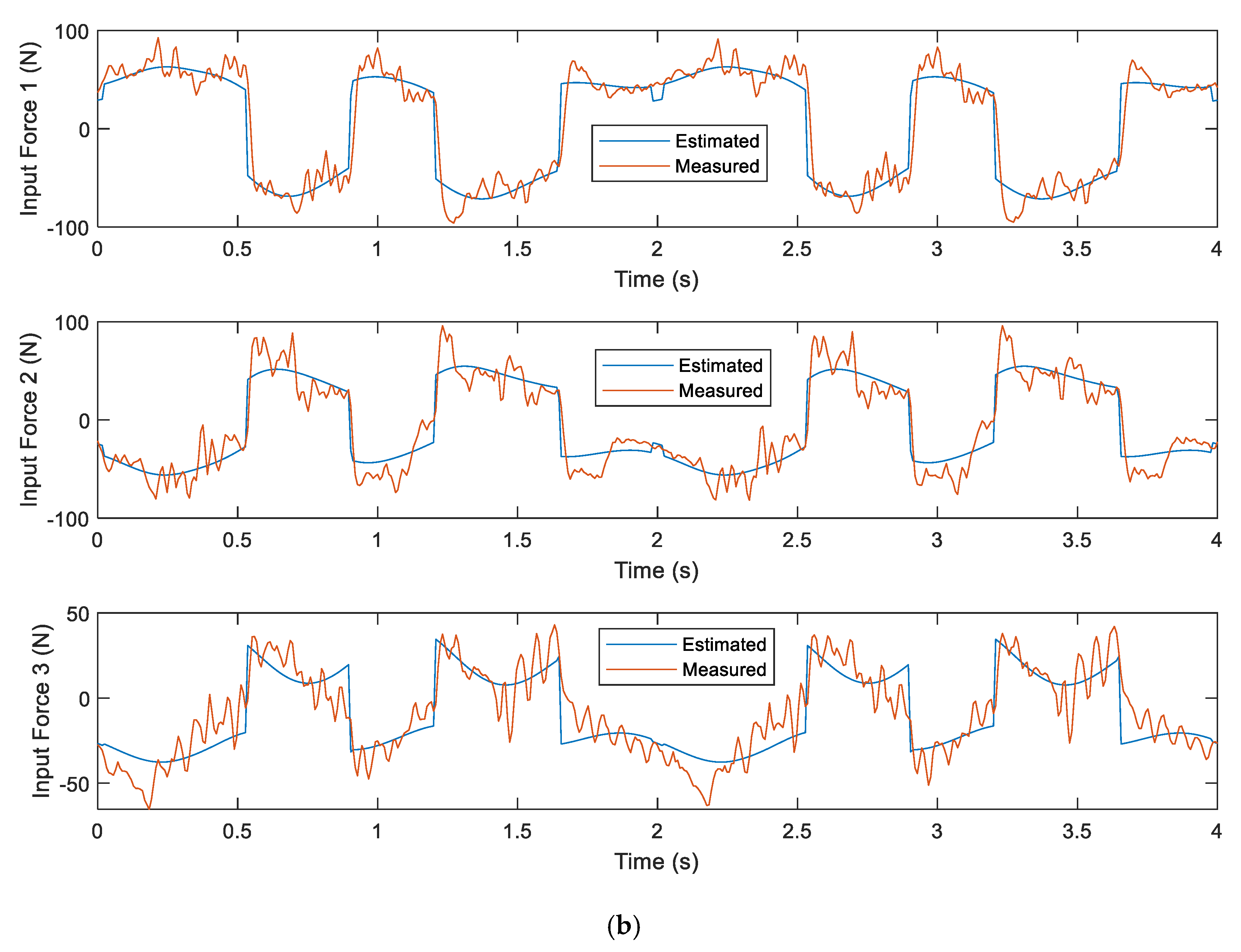
In the following presentation of results, the estimated input forces are plotted together with the raw, measured input forces, not the filtered ones, for a more genuine comparison, although the identification used the filtered, measured input forces. Table 1 shows the estimates of the dynamic parameters, which consisted of the barycentric inertial parameters and the friction parameters. It can be seen that the estimated inertial parameters were larger than their design values. This was expected since the actual masses should be larger than their design values due to the attached additional parts, such as the nuts, cables, etc. The plots of the estimated and measured input forces created using the Coulomb-viscous friction and Stribeck friction models are shown in Figure 12a,b, respectively. It is shown that the latter friction model provided a better fit, whereas the former friction model was not adequate to represent the real dynamics. This justified the use of the Stribeck friction model instead of the Coulomb-viscous friction model.
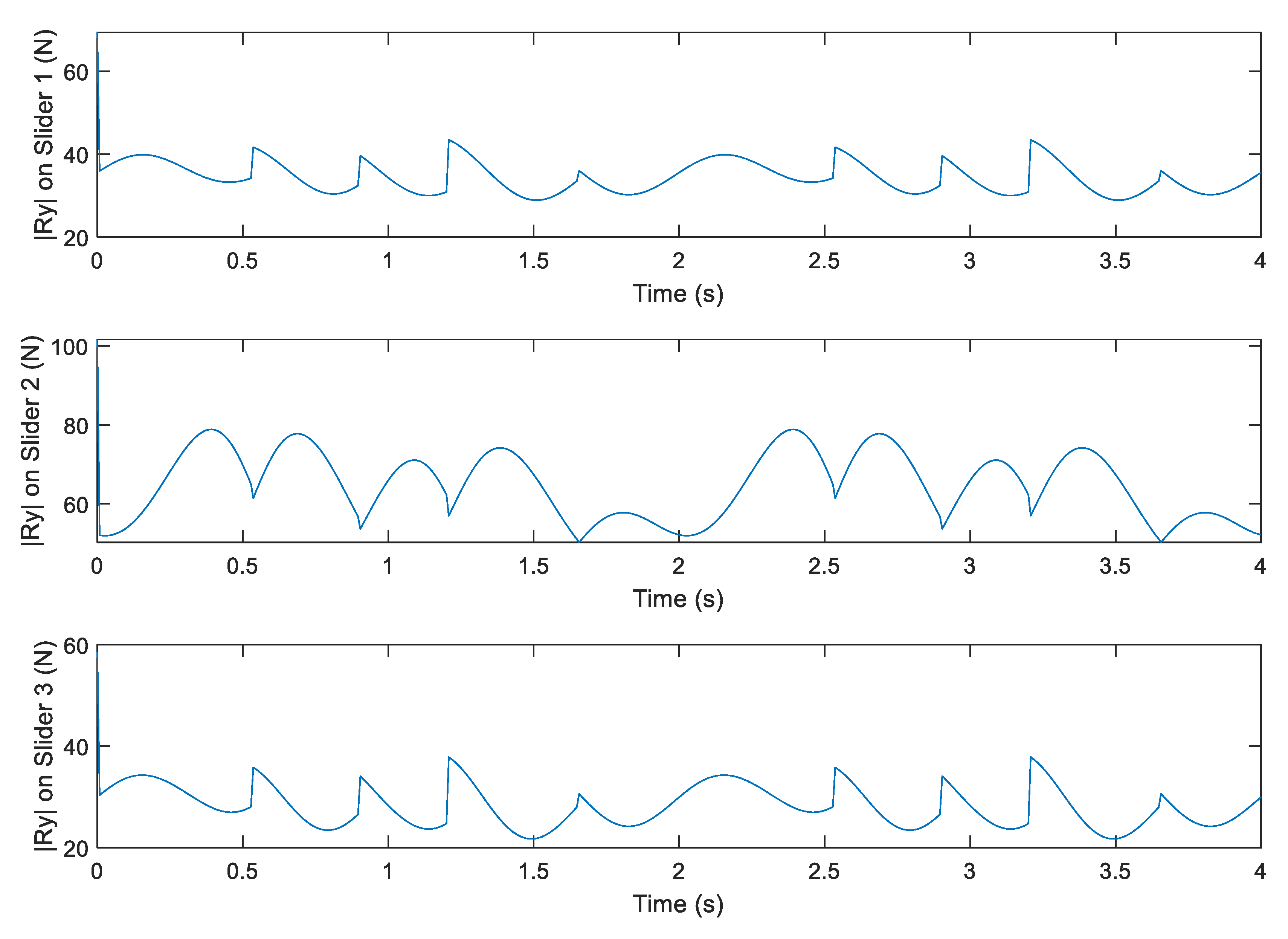
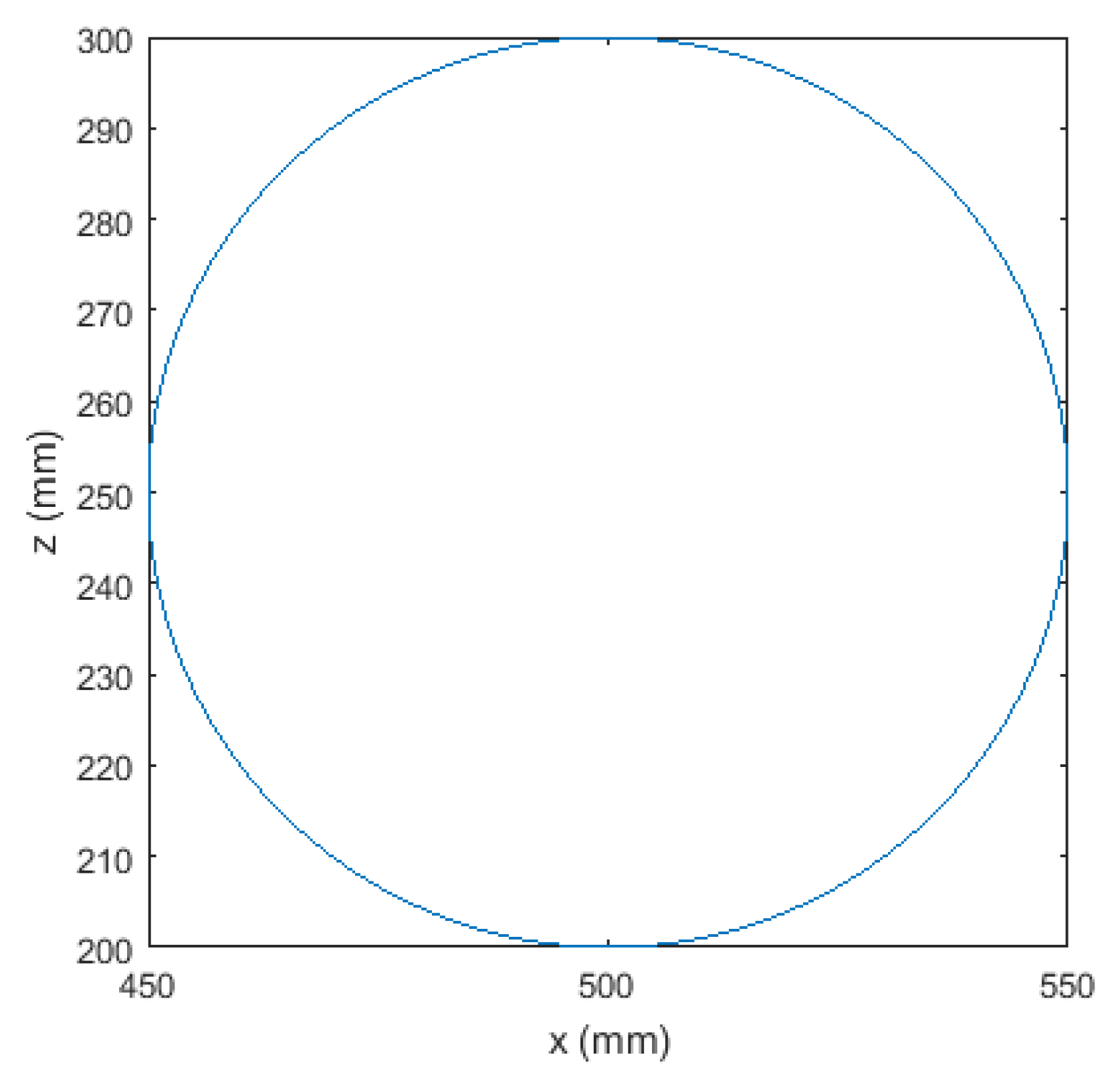
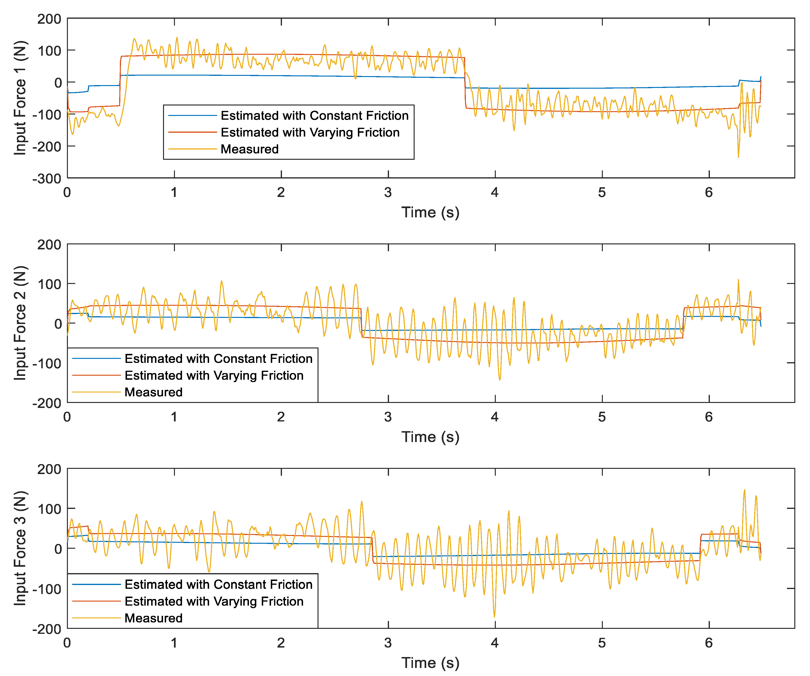
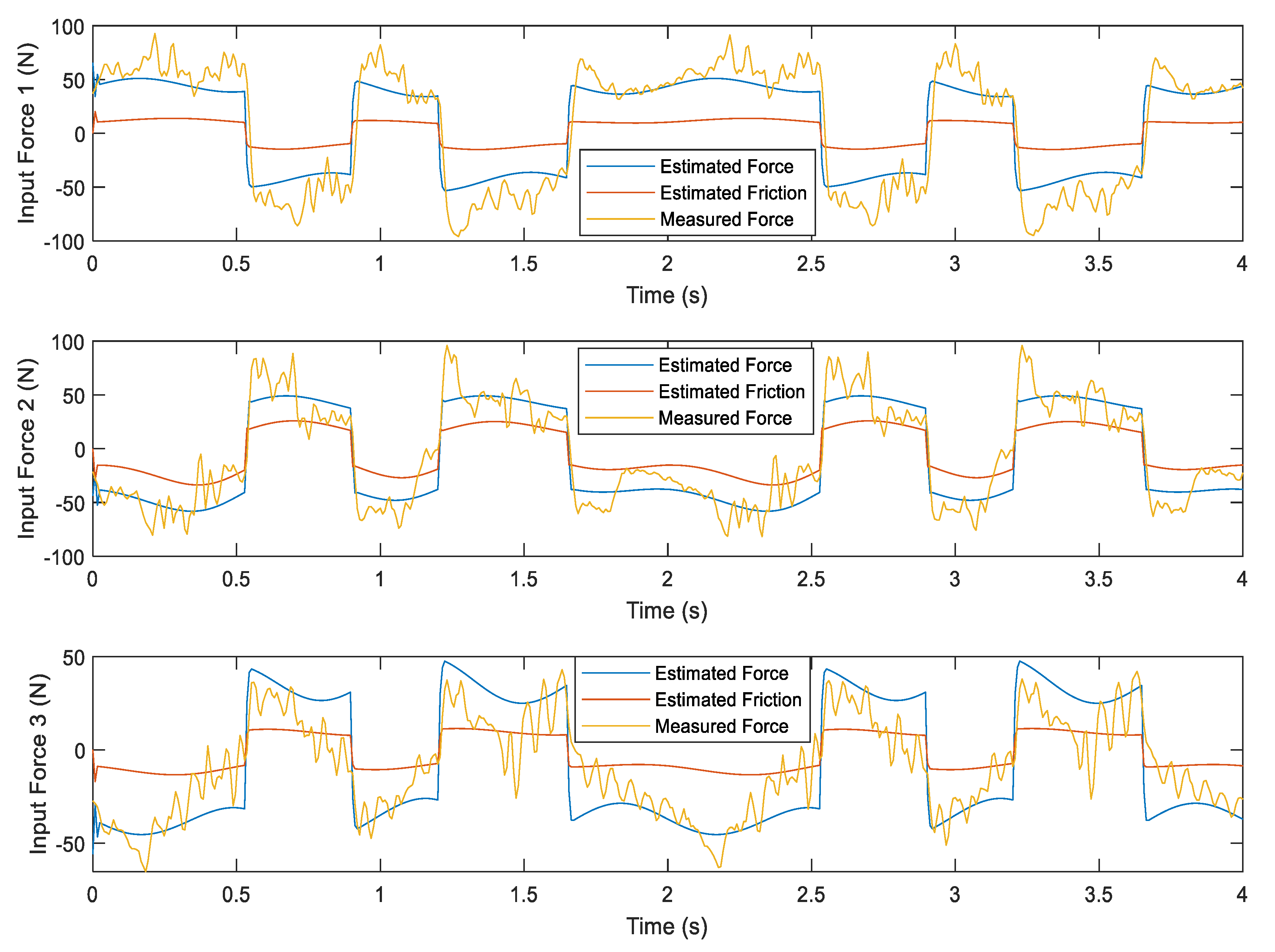
The variation of the absolute values of the vertical reaction forces Ry on the three prismatic joints is shown in Figure 13. The absolute values are plotted here instead of the signed values to show the variation of the values more clearly. The variation of these normal forces resulted in the variation of the friction forces. The solution obtained by considering the varying friction, as shown in Table 1, was validated by applying some other exciting trajectories that were different from the one used in the identification. Figure 14 shows a full-circle trajectory executed for the validation, while Figure 15 shows the corresponding estimated and measured input forces. It is shown that the input forces estimated by considering the varying friction forces had a better fit than the input forces estimated by considering constant friction forces. Finally, Figure 16 shows the plots of the estimated input forces along with the estimated friction forces. The figure clearly shows the contribution of the significant friction to the overall dynamics.
6. Conclusions
It was shown that the iterative bound-constrained optimization method provided physically feasible estimates in the dynamic parameter identification with noisy measurements. The predefined bounds of the parameters were used as the constraints to ensure the physical feasibility of the solutions. These bounds can be obtained based on any a priori knowledge of the system, such as the design values obtained from a CAD model or the measurement data of the individual main components before the assembly. In a PKM with sliding joints, it was shown that the friction on the slider guideway was significant and therefore could not be neglected. Furthermore, the Stribeck friction model was shown to more accurately represent the friction and therefore provide a better dynamic model. In this work, the variation of the normal forces, which resulted in the variation of the static and Coulomb friction forces, were taken into consideration in the dynamic modeling and dynamic parameter identification of the PKM. This variation, unless it is negligible, should always be taken into consideration when dealing with PKMs since this variation is an inherent characteristic of the PKMs due to the changing posture of the mechanism. As a consequence of considering the variation of the static and Coulomb friction forces, which was the main contribution of this work, the static and Coulomb friction parameters fs and fc could not be identified as constant parameters since they were varying. Instead, the static and Coulomb friction coefficients µs and µc were identified since they were constant parameters. The product between these coefficients and the varying normal forces gives the varying static and Coulomb friction parameters fs and fc.
Author Contributions
Both authors discussed the idea of this work and made scientific contributions. A.R. performed the work and wrote the paper. B.E.-K. guided the work, gave advice, and reviewed the paper. Both authors have read and agreed to the published version of the manuscript.
Funding
This publication was based upon work supported by the Khalifa University of Science and Technology under Award No. RC1-2018-KUCARS.
Conflicts of Interest
The authors declare no conflict of interest.
References
- Hoang, N.-B.; Kang, H.-J. Observer-based Dynamic Parameter Identification for Wheeled Mobile Robots. Int. J. Precis. Eng. Manuf. 2015, 16, 1085–1093. [Google Scholar] [CrossRef]
- Farhat, N.; Mata, V.; Page, A.; Valero, F. Identification of dynamic parameters of a 3-DOF RPS parallel manipulator. Mech. Mach. Theory 2008, 43, 1–17. [Google Scholar] [CrossRef]
- Thanh, T.D.; Kotlarski, J.; Heimann, B.; Ortmaier, T. Dynamics identification of kinematically redundant parallel robots using the direct search method. Mech. Mach. Theory 2012, 52, 277–295. [Google Scholar] [CrossRef]
- Poignet, P.; Ramdani, N.; Vivas, O.A. Robust estimation of parallel robot dynamic parameters with interval analysis. In Proceedings of the 42nd IEEE International Conference on Decision and Control, Maui, HI, USA, 9–12 December 2003. IEEE Cat. No.03CH37475. [Google Scholar]
- Pan, Y.-R.; Shih, Y.-T.; Horng, R.-H.; Lee, A.-C. Advanced Parameter Identification for a Linear-Motor-Driven Motion System Using Disturbance Observer. Int. J. Precis. Eng. Manuf. 2009, 10, 35–47. [Google Scholar] [CrossRef]
- Gautier, M.; Khalil, W.; Restrepo, P.P. Identification of the Dynamic Parameters of a Closed Loop Robot. In Proceedings of the IEEE International Conference on Robotics and Automation, Nagoya, Japan, 21–27 May 1995. [Google Scholar]
- Guegan, S.; Khalil, W.; Lemoine, P. Identification of the Dynamic Parameters of the Orthoglide. In Proceedings of the IEEE International Conference on Robotics and Automation—ICRA 2003, Taipei, Taiwan, 14–19 September 2003; pp. 3272–3277. [Google Scholar]
- Vivas, A.; Poignet, P.; Marquet, F.; Pierrot, F.; Gautier, M. Experimental dynamic identification of a fully parallel robot. In Proceedings of the IEEE International Conference on Robotics & Automation, Taipei, Taiwan, 14–19 September 2003. [Google Scholar]
- Renauda, P.; Vivas, A.; Andreff, N.; Poignet, P.; Martinet, P.; Pierrot, F.; Company, O. Kinematic and dynamic identification of parallel mechanisms. Control Eng. Pract. 2006, 14, 1099–1109. [Google Scholar] [CrossRef]
- Rodríguez, M.D.; Iriarte, X.; Mata, V.; Ros, J. On the Experiment Design for Direct Dynamic Parameter Identification of Parallel Robots. Adv. Robot. 2009, 23, 329–348. [Google Scholar] [CrossRef]
- Rodríguez, M.D.; Mata, V.; Valera, A.; Page, A. A methodology for dynamic parameters identification of 3-DOF parallel robots in terms of relevant parameters. Mech. Mach. Theory 2010, 45, 1337–1356. [Google Scholar] [CrossRef]
- Shang, W.; Cong, S.; Kong, F. Identification of dynamic and friction parameters of a parallel manipulator with actuation redundancy. Mechatronics 2010, 20, 192–200. [Google Scholar] [CrossRef]
- Briot, S.; Gautier, M. Global identification of joint drive gains and dynamic parameters of parallel robots. Multibody Syst. Dyn. 2015, 33, 3–26. [Google Scholar] [CrossRef] [Green Version]
- Rosyid, A.; El-Khasawneh, B.; Alazzam, A. Optimized Planar 3PRR Mechanism for 5 Degrees-Of-Freedom Hybrid Kinematics Manipulator. In Proceedings of the ASME 2015 International Mechanical Engineering Congress and Exposition IMECE2015, Houston, YX, USA, 13–19 November 2015. [Google Scholar]
- Rosyid, A.; El-Khasawneh, B.; Alazzam, A. Identification of lonely barycentric parameters of parallel kinematics mechanism with rank-deficient observation matrix. In Proceedings of the 11th International Symposium on Mechatronics and its Applications (ISMA), Sharjah, UAE, 4–6 March 2018. [Google Scholar]
- Kelley, C.T. Iterative Methods for Optimization; Society for Industrial and Applied Mathematics: Philadelphia, PA, USA, 1999; pp. 87–108. [Google Scholar]
- Audet, C.; Dennis, J.E., Jr. Analysis of Generalized Pattern Searches. SIAM J. Optim. 2003, 13, 889–903. [Google Scholar] [CrossRef] [Green Version]
Figure 1.
Planar 3PRR parallel kinematics mechanism (with the Z-axis perpendicular to the paper).

Figure 2.
Centers of masses (COMs) of a 3PRR parallel kinematics mechanism.

Figure 3.
Joint reaction forces corresponding to the Lagrange multipliers.

Figure 4.
(a) Static-viscous-Coulomb friction and (b) Stribeck friction models.

Figure 5.
Free-body diagram at the slider i, including the translational friction ftrans.

Figure 6.
Hybrid-kinematics machine composed of lower and upper 3PRR mechanisms.

Figure 7.
Exciting trajectory: (a) position and (b) angle.

Figure 8.
Raw measured active joint positions.

Figure 9.
Raw and filtered measured active joint velocities.

Figure 10.
Raw and filtered measured active joint accelerations.

Figure 11.
Raw and filtered measured input forces.

Figure 12.
Comparison between the estimated and measured input forces: (a) using the Coulomb-viscous friction model and (b) using the Stribeck friction model.
Figure 12.
Comparison between the estimated and measured input forces: (a) using the Coulomb-viscous friction model and (b) using the Stribeck friction model.


Figure 13.
Variation of the absolute values of the vertical reaction forces on the three prismatic joints during the identification motion.
Figure 13.
Variation of the absolute values of the vertical reaction forces on the three prismatic joints during the identification motion.

Figure 14.
Full-circle validation trajectory.

Figure 15.
Comparison between the estimated and measured input forces in the validation motion.

Figure 16.
Comparison between the estimated friction forces and the estimated input forces.


Table 1.
Estimates of the inertial and friction parameters using a nonlinear model with varying friction.
Table 1.
Estimates of the inertial and friction parameters using a nonlinear model with varying friction.
| Inertial Parameter | Lower Bound | Upper Bound | Design Value | Estimate | |
|---|---|---|---|---|---|
| msi | kg | 6.2550 | 9.3825 | 6.2550 | 7.2614 |
| mL1 | kg | 11.1280 | 16.6920 | 11.1280 | 12.1299 |
| mL2 | kg | 9.0800 | 13.6200 | 9.0800 | 10.0817 |
| mL3 | kg | 13.3720 | 20.0580 | 13.3720 | 14.4665 |
| mp | kg | 30.3510 | 45.5265 | 30.3510 | 31.3359 |
| mL1L1G | kg·m | 2.0039 | 4.0077 | 2.6718 | 3.3970 |
| mL2L2G | kg·m | 1.4104 | 2.8208 | 1.8805 | 2.4049 |
| mL3L3G | kg·m | 2.7355 | 5.4711 | 3.6474 | 3.6484 |
| mpxpG | kg·m | 5.4517 | 10.9035 | 7.2690 | 8.2238 |
| IL1 | kg·m2 | 0.7323 | 1.4648 | 0.9765 | 1.2206 |
| IL2 | kg·m2 | 0.4453 | 0.8906 | 0.5937 | 0.7421 |
| IL3 | kg·m2 | 1.0424 | 2.0847 | 1.3898 | 1.5088 |
| Ip | kg·m2 | 1.7989 | 3.5979 | 2.3986 | 2.9509 |
| Friction Parameter | |||||
| uc | - | 0 | ∞ | 0.1449 | |
| fv | Ns/m | 0 | ∞ | 83.1797 | |
| us | - | 0 | ∞ | 0.3016 | |
| vs | m/s | 0 | ∞ | 0.3281 | |
© 2020 by the authors. Licensee MDPI, Basel, Switzerland. This article is an open access article distributed under the terms and conditions of the Creative Commons Attribution (CC BY) license (http://creativecommons.org/licenses/by/4.0/).
Share and Cite
MDPI and ACS Style
Rosyid, A.; El-Khasawneh, B. Identification of the Dynamic Parameters of a Parallel Kinematics Mechanism with Prismatic Joints by Considering Varying Friction. Appl. Sci. 2020, 10, 4820. https://doi.org/10.3390/app10144820
AMA Style
Rosyid A, El-Khasawneh B. Identification of the Dynamic Parameters of a Parallel Kinematics Mechanism with Prismatic Joints by Considering Varying Friction. Applied Sciences. 2020; 10(14):4820. https://doi.org/10.3390/app10144820
Chicago/Turabian StyleRosyid, Abdur, and Bashar El-Khasawneh. 2020. "Identification of the Dynamic Parameters of a Parallel Kinematics Mechanism with Prismatic Joints by Considering Varying Friction" Applied Sciences 10, no. 14: 4820. https://doi.org/10.3390/app10144820
Note that from the first issue of 2016, this journal uses article numbers instead of page numbers. See further details here.