A Novel Deep Learning Approach for Tropical Cyclone Track Prediction Based on Auto-Encoder and Gated Recurrent Unit Networks

Abstract

Under global climate change, the frequency of typhoons and their strong wind, heavy rain, and storm surge increase, seriously threatening the life and property of human society. However, traditional tropical cyclone track prediction methods have difficulties in processing large amounts of complex data in terms of prediction efficiency and accuracy. Recently, deep learning methods have shown a potential capability to process complex data efficiently and accurately. In this paper, we propose a novel data-driven approach based on auto-encoder (AE) and gated recurrent unit (GRU) models to forecast tropical cyclone landing locations using the historical tropical cyclone tracks and various meteorological attributes. This approach fuses a data preprocessing layer, an AE layer, and a GRU layer with a customized batch process. The model is trained on a real-world tropical cyclone dataset from the years 1945–2017. Through a comparison with existing forecasting methods, the results verified that our proposed model performed around 15%, 42%, and 56% better than the Numerical Weather Prediction model (NWP) in 24, 48, and 72 h forecasts, and 27%, 13%, 17%, and 17% better than RNN, AE-RNN, GRU, and LSTM, respectively, in 24 h forecasts, using the absolute position error. In addition, a comparison of the meteorological variables indicated that the variable maximum sustained wind speed had the most significant effect on tropical cyclone track prediction.

1. Introduction

Tropical cyclones and typhoons are some of the extreme climate events that have a great impact on social and economic development, resulting in devastating natural disasters. Strong typhoons cause the loss of life and property, bringing catastrophic damage to coastal areas each year. For example, in 2017 alone, eight typhoons landed over China, affecting 5.879 million people and causing approximately five billion dollars in damage [1]. Therefore, it is important to predict the path of a tropical cyclone accurately so that governments and people can be better prepared for such a disaster. However, the formation of a tropical cyclone is affected by many factors, including the meteorological environment, thermodynamics, and kinetics of the tropical cyclone system. Moreover, there are also many factors that influence the path of a typhoon, including geostrophic deflection force, the location of the subtropical high pressure zone, the influence of cold air, and the topography of the inland areas [2]. The interplay of these factors makes forecasting tropical cyclone paths a significant challenge. Therefore, considering the impact of tropical cyclones on human beings and the complexity of their prediction, it is of great significance to research new tropical cyclone track forecasting methods.

Traditional prediction methods of tropical cyclone tracks are mainly statistical forecasting models and numerical prediction models [3]. Numerical models require a powerful computational capability to deal with complicated thermodynamic formulas and to simulate the internal structure of a tropical cyclone [4]. With the development of computer technology and the establishment of monitoring stations, the numerical model has been widely used, but it still has the problems of relatively high computational complexity and low prediction accuracy. For example, according to data published by the Shanghai Typhoon Institute, errors of approximately 97.4, 188.2, and 302.7 km have occurred in typhoon path prediction during 24, 48, and 72 h time windows when using a numerical model, whereas such errors were only approximately 84.2, 145.6, and 205.4 km when using a subjective empirical approach [5]. Statistical models for finding tropical cyclones based on characteristics from the historical records are unable to further improve the prediction accuracy [6]. Additionally, with the establishment of ocean observation stations, ground stations, and meteorological satellites, the volume of data available is also increasing, resulting in a big data problem to predict tropical cyclone paths. Deep learning algorithms have recently been applied to image processing, natural language processing, and object detection [7,8], showing significant strength in processing the large volume of complex data in two aspects. On one side, deep learning algorithms can conduct hidden feature extraction from a massive dataset of a number of variables and increase the generalization capability, such as using an auto-encoder (AE) network to improve the model training efficiency. On the other side, deep learning algorithms are more efficient at processing large sequential time datasets. For example, gated recurrent unit (GRU) networks can extract temporal features and make a prediction at the next timestamp. Therefore, by gradually training and adjusting the models, these deep learning algorithms can achieve optimal performance and reduce prediction error, making them appropriate to tackle the tropical cyclone track prediction problem.

In this study, we propose a novel data-driven prediction approach based on deep learning algorithms. This approach contains two layers, an AE layer and a GRU layer. First, because of certain concerns regarding implicit feature extraction during the data analysis phase in most traditional statistical methods and physical simulation models, an AE network, which has been proven to achieve a good performance in extracting potential data features and reducing data volumes [9], is introduced. The AE layer aims to extract the potential and implicit deep features from a preprocessed multi-dimensional dataset for improving the prediction performance and poor generalization problems inherited in traditional deep learning models. Second, a novel customized batch method is proposed that can deal with a non-equalized tropical cyclone dataset. This is because tropical cyclones occur during different time lengths, which results in an input dataset for a GRU layer of different lengths. Furthermore, a GRU model, which is a variant of the RNN model, forms connections between layers of neurons, which is inherited from the RNN model, while also solving the long-term dependency problem in an RNN through the addition of gate structures and memory cells [10]. In general, the GRU layer can effectively handle the time-series problem and improve the prediction accuracy. Therefore, we propose a novel prediction model in which an AE layer can extract features between tropical cyclone landing locations and meteorological factors, then a GRU layer can take features from the AE layer as the input and learn temporal information to predict tropical cyclone tracks. This means that our proposed model can effectively learn features from data with complex structures and reduce the data dimensions, whereas it can use the spatial and meteorological features from previous timestamps to predict the location at the next timestamp, thereby improving the prediction accuracy.

Our motivation is to construct a prediction model that accounts for the complexity of massive tropical cyclone track data and meteorological variables. More specifically, we provide a fusion deep learning model that combines an auto-encoder layer with a GRU layer to predict tropical cyclone tracks. The main contributions are summarized below:

(1) The proposed AE layer of our model tends to learn and compress the preprocessed data to reduce the complexity, whereas the outputs of the AE layer are taken as the input data to the GRU layer for training, increasing both the prediction efficiency and accuracy.

(2) A novel customized batch method is proposed to process the non-equalized input dataset for the GRU model.

(3) Our proposed model is implemented in a real-world tropical cyclone dataset, and the experiment results demonstrate that the proposed AE-GRU model performs better than some existing traditional methods and deep learning methods.

The rest of the paper is organized as follows: Section 2 reviews studies related to this subject. Section 3 introduces the proposed model based on an AE neural network and a GRU neural network. Section 4 presents the experimental results, and Section 5 summarizes this study and offers suggestions for future research.

2. Related Studies

To forecast tropical cyclone tracks, the traditional methods are based on numerical, statistical, dynamical, and integrated models in general [11]. A numerical model requires considerable computational power to handle complex dynamical equations [12]. The model needs to generate a grid system to simulate the internal structure of tropical cyclones in real time. However, this model is less time-efficient. Different from a numerical model, a statistical model only needs to calculate the behavior pattern of tropical cyclones from historical materials, which improves the efficiency [13]. However, this model cannot produce an accurate enough result. To improve prediction accuracy, the dynamical model combines the dynamic system with the statistical relationship, so that the model can use large-scale variables as a set of predictors in the typhoon prediction scheme [3]. In addition, the integrated model is a predictive model that combines different models, different physical parameters, and different initial model conditions. This model usually yields better predictive values than a single model [14]. Nevertheless, with the gradual establishment of meteorological satellites, ocean observation stations, and ground observation stations, the observation data system is gradually improved so that more and more data are accumulated. It is still an urgent problem to find a method to improve the efficiency and accuracy of tropical cyclone track prediction in large-scale spatio-temporal data. Deep learning algorithms are becoming more mature these days, and increasing numbers of experts have begun to apply them to improve tropical cyclone prediction [15,16,17].

A recurrent neural network (RNN) is a deep learning algorithm that is good at processing and modeling sequence data, which is capable of simulating human memory cells [18]. It has been revealed to be well-suited for prediction based on time-series data [19,20,21,22], which conform to the characteristics of the typhoon and hurricane dataset. For example, Xu et al. [23] proposed a typhoon track prediction model combining an RNN with an attention mechanism. Their experimental results showed that the accuracy of typhoon track prediction can be improved to some extent by using the deep learning method. However, naive RNNs have a long-term dependency problem. This means that the current state of the system may be influenced by the state of the system long ago, but an RNN is unable to learn information at large intervals. Then, Sepp and Schmidhuber [24] proposed a long short-term memory (LSTM) model to deal with the long-term dependency problem and the exploding and vanishing gradient problem, in which the gated control unit and linear connections are used to represent temporal features of sequential data. Gao et al. [25] trained an LSTM neural network using the typhoon observation data during 1949–2011 in Mainland China and developed a novel typhoon prediction method combining the LSTM with big data and machine learning forecast methods. Finally, the model could predict 6–24 h of typhoon tracks. Moreover, a ConvLSTM-based spatio-temporal model with the time-sequential map technique was proposed by Kim et al. [26], which could be used to track and forecast hurricane trajectories from large-scale climate data.

However, because of the multiple gated units in the LSTM structure, there is an increase in the number of parameters and a decrease in the training speed. In order to reduce the number of required training parameters in LSTM, a simpler model, the gated recurrent unit model with only one update gate and one reset gate, was developed. Recently, GRU has been widely applied in many fields [27,28,29,30] owing to its outstanding performance and less training time. Su et al. [31] proposed a model that added a convolutional structure in a GRU in order to predict cloud movement. In this model, both the input and output were spatio-temporal sequences. Compared to the ConvLSTM model, this model had fewer parameters. In addition, the experiment results proved that this model had a good performance on GOES satellite data. However, there are few studies using a GRU-based model to predict typhoon tracks.

The present study builds on the existing literature focusing on deep learning algorithms using meteorological data. Through this research, we propose a novel GRU-based neural network aiming at making a more accurate prediction of tropical cyclone tracks. The model is composed of two layers, an AE layer and a GRU layer. The AE layer can perform implicit feature extractions from a tropical cyclone track dataset with a number of meteorological factors in spatio-temporal dimensions, and the GRU layer can train the extracted spatio-temporal features and make a prediction.

3. Method

3.1. Preliminary

Given a number of tropical cyclone records $X=\left\{t{c}_1,t{c}_2,\dots ,t{c}_n\right\}$, each tropical cyclone record $t{c}_i\in X$ has a track $L_i=\left\{l_{i,tl},l_{i,t2},\dots ,l_{i,tm}\right\}$ that is represented by a sequence of spatial coordinates denoting the locations the tropical cyclone $t{c}_i$ has passed over, where each $l_{i,tj}$ can be determined by a pair of spatial coordinates $\left({\mathrm{lat}}_{i,ti},{\mathrm{lon}}_{i,tj}\right)$, $tj\in T=\{t1,t2,\dots ,tm\}$, in which $t1$ is the first timestamp of the tropical cyclone and $tm$ is the last timestamp. Therefore, $l_{i,tj}$ can represent the landing location $\left({\mathrm{lat}}_{i,ti},{\mathrm{lon}}_{i,tj}\right)$ of the tropical cyclone $t{c}_i$ at timestamp $tj$. In addition, each tropical cyclone $t{c}_i$ has some meteorological variables related to the tropical cyclone trajectory at timestamp $tj$, represented by $F_{i,tj}=\left\{f_{i,tj,1},f_{i,tj,2},\dots ,f_{i,tj,c}\right\}$, where c signifies the number of meteorological variables, and $f_{i,tj,k}\in F_{i,tj}$ is a one-dimensional point. Therefore, a two-dimensional matrix $t{c}_i$ can represent each tropical cyclone record.

$$t{c}_i=\left(\begin{array}{c}la{t}_{i,t1},{lon}_{i,t1},F_{i,t1}\\ la{t}_{i,t2},{lon}_{i,t2},F_{i,t2}\\ ⋮\\ la{t}_{i,tm},{lon}_{i,tm},F_{i,tm}\end{array}\right)$$

(1)

where the row in $t{c}_i$ denotes the landing locations and the corresponding meteorological variables of this particular tropical cyclone and the column denotes an ordered set of timestamps $T=\{t1,t2,\dots ,tm\}$.

Given a number of tropical cyclones $T=\{t{c}_1,t{c}_2,\dots ,t{c}_n\}$, our first objective is to preprocess each $t{c}_i\in X$ by normalizing the numerical data and recoding the non-numerical data. The next objective is to reduce the number of data dimensions and extract implicit features through an auto-encoder layer, followed by a customized batch process to equalize the sequence of features to the same length. Finally, the customized batch data are used for the training of the prediction layer based on the GRU model.

3.2. AE-GRU Model

To achieve this objective, a novel deep learning model for predicting a tropical cyclone track was proposed based on the application of an AE neural network and a GRU neural network. The model is comprised of three parts, shown in Figure 1. Given the tropical cyclone tracks and the meteorological factors related to tropical cyclones, the first part preprocesses a series of two-dimensional tropical cyclone data with multiple meteorological factors. The preprocessed data are then input to the AE layer, which can extract features and generate feature vectors. The third part uses the feature vectors generated from the AE layer as the data input to train the GRU prediction layer.

An AE is a neural network that aims to achieve a reduction in the number of dimensions and data denoising. The application of an AE in pattern recognition [32], fault diagnosis [33], and feature learning [34] has recently achieved good results. The AE layer can learn to compress the original data from the input dataset and generate a representation (encoding) of the original data, then decompress (decoding) the representation into something that closely matches the original data. In this study, we propose the utilization of an AE to extract implicit data features from the spatio-temporal matrices $t{c}_i\in X$. These extracted features from the AE layer will be used as input to the GRU layer.

The GRU is a variant model of an RNN, which differs from general neural networks that only establish connections between layers. As the biggest characteristic of an RNN, it can establish connections between neurons within layers. Hence, an RNN has the ability to process sequential information. However, the disadvantage of an RNN is its inability to deal with long-term dependencies. Therefore, the use of a GRU is proposed to alleviate this problem by adding gate structures and memory cells, which have been widely applied in machine translation [35], automatic speech recognition (ASR) [36], and regression forecasting [27]. In this research, we propose the use of a GRU layer to model the temporal features of tropical cyclones generated from the AE layer. The landing position of the target tropical cyclone at the next moment can then be predicted using this model.

3.2.1. Preprocessing

Because our proposed deep learning model is sensitive to the data scale, a min-max normalization method is employed to normalize the numerical data into a [0, 1] set. The numerical data include the minimum sea level pressure, wind intensity (kts) based on the radii, pressure in millibars of the last closed isobar, maximum sustained wind speed, radius of the maximum wind, gusts, eye diameter, radius of the maximum wind, storm speed, and wave height. The normalization formula is defined as follows:

$$Norm{R}_k=\frac{R_k-Min{R}_k}{Max{R}_k-Min{R}_k}$$

(2)

where $R_k\in R$ is the original numerical attribute from the meteorological factors F and $Max{R}_k$ and $Min{R}_k$ are the maximum and minimum values of each attribute $R_k$, respectively.

Non-numerical data include the basin, level of tropical cyclone development, radius code, sub-region code, system depth, and radius code, which are preprocessed using two different methods. The first method is a match relation generation method that can encode non-numerical data with numerical values. For example, we set up a match relation $[\mathrm{D}:3,\mathrm{M}:2,\mathrm{S}:1,\mathrm{X}:0]$ for the attributed system depth. The second method is a one-hot encoding that can map raw data from the classification feature vector with N cardinality into a new vector with N elements, where only the corresponding new element has a value of 1, whereas the remaining new elements are all zeros. Finally, the original input dataset X is preprocessed into matrix $X^{\prime }$.

3.2.2. Auto-Encoder Layer

The simplest way to predict time-series data is to train the preprocessed matrix $X^{\prime }$ directly. However, this simplest method has two disadvantages. First, the raw features of tropical cyclone data are so large that the training speed will slow down and the performance will be significantly reduced. Second, when data with multiple features are used to predict a few parameters, the model may be overfitted, which will result in a poor generalization. However, an AE neural network can find the data characteristics adaptively and then represent the complex data in an efficient way, which will improve the training speed and accuracy. Therefore, the AE layer is proposed in our prediction model to extract features from the preprocessed data $X^{\prime }$.

The detailed process of the AE layer is shown in Figure 2. It contains an encoder process and a decoder process. These two processes are neural networks with the same structures. The input and output layers have the same meanings and the same number of nodes. The encoder layer can reduce the number of dimensions of the input data $X^{\prime }$ to a hidden layer, and the decoder layer will then decode the hidden layer to ${\tilde{X}}^{\prime }$, where the error between $X^{\prime }$ and ${\tilde{X}}^{\prime }$ needs to be as small as possible. A mathematical representation of the encoder process is shown below:

$$\begin{array}{cc}\hfill & E_1=f\left(W_1\times X^{\prime }+b_1\right)\hfill \\ \hfill & E_2=f\left(W_2\times E_1+b_2\right)\hfill \\ \hfill & \dots \hfill \\ \hfill & E_n=f\left(W_n\times E_{n-1}+b_n\right)\hfill \end{array}$$

(3)

In addition, the mathematical representation of the decoder process is shown below:

$$\begin{array}{cc}\hfill & D_1=f\left(W_1^{\prime }\times E_n+b_1^{\prime }\right)\hfill \\ \hfill & \dots \hfill \\ \hfill & D_{n-1}=f\left(W_{n-1}^{\prime }\times D_{n-2}+b_{n-1}^{\prime }\right)\hfill \\ \hfill & D_n=f\left(W_n^{\prime }\times D_{n-1}+b_n^{\prime }\right)\hfill \\ \hfill & {\tilde{X}}^{\prime }=f\left(W_{n+1}^{\prime }\times D_n+b_{n+1}^{\prime }\right)\hfill \end{array}$$

(4)

where $\left(w_1,w_2,\cdots w_n\right)$ and $\left(b_1,b_2,\cdots b_n\right)$ represent the weights and biases in the encoder process, $\left(w_1^{\prime },w_2^{\prime },\cdots ,w_n^{\prime }\right)$ and $\left(b_1^{\prime },b_2^{\prime },\cdots b_n^{\prime }\right)$ represent the weights and biases in the decoder process, and nis the number of encoder and decoder layers. To train the appropriate parameters, the objective function is as shown in Equation (5), where N is the number of input data for batch processing. Finally, the hidden layer $E_n$ is used as an input to the GRU layer during the following processes.

$$\mathrm{L}\left(\widetilde{X^{\prime }},X^{\prime }\right)=\sum \frac{{\left(\widetilde{X^{\prime }}-X^{\prime }\right)}^2}{N}$$

(5)

3.2.3. Gated Recurrent Unit Layer

For tropical cyclone track prediction tasks, we set a customized batch technique for the GRU layer. In general deep learning algorithms, the processing of the input data with mini-batch technology can not only increase the training speed of the model, but also deal with the overfitting problem by introducing randomness into the training process. Nevertheless, in a tropical cyclone dataset, a general mini-batch technique is unsuitable since the lengths of the tropical cyclones differ, such as some tropical cyclones lasting a few hours, whereas another may last days. Therefore, a new customized batch technique is proposed here based on [37] to adapt to the data characteristics of tropical cyclones. The specific process is shown in Figure 3. First, the tropical cyclones records are processed into sequences in chronological order. For example, in Figure 3, $r_{1,1}$ to $r_{1,6}$ represent the feature vector records of the first tropical cyclone extracted from the AE layer, where the first number in $r_{1,1}$ is the tropical cyclone number and the second number represents the timestamps. Then, the input of the first mini-batch is $\left(r_{1,1},r_{2,1},r_{3,1},\cdots ,N_{batch}\right)$, the records of $N_{batch}$ tropical cyclones at the first timestamp, where $N_{batch}$ is a predefined batch size. The output is the records of $N_{batch}$ tropical cyclones at the second timestamp. The input of the second mini-batch is from the second timestamp, and so on. Because the length of tropical cyclone records is different, if any tropical cyclone ends before the batch size, the next available tropical cyclone is appended. For example, in Figure 3, the records of Tropical Cyclone 4 were added at the end of Tropical Cyclone 1, and Tropical Cyclone 5 was added at the end of Tropical Cyclone 2. At last, the results of the customized batch are generated.

Then, the customized batch is applied as input data to the GRU layer for model training. The GRU layer has an update gate and a reset gate, shown in Figure 4. The update gate is a combination of an input gate and a forget date of an LSTM model, which is used to retain the history information of the previous states. The reset gate determines how much of the previous information needs to be combined with the new input.

The update gate is calculated by Equation (6), where $\sigma$ is a sigmoid activation function, $E_{n,t}$ is the input vector at timestamp t, and $h_{t-1}$ means the output vector from the last GRU cell that retains the information at $t-1$. W, U, and b are weights and bias parameters for linear transformations. After the linear transformation of $E_{n,t}$ and $h_{t-1}$, the information is added up by an update gate and then activated by a sigmoid activation function. Eventually, the information is compressed between 0 and 1. In our study, assuming all tropical cyclones are independent, when a new tropical cyclone is input to the model, the appropriate hidden state would be reset.

$$Z_t=\sigma \left(W_z{E}_{n,t}+U_z{h}_{t-1}+b_z\right)$$

(6)

The reset gate is calculated through Equation (7). This equation is similar to the update gate, but the parameters $W_t$, $U_t$, and $b_r$ of the linear transformation are different.

$$r_t=\sigma \left(W_r{E}_{n,t}+U_r{h}_{t-1}+b_r\right)$$

(7)

After calculating an output $r_t$ of the reset gate, the candidate state ${\tilde{h}}_t$ can be obtained by Equation (8), where the hidden state at timestamp $t-1$ and the reset gate information at timestamp t are processed by a Hadamard product. Then, the product is added by the input vector $E_{n,t}$ at timestamp t multiplied by a weight $W_c$ and added by a bias $b_c$. At last, the tanh activation function is used to compress the information between −1 and 1 and then generate ${\tilde{h}}_t$.

$${\tilde{h}}_t=tanh\left(W_c{E}_{n,t}+U_c\left(r_t\odot h_{t-1}\right)+b_c\right)$$

(8)

In the end, the historical state $h_{t-1}$ and candidate state ${\tilde{h}}_t$ are conducted by a Hadamard product with the update gate $z_t$. The results are then added, shown in Equation (9). Based on this calculation, the state information $h_t$ at the current timestamp t is retrieved.

$$h_t=z_t\odot h_{t-1}+\left(1-z_t\right)\odot {\tilde{h}}_t$$

(9)

4. Experiment

In this section, we mainly introduce the experimental dataset and comparison results to test the prediction accuracy of our proposed model. The experiments were conducted on a workstation with an Intel(R) Core(TM) i7-6498DU [email protected] GHz and 256 GB of main memory. In addition, all deep learning methods were implemented using Python 3 and some open-source machine learning packages including scikit-learn 0.20.3, Keras 2.2.4, and TensorFlow 1.13.1.

4.1. Dataset

The Western North Pacific (WNP) Ocean Best Track Data provided by the Joint Typhoon Warning Center (JTWC) [38] were used in this experiment. This dataset has 61,089 records of 2194 tropical cyclones from the years 1945–2017. In each record, there are 6 hourly tropical cyclone landing locations of 0.1 by 0.1 degrees and several meteorological factors, including the minimum sea level pressure (MSLP), the level of tropical cyclone development (TY), the pressure in millibars of the last closed isobar (RADP), the maximum sustained wind speed (VMAX), the wind intensity (kts) for the radii (RAD), the radius of the maximum winds (MRD), the eye diameter (EYE), the radius of the last closed isobar in nm (RRP), gusts (GUSTS), maximum sea levels (MAXSEAS), storm direction (DIR), storm speed (SPEED), storm name (STORMNAME), system depth (Depth), the wave height for the radii defined in SEAS1-SEAS4, and the radius code (SEASCODE). All meteorological factors were one-dimensional points along the track at each timestamp.

The entire dataset was randomly divided into two sets, where 10% of the tropical cyclone records were used for testing and 90% used for training. Three-fold cross-validation was used, which meant 70% of the training set was used for training and 30% for validation. That meant the training set contained 54,981 tropical cyclone records, and the testing set contained 6108 records. The detailed experiment dataset is shown in

Table 1. The detailed experiment dataset.

Parameters	Value
Datasets’ temporal span/data size	Year 1945–2017/61,089 records
Training set	54,981 records
Testing set	6108 records
Temporal dimension	6 h
Past data	72 h

.

To validate the performance of our proposed AE-GRU method on a real-world tropical cyclone dataset, we chose a number of super typhoons to visualize the predicted tracks, such as Typhoon Meranti, Typhoon Haiyan, Typhoon Tip, and Typhoon Dujuan, of which, Typhoon Haiyan was one of the strongest storms in global oceans for the year 2013. According to the JTWC dataset, it reached the intensity of a Category 5 typhoon (170 kt, 890 hPa) and caused great distress to the cities along its way, resulting in at least 6000 fatalities and up to 10 billion U.S. dollars in damage, affecting many countries including Mainland China, Taiwan Province, the Philippines, and Vietnam [39]. Some example records of Typhoon Haiyan are shown in

Table 2. Data representation of typhoon Haiyan.

CY	YYYYMMDDHH	Lat N/S	Lon E/W	VMAX	MSLP	TY	RAD	RADP	…
30	2013110106	70N	1410E	15	1010	DB	0	null	…
30	2013110112	71N	1396E	15	1010	DB	0	null	…
30	2013110118	70N	1393E	15	1007	DB	0	1008	…
30	2013110206	71N	1370E	20	1007	DB	0	1011	…
…	…	…	…	…	…	…	…	…	…
30	2013112100	125N	560E	20	1007	DB	0	180	…

. Each row signifies a record that contained the landing locations, the landing timestamp, and some related meteorological factors of this particular typhoon.

4.2. Experimental Setting

In order to compare with the traditional tropical cyclone path forecasting methods and deep learning methods, we selected three traditional methods (a statistical forecasting method, a dynamical and numerical track prediction technique, and a Numerical Weather Prediction (NWP) model [40]) and four deep neural network methods (an RNN, a GRU, an LSTM, and an AE-GRU) for comparison. The statistical method could generate 24 h, 48 h, and 72 h forecasts based on multivariate statistical regression [41]. The Sanders model, a dynamical and numerical forecasting technique, can forecast for the range of 12, 24, 48, and 72 h tropical cyclone tracks, and it is run operationally at NHC [42]. The tropical cyclone track forecasting skill of operational NWP models and their consensus were examined for the Western North Pacific from 1992 to 2002, where the model experiment results based on James et al. [43] were selected as the numerical model results for comparison in this study.

A traditional deep neural network model consists of an RNN, a GRU, an LSTM, and an AE-RNN model. A naive RNN is a kind of recursive neural network that takes sequence data as the input and performs recursion in the sequence evolution direction, and all nodes are connected by a chain. Therefore, it has certain advantages in learning the nonlinear features of sequences [16]. Both GRU and LSTM are variant models of RNN, except that an LSTM has an input gate, an output gate, and a forget gate, but a GRU has an update gate and a reset gate. An AE-RNN is a fusion model based on an AE and an RNN [44]. In this model, the extracted features from the AE are used to train the RNN model. The inputs of these models are the same [10,24]. The structures of these models have three layers and 100 nodes. To ensure the credibility of the comparison experiment, all models used the same dataset.

The input of each model contained the spatial features {Longitude, Latitude} and meteorological features {VMAX, MSLP, RAD, RAD1, RAD2, RAD3, RAD4, RADP, RRP, MRD, GUSTS, EYE, basin, Levelof tc development, WINDCODE, SUBREGION, Depth MAXSEAS, DIR, SPEED, SEAS1, SEAS2, SAES3, SEAS4, SEAS}. The output was the predicted tropical cyclone landing location at the next timestamp. For the experiment, each model was implemented five times, and the maximum epoch was set to 100. The models’ training parameters are shown in

Table 3. The training parameters of each deep learning model.

Model	Parameters	Value
AE-GRU	Training method (for the prediction model)	Adaptive moment estimation (Adam)
	Number of AE layers	3
	Number of hidden layer nodes of AE	2
	Number of GRU layers	3
	Number of each GRU nodes	100
	Learning rate	0.001
	Batch size	64
	Loss function	Mean squared error (MSE)
GRU [10]	Number of GRU layers	3
	Number of each GRU’s nodes	100
LSTM [24]	Number of LSTM layers	3
	Number of each LSTM’s nodes	100
RNN [16]	Number of RNN layers	3
	Number of each RNN’s nodes	100
AE-RNN [44]	Number of AE layers	3
	Number of hidden layer nodes of AE	2
	Number of RNN layers	3
	Number of each RNN nodes	100

, where the loss function, batch size, learning rate, and training method of the RNN, LSTM, GRU, and AE-RNN models were the same as the parameter settings used in our proposed model (AE-GRU). To obtain the best results, two, three, and four GRU, RNN, and LSTM layers were tested each, and the numbers of neurons and the learning rate were adjusted correspondingly. However, the preliminary results showed that when the number of GRU, RNN, and LSTM layers was set to three and the number of neurons was set to 100, the prediction result was optimal. The training time of each deep learning model was around 1.5 h. The training loss and validation loss of our proposed model are shown in Figure 5.

Finally, to verify how each meteorological variable affected the prediction result, we selected several meteorological variables that had fewer missing values in the dataset, including VMAX, MSLP, RAD, and MRD, combined with a tropical cyclone location as the input to the AE-GRU model.

4.3. Performance Measurements

The mean absolute error (MAE), root mean squared error (RMSE), mean absolute percentage error (MAPE), and average absolute position error (APE) were chosen as measurements to compare the performance of each method between the predicted track and the real track. MAE is the average of the absolute values of the deviations between all predicted values and actual values, calculated by Equation (10). Larger error represents worse model performance.

$$MAE=\frac{{\sum }_{i=1}^n\left|P_i-O_i\right|}{n}$$

(10)

where n is the number of records in the testing set, $P_i$ is the predicted value, and $O_i$ is the actual value.

RMSE is the square root of the deviation between the predicted value and the true value and the ratio of the number of observations. The mathematical formula is below.

$$RMSE=\sqrt{\frac{{\sum }_{i=1}^n{\left(P_i-O_i\right)}^2}{n}}$$

(11)

MAPE represents the average error rate for actual values. It takes into account the error between the predicted track and the real track and the ratio of the error and the real track. The calculation is given in Equation (12). When the MAPE value is 0, indicating a perfect model, while when the value is greater than 1, this indicates a poor model.

$$MAPE=\frac{1}{n}\sum _{i=1}^n\left|\frac{P_i-O_i}{O_i}\right|$$

(12)

APE is calculated through Equation (13), where R is the Earth’s radius, $\left(La{t}_{\mathrm{real}},Lo{n}_{\mathrm{real}}\right)$ indicates the latitude and longitude of the actual tropical cyclone location, and $\left(La{t}_{pred},Lo{n}_{pred}\right)$ is the predicted location. The APE can measure the distance between the real location and the predicted location in kilometers. A smaller value of APE indicates a better model.

$$\begin{array}{cc}\hfill APE=R\times Arccos\left(sin\left(La{t}_{real}\right)\right.& \times sin\left(La{t}_{pred}\right)\times cos\left(Lo{n}_{real}-Lo{n}_{pred}\right)\hfill \\ \hfill & \left.+cos\left(La{t}_{real}\right)\times cos\left(La{t}_{pred}\right)\right)\times \pi /180\hfill \end{array}$$

(13)

4.4. Experimental Results

4.4.1. Comparison Experiment with Traditional Methods

We compared the AE-GRU (D) model with three existing forecasting models, including a statistical forecasting method: a climatologically-aware forecasting technique (A), a dynamical and numerical cyclone prediction method, the Sanders barotropic technique (B), and a numerical method, the NWP model (C). The average APE of the 12, 24, 48, and 72 h forecast in the Western North Pacific of all methods are shown in

Table 4. Twelve hour, 24 h, 48 h, and 72 h forecast results of AE-GRU and Methods A, B, and C.

Methods	12 h	24 h	48 h	72 h
A	-	>200 km	>400 km	>600 km
B	102 km	215 km	463 km	741 km
C	100 km	170 km	300 km	400 km
D	138.67 km	143.14 km	174.57 km	174.62 km

. Because Methods A and B only provided prediction errors for certain years, the cumulative average error was used. In addition, Method A provided no record of the 12 h prediction results. As we can see, compared with the traditional methods, the statistical forecast method (A) had a better prediction performance than the Sanders barotropic technique (B), but it was not as good as the NWP model (C). In addition, the Sanders barotropic technique (B) and the NWP model (C) outperformed our model (D) in the 12 h forecast. However, our model (D) showed better results in the 24 h, 48 h, and 72 h forecasts. Besides, the performances of Methods A, B, and C declined dramatically as the prediction time range increased, whereas the AE-GRU method produced relatively stable performance in long-term prediction.

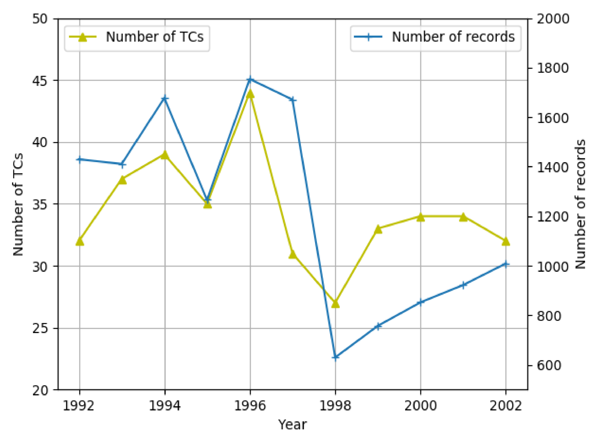
However, because the performances of Methods A and B were unknown for certain years, it would be unfair to compare them with the AE-GRU model when applying data from 1945 to 2017. Therefore, we compared the results per year of our proposed model with those of the NWP model (C), which performed the best among Methods A, B, and C. The NWP model results were from [43]. The comparison results per year are shown in Figure 6. In addition, the number of tropical cyclones and the number of records per year for this comparison are indicated in Figure 7. From Figure 6, it is clear that our proposed model achieved better results than the NWP model for almost every year. For the year 1998, the error of the proposed model peaked, but was still lower than that of the NWP model. According to Figure 7, there were fewer tropical cyclones and records in 1998 than during the other years. The reason for the larger error in 1998 was due to insufficient data, which proved that the AE-GRU model was data-driven. However, the AE-GRU model showed a higher robustness and stability than the NWP method.

4.4.2. Comparison Experiment with Deep Learning Methods

Comparing with traditional deep learning methods, the performances metrics of RNN, AE-RNN, GRU, LSTM and AE-GRU models are shown in

Table 5. Comparison results among RNN, AE-RNN, GRU, and AE-GRU

Method	Predicted Time Range	Test Avg APE	Test Max APE	Test Min APE
RNN [16]	12 h	164.22 km	344.24 km	1.42 km
	24 h	197.52 km	348.67 km	1.47 km
	48 h	177.37 km	348.67 km	2.74 km
	72 h	174.97 km	348.29 km	0.38 km
AE-RNN [44]	12 h	150.36 km	345.39 km	0.78 km
	24 h	164.04 km	347.57 km	2.81 km
	48 h	173.28 km	346.19 km	2.44 km
	72 h	174.67 km	347.46 km	2.03 km
GRU [10]	12 h	171.07 km	347.47 km	3.25 km
	24 h	172.84 km	347.56 km	0.31 km
	48 h	182.04 km	346.13 km	1.04 km
	72 h	175.82 km	348.26 km	2.24 km
LSTM [24]	12 h	173.79km	348.19km	4.71km
	24 h	173.67km	347.95km	0.90km
	48 h	175.02km	342.53 km	2.36 km
	72 h	175.75 km	348.70 km	1.17 km
AE-GRU	12 h	138.67 km	348.27 km	2.55 km
	24 h	143.23 km	347.55 km	0.98 km
	48 h	174.57 km	343.66 km	1.75 km
	72 h	174.62 km	344.96 km	1.91 km

, which includes the average absolute position error, maximum absolute position error, and minimum absolute position error using the test set to forecast a tropical cyclone position at the next 12, 24, 48, and 72 h. The results were predicted using the previous 72 h locations of the tropical cyclones and the meteorological variables, which meant the time step was 12. For each predicted time range, the bold font is used to emphasize the best prediction results. From Table 5, it is evident that the AE-GRU model performed best, the average APE of which in the 12, 24, and 72 h forecasts were the lowest. That is, the predicted locations were closest to the real locations. Moreover, the 12, 24, 48, and 72 h forecasts demonstrated a decreasing performance because the prediction errors were cumulative over time. The max APE of the AE-GRU model was lower than that of the other models for the 24, 48, and 72 h forecasts, with the exception of the RNN, which performed better in the 12 h forecast. This result occurred because the learned information in the RNN-based model could not remember previous information of a long time ago with the increase of time intervals, which made it perform worse in terms of a long prediction time. However, the LSTM- and GRU-based models had memory cells that improved the long-term dependency problem. The best performance of min APE for the 24 and 48 h forecasts was achieved by GRU; however, the largest value of min APE for all five methods was no more than 5 km. In addition, comparing GRU with LSTM, the values of max APE and min APE of the GRU model were lower than the LSTM model. The average APE of GRU performed slightly better than LSTM in the 12 and 24 h forecast. Finally, comparing the AE-RNN and AE-GRU models with the GRU and RNN models alone, the models with an AE layer could achieve a better performance. Therefore, it was necessary to add an AE network to extract deep joint features between the locations and meteorological variables.

On the other hand, to better compare the experimental results of the RNN, AE-RNN, GRU, LSTM, and AE-GRU models, the performance metrics’ values, including MAE, RMSE, and MAPE, are shown in

Table 6. The prediction results of RNN, AE-RNN, GRU, LSTM, and AE-GRU using MAE, RMSE, and MAPE.

Methods	Dataset	Longitude			Latitude
		MAE	RMSE	MAPE	MAE	RMSE	MAPE
RNN [16]	Train	0.006257	0.008113	0.007923	0.006818	0.008588	0.025302
	Validation	0.005498	0.007931	0.007111	0.007245	0.015367	0.029939
	Test	0.00652	0.008556	0.008362	0.00692	0.008948	0.024227
AE-RNN [44]	Train	0.004601	0.006242	0.006486	0.007548	0.010023	0.027295
	Validation	0.004342	0.005721	0.005968	0.00758	0.008988	0.029349
	Test	0.004345	0.005603	0.006106	0.007618	0.009273	0.029999
GRU [10]	Train	0.003822	0.004338	0.003804	0.005096	0.007405	0.019484
	Validation	0.00385	0.003958	0.003767	0.004990	0.010832	0.020406
	Test	0.00388	0.005111	0.003783	0.004931	0.006610	0.017913
LSTM [24]	Train	0.00467	0.00588	0.00664	0.007284	0.00974	0.027391
	Validation	0.00456	0.005394	0.006553	0.0072	0.008636	0.028688
	Test	0.00461	0.00559	0.006517	0.007216	0.008583	0.026491
AE-GRU	Train	0.002585	0.003945	0.003368	0.004158	0.007416	0.0130732
	Validation	0.002757	0.00397	0.003635	0.0041940	0.006921	0.0147232
	Test	0.002627	0.00494	0.003403	0.004313	0.007389	0.012989

. The experiment was implemented to predict tropical cyclone locations at the next 12 h. The best testing results are emphasized in bold font as well. As shown in Table 6, our proposed model performed the best, where almost all performance errors of the testing set were the lowest values. When comparing RNN, LSTM, and GRU models, we could see that both the LSTM and GRU models outperformed the naive RNN model, which indicated that the naive RNN model was inadequate to deal with long-term dependency tropical cyclone tracks. In addition, to compare the GRU model with the LSTM model, we could find that the GRU was more suitable than the LSTM to solve the tropical cyclone track prediction in this study. At last, comparing our proposed model with the GRU-alone model, the performance metrics of our proposed model were slightly better than the GRU-alone model in general. This indicated that all the GRU-based models could achieve good results in predicting tropical cyclones’ tracks. However, our proposed model adding an AE layer to the model could achieve a better generalization capability. Overall, the AE-GRU model was appropriate for predicting tropical cyclones’ tracks, because the auto-encoder layer in this model could extract implicit features from the tropical cyclone tracks and meteorological variables, which could improve the generalization capability and efficiency, and the GRU layer had the ability to deal with time-series prediction and also solved the long time dependency problem in traditional time series models.

To further demonstrate the effectiveness of the model in predicting individual tropical cyclones, the strong typhoons Meranti, Haiyan, Tip, and Dujuan were chosen to visualize the predicted tracks. The results were based on the previous 72 h data to forecast the next 72 h. Figure 8a–d shows the prediction tracks of the typhoons Tip, Meranti, Dujuan, and Haiyan, respectively. The blue lines in these figures indicate the predicted track, and the red lines represent the actual tropical cyclone track. Figure 8 shows that our proposed model could achieve a good performance in predicting strong typhoon tracks when using the tropical cyclone location data and the meteorological variable data. The predicted tracks were close to the real tracks.

Table 7. Avg APE, max APE, and min APE results of four typhoons in the 72 h forecast.

Typhoon	Avg APE	Max APE	Min APE
Tip	188.08 km	323.72 km	67.39 km
Meranti	148.01 km	247.41 km	11.56 km
Dujuan	182.32 km	339.738 km	54.94 km
Haiyan	137.87 km	292.00 km	15.15 km

shows the average APE, max APE, and min APE between the predicted track and the actual track of the target typhoon. The table indicates that the average APEs of all four typhoons were less than 200 km and the maximum APEs were less than 340 km, among which the typhoons Tip and Dujuan had relatively larger errors than the other two typhoons because the typhoon tracks were affected by other factors as well, including the geostrophic deflection force, the location of the subtropical high pressure zone, the influence of cold air, and the topography of the inland areas, which made the learned features from the typhoon tracks and meteorological variables in the AE model insufficient to represent the typhoon features at the current timestamp.

4.4.3. Comparison Experiment on the Effect of Meteorological Variables on the Prediction Results

To validate how each meteorological variable affected the prediction results, several meteorological variables with fewer missing values, combined with the location (longitude and latitude), were used as the model input. There were six different input groups in total, which contained the location only, the location with VMAX, the location with MSLP, the location with MRD, the location with RADP, and the location with all meteorological variables. The experiment was implemented using the proposed AE-GRU model, and the results were predicted using the previous 72 h locations of the tropical cyclones and meteorological variables to forecast 72 h locations. The performance results, including the average APE, max APE, and min APE, are shown in

Table 8. Avg APE, max APE, and min APE of different inputs.

Typhoon	Avg APE	Max APE	Min APE
Location	180.91 km	345.11 km	4.75 km
Location+ VMAX	175.02 km	344.97 km	2.45 km
Location + MSLP	176.29 km	345.83 km	2.10 km
Location + MRD	177.64 km	348.56 km	2.54 km
Location + RADP	176.20 km	347.83 km	1.96 km
Location + all variables	174.62 km	344.96 km	1.91 km

, where the lowest values are emphasized in bold. When no meteorological variables were used as the input data, the average APE and min APE were the highest, which indicated that the forecast result was inferior to the use of meteorological variables. In addition, when all meteorological variables were used, the average APE, min APE, and max APE were the lowest. Moreover, when comparing the variables VMAX, MSLP, MRD, and RADP, the results demonstrated that using VMAX along with the location could achieve the best results, the average APE and min APE of which were the lowest. Overall, all meteorological variables could contribute to tropical cyclone track prediction, and the meteorological variable maximum sustained wind speed (VMAX) was the most effective.

5. Conclusions

In this paper, we addressed the challenge of predicting tropical cyclone tracks under a big data environment. Specifically, a novel fusion deep neural network based on an AE and a GRU was proposed for tropical cyclone track forecasting. The AE layer applied in our proposed model could be used to extract some meteorological factors and trajectory features from the preprocessed data. In addition, it could eliminate data redundancies and increase the model’s generalization capability. A GRU layer was then implemented to extract the nonlinear and complex temporal features from the time-series dataset and then predict tropical cyclone tracks. In general, the AE-GRU model could process the time-sequential data effectively and make an accurate track prediction. Comparative experiments were conducted using the JWTC dataset for the years 1945–2017. The results indicated that our proposed model performed better than a traditional statistic model, a dynamical and numerical model, and a numerical weather prediction model for 24, 48, and 72 h forecasting. In addition, compared with some deep learning models, including an RNN, an AE-RNN, an LSTM, and a GRU, the proposed model also incurred a lower prediction error, the average APE of which was 174.62 km for a 72 h forecast. Furthermore, all meteorological variables showed a positive effect on tropical cyclone track prediction. However, the variable maximum sustained wind speed had the greatest contribution.

In general, the proposed deep learning model was suitable to make tropical cyclone track prediction using historical tropical cyclone landing position data and meteorological variables. However, some limitations remain. First, tropical cyclones with different intensities may affect the landing locations to some extent. Second, the model could only predict tropical cyclone tracks, without the capability of predicting the amount of precipitation, wind speed, and tropical cyclone intensity. Third, the model could predict at most a 72 h tropical cyclone track rather than a longer time range. In the future, we will improve our model by considering tropical cyclone intensities in the deep learning model and adding more datasets to predict more meaningful variables for a longer time period.

References

- The Central People’s Government of the People’s Republic of China. Available online: http://www.gov.cn/xinwen/2018-02/01/content_5262947.htm (accessed on 1 June 2019).
- Yu, J.; Tang, J.; Dai, Y.; Yu, B. Analyses in errors and their causes of Chinese typhoon track operational forecasts. Meteorol. Mon. 2012, 38, 695–700. (In Chinese) [Google Scholar]
- Goerss, J.S. Tropical cyclone track forecasts using an ensemble of dynamical models. Mon. Weather. Rev. 2000, 128, 1187–1193. [Google Scholar] [CrossRef]
- Iwasaki, T.; Nakano, H.; Sugi, M. The performance of a typhoon track prediction model with cumulus parameterization. J. Meteorol. Soc. Jpn. Ser. II 1987, 65, 555–570. [Google Scholar] [CrossRef] [Green Version]
- Xu, Y.L.; Zhang, L.; Gao, S.Z. The advances and discussions on China operational typhoon forecasting. Meteorol. Mon. 2010, 36, 43–49. [Google Scholar]
- Hall, T.M.; Jewson, S. Statistical modelling of North Atlantic tropical cyclone tracks. Tellus A Dyn. Meteorol. Oceanogr. 2007, 59, 486–498. [Google Scholar] [CrossRef] [Green Version]
- He, K.; Zhang, X.; Ren, S.; Sun, J. Deep residual learning for image recognition. In Proceedings of the IEEE Conference on Computer Vision and Pattern Recognition, Las Vegas, NV, USA, 27–30 June 2016; pp. 770–778. [Google Scholar]
- Collobert, R.; Weston, J. A unified architecture for natural language processing: Deep neural networks with multitask learning. In Proceedings of the 25th ACM International Conference on Machine Learning, Helsinki, Finland, 5–9 July 2008; pp. 160–167. [Google Scholar]
- Lange, S.; Riedmiller, M. Deep auto-encoder neural networks in reinforcement learning. In Proceedings of the 2010 IEEE International Joint Conference on Neural Networks (IJCNN), Barcelona, Spain, 18–23 July 2010; pp. 1–8. [Google Scholar]
- Cho, K.; Van Merriënboer, B.; Bahdanau, D.; Bengio, Y. On the properties of neural machine translation: Encoder-decoder approaches. arXiv 2014, arXiv:1409.1259. [Google Scholar]
- Emanuel, K.A. Thermodynamic control of hurricane intensity. Nature 1999, 401, 665. [Google Scholar] [CrossRef]
- Weber, H.C. Hurricane track prediction using a statistical ensemble of numerical models. Mon. Weather. Rev. 2003, 131, 749–770. [Google Scholar] [CrossRef]
- DeMaria, M.; Mainelli, M.; Shay, L.K.; Knaff, J.A.; Kaplan, J. Further improvements to the statistical hurricane intensity prediction scheme (SHIPS). Weather Forecast. 2005, 20, 531–543. [Google Scholar] [CrossRef] [Green Version]
- Davis, C.; Wang, W.; Chen, S.S.; Chen, Y.; Corbosiero, K.; DeMaria, M.; Dudhia, J.; Holl, G.; Klemp, J.; Michalakes, J.; et al. Prediction of landfalling hurricanes with the advanced hurricane WRF model. Mon. Weather Rev. 2008, 136, 1990–2005. [Google Scholar] [CrossRef] [Green Version]
- Grecu, M.; Krajewski, W.F. An efficient methodology for detection of anomalous propagation echoes in radar reflectivity data using neural networks. J. Atmos. Ocean. Technol. 2000, 17, 121–129. [Google Scholar] [CrossRef]
- Alemany, S.; Beltran, J.; Perez, A.; Ganzfried, S. Predicting hurricane trajectories using a recurrent neural network. arXiv 2018, arXiv:1802.02548. [Google Scholar] [CrossRef] [Green Version]
- Moradi Kordmahalleh, M.; Gorji Sefidmazgi, M.; Homaifar, A. A sparse recurrent neural network for trajectory prediction of atlantic hurricanes. In Proceedings of the ACM Genetic and Evolutionary Computation Conference 2016, Denver, CO, USA, 20–24 July 2016; pp. 957–969. [Google Scholar]
- Vohradsky, J. Neural model of the genetic network. J. Biol. Chem. 2001, 276, 36168–36173. [Google Scholar] [CrossRef] [PubMed] [Green Version]
- Chen, J.; Yang, L.; Zhang, Y.; Alber, M.; Chen, D.Z. Combining fully convolutional and recurrent neural networks for 3d biomedical image segmentation. In Proceedings of the Annual Conference on Neural Information Processing Systems 2016, Barcelona, Spain, 5–10 December 2016; pp. 3036–3044. [Google Scholar]
- Lim, S.J.; Jang, S.J.; Lim, J.Y.; Ko, J.H. Classification of snoring sound based on a recurrent neural network. Expert Syst. Appl. 2019, 123, 237–245. [Google Scholar] [CrossRef]
- Chen, L.; Pan, X.; Zhang, Y.H.; Liu, M.; Huang, T.; Cai, Y.D. Classification of Widely and Rarely Expressed Genes with Recurrent Neural Network. Comput. Struct. Biotechnol. J. 2019, 17, 49–60. [Google Scholar] [CrossRef]
- Rather, A.M.; Agarwal, A.; Sastry, V.N. Recurrent neural network and a hybrid model for prediction of stock returns. Expert Syst. Appl. 2015, 42, 3234–3241. [Google Scholar] [CrossRef]
- Xu, K.; Ba, J.; Kiros, R.; Cho, K.; Courville, A.; Salakhudinov, R.; Zemel, R.; Bengio, Y. Show, attend and tell: Neural image caption generation with visual attention. arXiv 2015, arXiv:1502.03044. [Google Scholar]
- Hochreiter, S.; Schmidhuber, J. Long short-term memory. Neural Comput. 1997, 9, 1735–1780. [Google Scholar] [CrossRef]
- Gao, S.; Zhao, P.; Pan, B.; Li, Y.; Zhou, M.; Xu, J.; Zhong, S.; Shi, Z. A nowcasting model for the prediction of typhoon tracks based on a long short term memory neural network. Acta Oceanol. Sin. 2018, 37, 8–12. [Google Scholar] [CrossRef]
- Kim, S.; Kim, H.; Lee, J.; Yoon, S.; Kahou, S.E.; Kashinath, K.; Prabhat, M. Deep-Hurricane-Tracker: Tracking and Forecasting Extreme Climate Events. In Proceedings of the 2019 IEEE Winter Conference on Applications of Computer Vision (WACV), Waikoloa Village, HI, USA, 7–11 January 2019; pp. 1761–1769. [Google Scholar]
- Minh, D.L.; Sadeghi-Niaraki, A.; Huy, H.D.; Min, K.; Moon, H. Deep learning approach for short-term stock trends prediction based on two-stream gated recurrent unit network. IEEE Access 2018, 6, 55392–55404. [Google Scholar] [CrossRef]
- Zhao, R.; Wang, D.; Yan, R.; Mao, K.; Shen, F.; Wang, J. Machine health monitoring using local feature-based gated recurrent unit networks. IEEE Trans. Ind. Electron. 2017, 65, 1539–1548. [Google Scholar] [CrossRef]
- Hidasi, B.; Quadrana, M.; Karatzoglou, A.; Tikk, D. Parallel recurrent neural network architectures for feature-rich session-based recommendations. In Proceedings of the 10th ACM Conference on Recommender Systems, Boston, MA, USA, 15–19 September 2016; pp. 241–248. [Google Scholar]
- Ravanelli, M.; Brakel, P.; Omologo, M.; Bengio, Y. Light gated recurrent units for speech recognition. IEEE Trans. Emerg. Top. Comput. Intell. 2018, 2, 92–102. [Google Scholar] [CrossRef] [Green Version]
- Su, X. Using Deep Learning Model for Meteorological Satellite Cloud Image Prediction. Agu Fall Meet. Abstr. 2017, 2017, IN13B-0064. [Google Scholar]
- Liu, T.; Li, Z.; Yu, C.; Qin, Y. NIRS feature extraction based on deep auto-encoder neural network. Infrared Phys. Technol. 2017, 87, 124–128. [Google Scholar] [CrossRef]
- Shao, H.; Jiang, H.; Zhao, H.; Wang, F. A novel deep autoencoder feature learning method for rotating machinery fault diagnosis. Mech. Syst. Signal Process. 2017, 95, 187–204. [Google Scholar] [CrossRef]
- Meng, Q.; Catchpoole, D.; Skillicom, D.; Kennedy, P.J. Relational autoencoder for feature extraction. In Proceedings of the 2017 IEEE International Joint Conference on Neural Networks (IJCNN), Anchorage, AK, USA, 14–19 May 2017; pp. 364–371. [Google Scholar]
- Almansor, E.H.; Al-Ani, A. A Hybrid Neural Machine Translation Technique for Translating Low Resource Languages. In Proceedings of the International Conference on Machine Learning and Data Mining in Pattern Recognition, New York, NY, USA, 15–19 July 2018; Springer: Cham, Switzerland, 2018; pp. 347–356. [Google Scholar]
- Krishna, G.; Tran, C.; Yu, J.; Tewfik, A.H. Speech Recognition with no speech or with noisy speech. arXiv 2019, arXiv:1903.00739. [Google Scholar]
- Hidasi, B.; Karatzoglou, A.; Baltrunas, L.; Tikk, D. Session-based recommendations with recurrent neural networks. arXiv 2015, arXiv:1511.06939. [Google Scholar]
- Western North Pacific Ocean Best Track Data. Available online: http://www.metoc.navy.mil/jtwc/jtwc.html?western-pacific (accessed on 15 January 2019).
- Acosta, L.A.; Eugenio, E.A.; Macandog, P.B.; Magcale-Macandog, D.B.; Lin, E.K.; Abucay, E.R.; Cura, A.L.; Primavera, M.G. Loss and damage from typhoon-induced floods and landslides in the Philippines: Community perceptions on climate impacts and adaptation options. Int. J. Glob. Warm. 2016, 9, 33–65. [Google Scholar] [CrossRef]
- Roy, C.; Kovordnyi, R. Tropical cyclone track forecasting techniques DA review. Atmos. Res. 2012, 104, 40–69. [Google Scholar] [CrossRef] [Green Version]
- Jeffries, R.A.; Miller, R.J. Tropical Cyclone Forecasters Reference Guide 3. Tropical Cyclone Formation; Tech. Rep. No. NRL/PU/7515-93-0007; NRL: Monterey, CA, USA, 1993. [Google Scholar]
- Demaria, M.; Aberson, S.D.; Ooyama, K.V.; Lord, S.J. A nested spectral model for hurricane track forecasting. Mon. Weather Rev. 1992, 120, 1628–1643. [Google Scholar] [CrossRef] [Green Version]
- Goerss, J.S.; Sampson, C.R.; Gross, J.M. A history of western North Pacific tropical cyclone track forecast skill. Weather Forecast. 2004, 19, 633–638. [Google Scholar] [CrossRef]
- Srivastava, N.; Mansimov, E.; Salakhudinov, R. Unsupervised learning of video representations using lstms. In Proceedings of the 32th ICML, Lille, France, 6–11 July 2015; pp. 843–852. [Google Scholar]
Figure 1.
Structure of the AE-GRU model.