Histogram-Based Descriptor Subset Selection for Visual Recognition of Industrial Parts

Abstract

This article deals with the 2D image-based recognition of industrial parts. Methods based on histograms are well known and widely used, but it is hard to find the best combination of histograms, most distinctive for instance, for each situation and without a high user expertise. We proposed a descriptor subset selection technique that automatically selects the most appropriate descriptor combination, and that outperforms approach involving single descriptors. We have considered both backward and forward mechanisms. Furthermore, to recognize the industrial parts a supervised classification is used with the global descriptors as predictors. Several class approaches are compared. Given our application, the best results are obtained with the Support Vector Machine with a combination of descriptors increasing the F1 by $0.031$ with respect to the best descriptor alone.

1. Introduction

Computer vision, in the last years, has gained much interest in many fields, such as autonomous driving [1], medical [2], face recognition [3], object detection [4], and object segmentation [5]. Perception is also regarded as one of the key enabling technologies for extending the robot capabilities, preferentially targeting flexibility, adaptation, and robustness, as required for fulfilling the industry 4.0 paradigm [6]. Although in most fields large and complex datasets can be obtained, detection of industrial parts has a lack of datasets. One of the reasons is that most of the time in industrial context, the aim is to detect an object from which usually the CAD is available. However, sometimes there is a need of detecting diverse, complex, and tiny objects [7] and lack of time to generate a robust dataset (taking pictures and labeling). One of the solutions is to generate simulated data to train the models but usually there is a significant gap transferring that learned knowledge to reality.

To make matter worse, industrial parts are usually texture-less. This means that many of the most used recognition methods cannot deal with them. One of the methods to deal with texture-less objects are Convolutional Neural Networks. Nowadays, computer vision researches are mainly focused on using Convolutional Neural Networks (CNN) [8,9,10]. One of the disadvantages of the CNNs is the need of a large dataset to train them. Even if it is possible to use the CNN trained on other fields in industry [11], there is still a need of a large enough training dataset to obtain good results. Feature descriptors based on classical methods have been very useful and thoroughly spread in the literature previous to CNN. One of the benefits of using this approach is that there is no need of a large training set to obtain good results. Actually, there are many image descriptors and each of them has its advantages and disadvantages.

Our approach is based in the idea that the combination of different descriptors leads to a better performance, taking advantage of the benefits of each descriptor to deal with the two problems mentioned before (lack of a large dataset and texture-less objects). The crux of the matter is to select the descriptors that contribute to achieve a better result and discard those that do not provide any improvement. Our method achieves a classification quality similar to state-of-the-art methods on the experiments done.

In Section 2, we present a background of the description methods, classifiers, and features subset selection techniques. In Section 3, we explain the combination of the descriptors and the image classification. The experiments done and their results are gathered in Section 4. Finally, in Section 5, the conclusions are summarized.

2. Background

The analysis of images usually relies on the extraction of visual features. Such an approach can be observed in classification [12], object detection [4], and segmentation [5]. In this section, we provide an overview of the main feature descriptors, together with some of the related classification techniques.

2.1. Features Descriptors

Local features extractors are characteristic local primitives as points focusing on a close neighborhood. Some examples of those features are SIFT [13], SURF [14], and LBP [15]. Global descriptors, instead, extract information directly from the whole image by computing histograms for example. Local features are good for image recognition as each point is independent from the rest and the features are more discriminant. Global features instead are more used for classification and object detection as they achieve a more global representation. Nevertheless, small changes have a larger impact on global features and a better preprocessing is needed when using them. Extracting global features and their classification is usually faster.

As a matter of a fact, combining both local and global features usually performs better [16]. Many researchers use histograms of local features to obtain benefits of both types. Doing so, we obtain a global representation of the local features. [16] present a taxonomy called Histogram of Equivalent Patterns (HEP) that gathers those histograms of local features. In order for a feature to be part of this framework, it needs to have a delimited quantification, that is, the number of possible values of the extracted feature must be small enough to obtain a relevant histogram. For example, LBP [15] is part of this framework as the possible values are 256 so the resulting histogram is of length 256, while HOG or SIFT are not part of the HEP framework as the number of possible values is high and the resulting histogram is not relevant. In [17], a combination of descriptors was also used, but limited to local descriptors.

One of the first HEP methods was introduced in 1973. This method, called Gray Level Co-occurrences Matrices (GLCM) [18] measures the joint probability of the gray levels of two pixels standing in some predefined relative positions. Since 1973, it has been widely used in many texture analysis applications as a feature extractor in this context.

In 1990, [19] proposed the texture spectrum (TS), which inspired many HEP methods. This texture descriptor is based in decomposing the image into a set of essential small units, called Texture Units (TUs). The occurrence distribution of TU is the TS. One of the first and most used TU-based descriptors is the Local Binary Pattern (LBP) [15]. This last one is a two-level TU, gray-scale invariant and easily combined with a simple contrast measure. One of the main characteristics is its robust invariant to light changes.

Another method based in the TU is the Simplified Texture Unit (STU) [20]. This method use a more reduced range of values without a significant loss of the characterization power. This way, there are two options of STU: using the crosswide neighbors (up, right, down, and left) and using diagonal neighbors (up-left, up-right, down-right, and down-left); its reduced length is commonly used in real-time applications obtaining similar performance to LBP.

The modified texture spectrum (MTS) [21] can be considered as a simplified version of LBP, where only a subset of the peripheral pixels (up-left, up, up-right, and right) are considered. Its TS is 16 elements in length, significantly improving the computation efficiency on classification. Similarly to STU, the reduction on the TS length leads to a faster classification while achieving similar performance.

The GaborLBP [22] considers the advantages of the Gabor filters in computer vision and exploits them. It first applies a Gabor transformation and encodes the magnitude values with the LBP operator. Fusing both tools enables handling of illumination changes, viewpoint angle changes, and non-rigid bodies. Usually this combination is used for face recognition or person identification.

The Local Ternary Pattern (LTP) [23] is a generalization of the LBP and it is more discriminant and less sensitive to noise in uniform regions. It is a local texture descriptor that uses a 3-value coding that thresholds around zero. Comparing to the LBP, LTP is more resistant to noise but no longer invariant to gray-level transformations.

The Binary Gradient Contours (BGC) [24] is a binary 8-tuple. It relies on computing a set of eight binary gradients between pairs of pixels all along a closed path around the central pixel of a 3 × 3 grayscale image patch. They defined the closed path in three different ways: single-loop (BGC1), double-loop (BGC2), and triple-loop (BGC3).

Another HEP descriptor, is the Local Quantized Patterns (LQP) [25]. This is a generalization of local pattern features that makes use of vector quantization. It uses large local neighbourhoods and/or deeper quantization with domain-adaptative vector quantization.

The Weber’s Law Descriptor (WLD) [26] was proposed in 2010 as a simple, yet very powerful and robust descriptor. It is based on the fact that human pattern perception also depends on the original intensity of the stimulus and not only on the change of a stimulus (such as sound and lighting). It is composed of two components: differential excitation and orientation.

The Histogram of oriented gradients (HOG) [27] is a feature descriptor that counts the occurrences of gradient orientation in localized portions of an image. Operating on local cells provides invariation to geometric and photometric transformations. The HOG descriptor is particularly suited for human detection in images. Even if HOG is not part of HEP, the way it generates the descriptor (calculating a histogram of gradients) works similar to HEP methods so it can be used similarly.

2.2. Classifiers

Descriptors are used to obtain features from images. Those features are then used by the classifiers to predict which object is on each image. Many machine learning algorithms are used for classifying images, but some of the most popular ones are K-Nearest Neighbors, Naive Bayes, Random Forest, Support Vector machine, Random Committee, Bagging, and Multiclass Classifier.

The Nearest Neighbor Rule is a well-known algorithm and the simplest nonparametric decision procedure that assigns to the uncategorized object the label of the closest sample of the training set. In 1967, a modification of this algorithm led to one of the most used classification algorithms, the K-Nearest Neighbors (KNN) [28]. It is based on looking for closest points and classifying them as the majority class. For a given set of n pairs $(x_1,{\theta }_1),\dots ,(x_n,{\theta }_n)$, where $x_i$ is in a metric space X and ${\theta }_i$ is the category that $x_i$ belongs to from a subset $\{1,2,\dots ,M\}$, a new arriving instance x is analyzed to estimate its corresponding class $\theta$. This estimation is done by looking for the nearest neighbor $X_n^{\prime }\in (x_1,x_2,\dots ,x_n)$:

$$mind(x_i,x)=d(x_n^{\prime },x)i=1,2,\dots ,n$$

where d is a distance metric according to the space X. The new instance x will be assigned to the category ${\theta }_n^{\prime }$. This is the basic 1-NN. In general, KNN rule decides x belongs to the category of majority vote of the nearest k neighbors.

The Naive Bayes [29], the simplest Bayesian classifier, is another classification algorithm that is often used for its simplicity. It is based on the Bayesian Rule and assumes that variables are independent given the class. Despite this unrealistic assumption, it is successful in practice. The Bayesian rule states that the probability that a instance x belongs to class $C_k$ is

$$P\left(C_k\right|\mathbf{x})=\frac{P\left(C_k\right)P\left(\mathbf{x}\right|C_k)}{P\left(\mathbf{x}\right)}$$

(1)

where $C_k$ is the class between the K possible classes and x the instance to be classified. Taking into account the independence assumption, the conditional distribution over the class variable C is

$$p\left(C_k\right|x_1,\dots ,x_n)=\frac{1}{Z}p\left(C_k\right)\prod _{i=1}^{n}p\left(x_i\right|C_k)$$

(2)

The instance is classified as the class with more $p\left(C_k\right|x_1,\dots ,x_n)$.

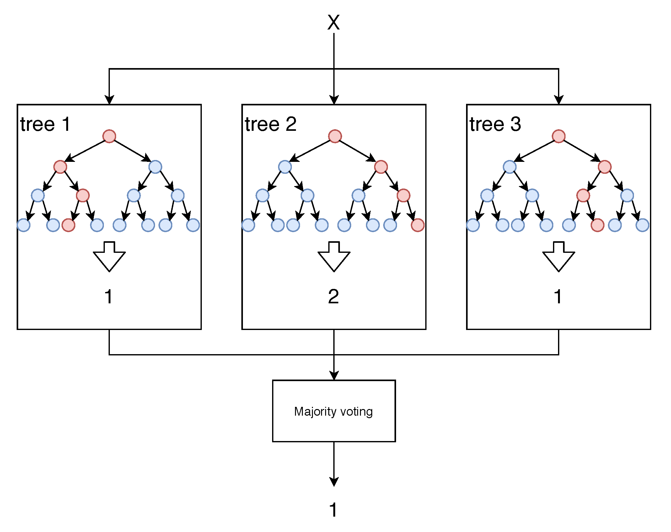
The Random Forest (RF) [30] is a combination of decision trees that use random subsets of the features to be built. Figure 1 shows an example of RF.

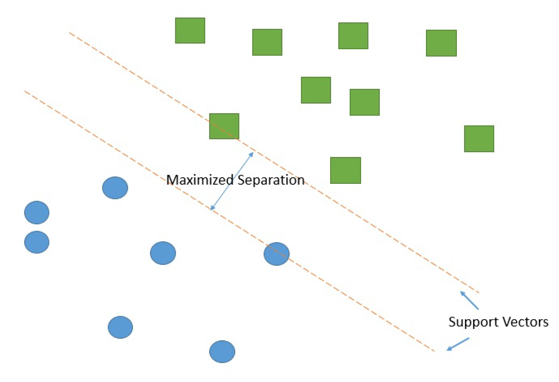
Support Vector Machines (SVM) [31] are supervised learning models that look for optimal hyperplanes that separates classes. An optimal hyperplane is defined as the linear decision function with maximal margin between the vectors of the two classes (Figure 2).

Random Committee (RC) [32] is a committee of random classifiers. The base randomizable classifiers (that form the committee members) are built using different random number seeds based in the same data. The final prediction is a straight average of the predictions generated by the individual base classifiers.

The Bagging [33] technique is called after Bootstrap aggregating. This machine learning ensemble that can be used to improve the stability of a model by improving the accuracy and reducing variance in order to reduce overfitting.

2.3. Feature Selection

As stated before, the crux of the matter in this paper relies on how to select the different visual features to improve the individual score of each descriptor. Some authors have used different techniques to do this [34,35]. Feature Selection is a machine learning technique that is used in many fields and usually improves the accuracy of the model. In [34], the authors uses different feature selection techniques to improve the score in the Quantitative Structure–Activity Relationship (QSAR). In [35], instead, they use a similar approach for hand pose recognition. In [36], a view over the different feature selection techniques and its variations is described. Our approach is based in those methods and is used in a completely different context.

3. Proposed Approach

In order to achieve a better performance than just using a single global descriptor, we propose using a Descriptor Subset Selector. That is, we try to find the combination of global descriptors that scores a better result. Among all available options of subset selection, we have used 2 for their greedy approach which achieve a significant performance: forward selection and backward selection. First, we present the classification of a single image, given a descriptor and a classifier. After that, we explain the feature selection techniques to choose the combination of descriptor to use. Next, we present the evaluation methods, in order to decide which is the best solution. Finally, we present the whole pipeline of the proposed approach.

3.1. Classification

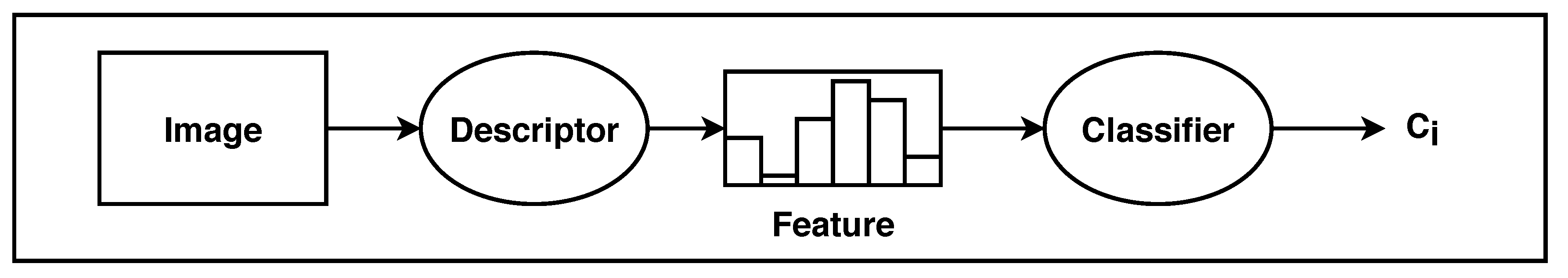
The first step in the pipeline is to classify a picture into the C different classes. Given a descriptor and a classifier, the classifier is trained with features obtained from the description of the set of images for training. Given a new image to be classified, the descriptor extracts the feature from the image and that feature is classified by the classifier (Figure 3).

3.2. Feature Selection Techniques

The feature selection techniques are used to chose the descriptors for the classification. An exhaustive search of best combination of descriptors is computationally inefficient, while it guarantees that the optimal solution is achieved. Nevertheless, a suboptimal solution can be achieved using a sequential search. This is an iterative search that once a stage of the search is reached, is impossible to go back. The complexity of the exhaustive search is exponential ($O\left(2^n\right)$), while the sequential search remains polynomial ($O\left(n^{k+1}\right)$), where k is the number of evaluated subsets in each stage. This last one does not guarantee an optimal solution.

Another important consideration in the feature selection techniques is the generation of the successors, i.e., how to select the next candidates for the following stage. The simplest and most used methods are Forward and Backward generation [36]. In forward generation, on each stage the element which makes J (the evaluation measure) greater is selected and added to the selected subset. For example, the first descriptor added to the subset would be the one with the best individual score. The next stage would add to the subset the one that concatenated with the previous one makes the score greater. We refer to this method as Sequential Forward Subset Selection (SFSS) [36], and its pseudocode is described in Algorithm 1. The backwards is the opposite behavior. The subset is initialized with all the elements and on each stage the element that that makes J greater when removed is done so. The stopping criteria in both cases can be that J is not increased in j steps or the subset achieves a desired length. We refer to this method as Sequential Backward Subset Selection (SBSS) [36], and its pseudocode is described in Algorithm 2.

Algorithm 1: Sequential Forward Subset Selection

where ∪ stands for union between two sets or an element and a set and ∖ operator stands for difference.

Algorithm 2: Sequential Backward Subset Selection

3.3. Evaluation Measure

A classification quality can be quantified using measures such the one of Equation (3). This measure, named F-value [37] or F-score, is an evaluation measure that takes into account the precision and the recall. More precisely, the metric used is a particular case of the F-value where the precision and the recall are balanced. This is called $F_1$, an harmonic mean between the precision and the recall.

$$F_1\left(y\right)=2·\frac{precisio{n}_y\ast recal{l}_y}{precisio{n}_y+recal{l}_y}$$

(3)

where y refers to a class (also referred in this paper as $C_i$). $F_1$ is class-dependent, so for each class, y, the precision and the recall are computed for that class. The precision (Equation (4)) is the ratio between the correctly predicted views with label y ($t{p}_y$ or true positive) and all predicted views for that given instance ($\left|\psi \right(X)=y|$). The recall (Equation (5)), instead, is the relation between correctly predicted views with label y ($t{p}_y$ or true positive) and all views that should have that label ($\left|label\right(X)=y|$).

$$precisio{n}_y=\frac{t{p}_y}{\left|\psi \right(X)=y|}$$

(4)

$$recal{l}_y=\frac{t{p}_y}{\left|label\right(X)=y|}$$

(5)

To evaluate each stage of the feature selection we use the averaged $F_1$. This is the mean of the $F_1$’s of all the classes (Equation (6)).

$$F_1=\frac{1}{\left|Y\right|}\sum _{y\in Y}{F}_1\left(y\right)$$

(6)

3.4. Full Pipeline

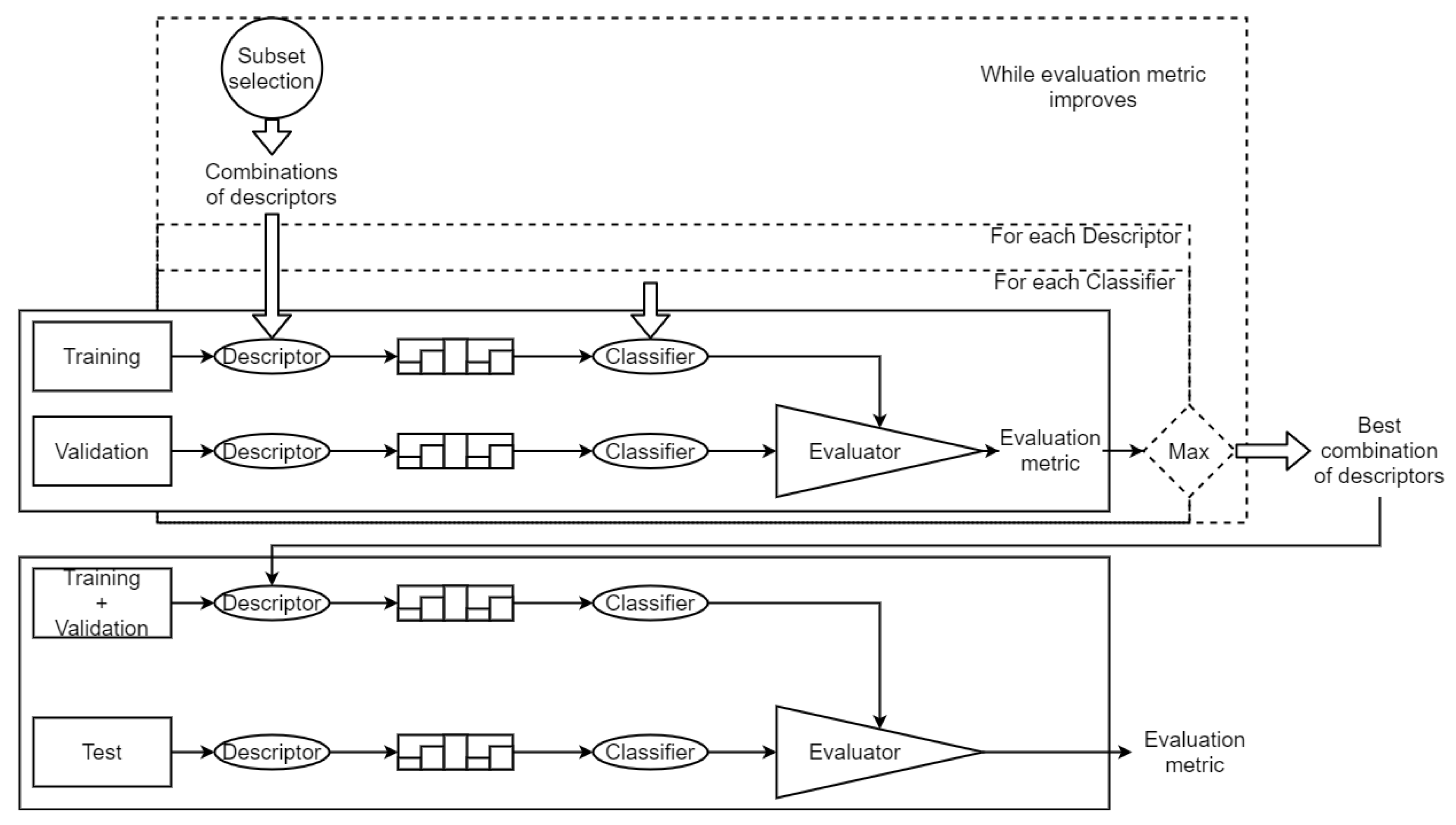
The dataset is divided in two sets: training and test. During the search of the best combination of descriptors, training set is used for training the classifiers and validate the feature selection technique. This separation is made by a Leave-One-Out Cross-Validation (LOOCV) [38]. Each image of the set is used as validation while the rest of the set is used to train the model. Figure 4 shows the whole process. Given a descriptor and a classifier, both are tested using the LOOCV to set the training and validation sets. Once the best combination of descriptors is found, to test the quality of this combination, we use the test set to obtain a general evaluation metric.

4. Experiments and Results

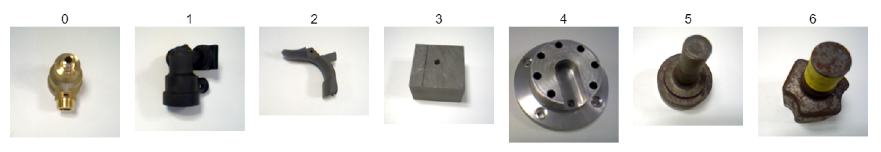
As stated before, the aim of this paper is to present a method to improve the accuracy on reduced datasets of texture-less objects. In order to prove that our method improves the score of the descriptors by their own, we have created a small dataset composed by seven different random industrial parts (Figure 5). We took 50 pictures of each industrial part taken from different viewpoints and different illumination conditions. Objects are rotated and translated but all images are free from occlusion, and with an empty and white background.

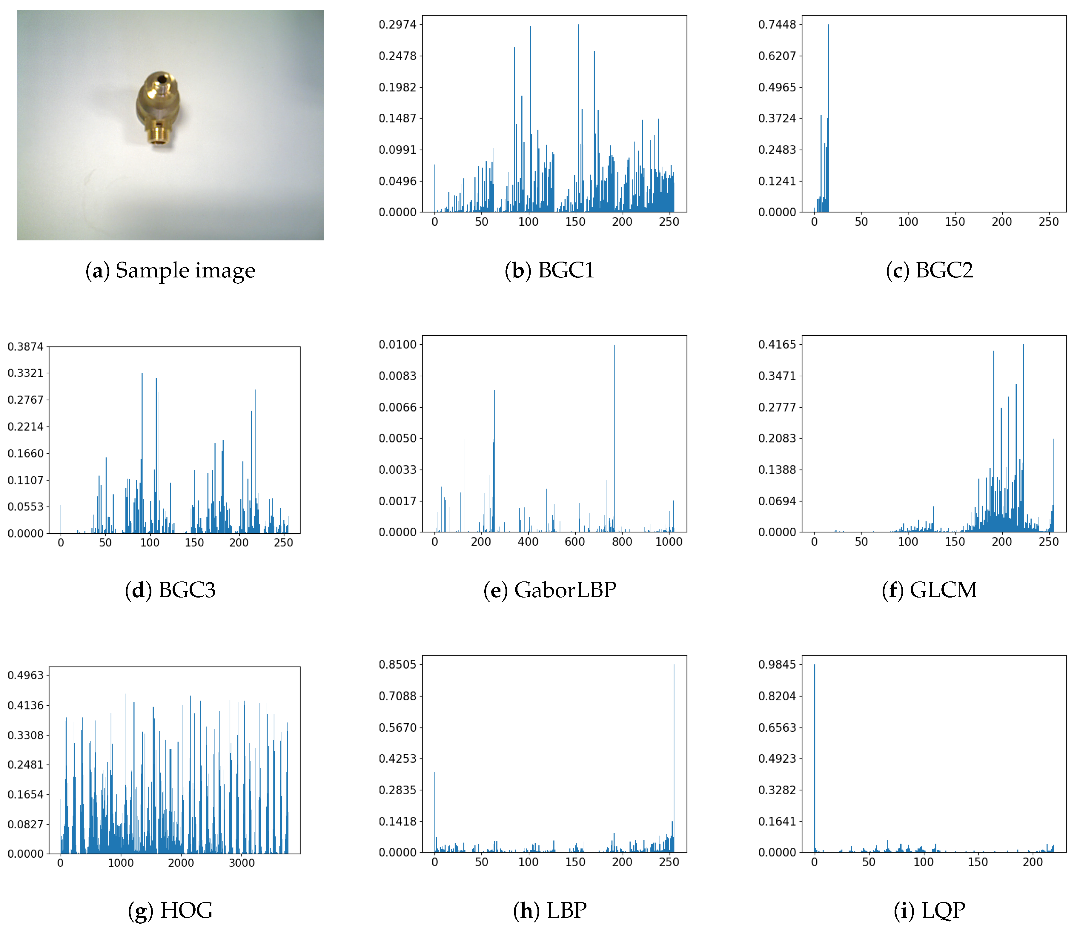
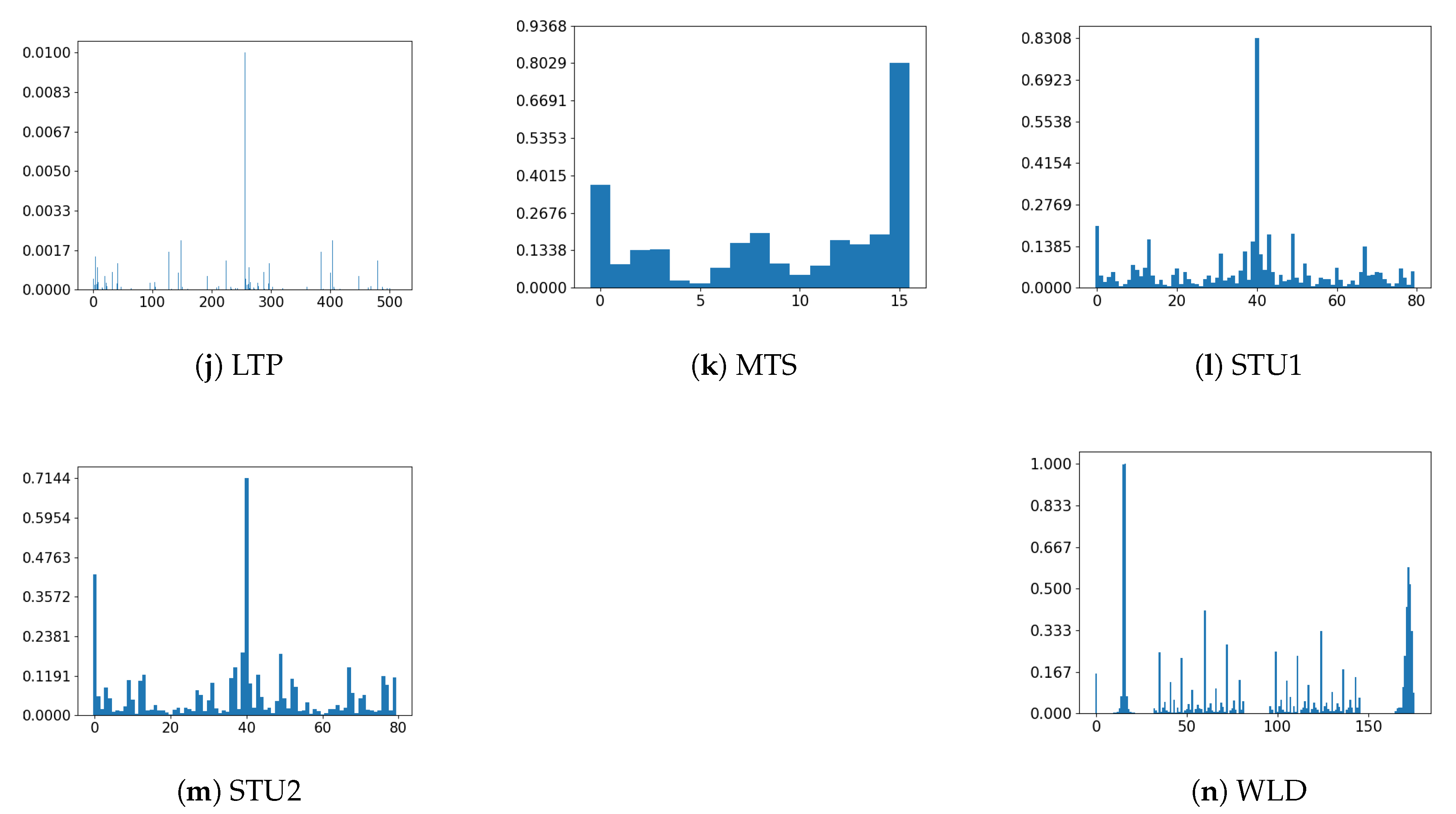
Our pool of descriptors D for discovering the best combination is made up of BGC1 BGC2, BGC3, LBP, GaborLBP, GLCM, HOG, LQP, LTP, MTS, STU+ (or STU1), STU × (or STU2), and WLD. All descriptors but HOG are computed on grids of different sizes: $1\times 1$, $4\times 4$, and $8\times 8$. The length of gridded histograms is the length of the descriptor multiplied by the number of grids. The HOG is applied to the whole image directly. Figure 6 shows a sample image from our database that has been described by each of the descriptors.

The classifiers used are KNN, NB, SVM 1-vs-1 trained with SMO (Sequential Minimal Optimization [39]), SVM 1-againt-all trained with SGD (Stochastic Gradient Descent [40]), RC, RF, and Bagging. To distinguish between the two SVM implementations, we call SVM to the one trained with SMO and SVM-SGD to the other one. In terms of performance, some of the classifiers are drastically affected by the parameters, but tuning the parameters makes a complex casuistry which is not the aim of this paper. Used parameters are standards and those are given in the Appendix A. The results are obtained for a Intel Xeon CPU of 3GHz and 16GB of RAM, and no GPU acceleration has been used. The following subsections explain the results obtained in the experiments.

4.1. Forward Subset Selection

Forwards Subset Selection of descriptors applied to the whole image (from now on, FSS$1\times 1$) experiments results are shown in

Table 1. Forward Subset Selection of descriptors applied to the whole image (also known as FSS$4\times 4$). Level 1 uses only one descriptor. The following levels concatenate the best descriptor from the previous level to the rest of the descriptors. The algorithm stops on level 4 because the evaluation measure is not improved from level 3 to 4.

Descriptor	Level 1	Level 2	Level 3	Level 4
		WLD +	WLD + BGC2 +	WLD + BGC2 + MTS +
BGC1	0.66 (RF)	0.931 (RF)	0.937 (SVM)	0.934 (SVM/RF)
BGC2	0.489 (SVM)	0.969 (SVM)	—	—
BGC3	0.611 (SVM)	0.937 (RC)	0.929 (RF)	0.929 (RF)
GaborLBP	0.671 (RF)	0.931 (RF)	0.903 (RF)	0.906 (RF)
GLCM	0.811 (RF)	0.951 (RF)	0.903 (RF)	0.963 (SVM)
HOG	0.84 (SVM)	0.923 (SVM)	0.923 (SVM)	0.923 (SVM)
LBP	0.611 (RF)	0.946 (RF)	0.917 (SVM)	0.923 (RF)
LQP	0.697 (RF)	0.949 (SVM)	0.954 (SVM)	0.949 (SVM)
LTP	0.563 (RF)	0.966 (SVM)	0.969 (SVM)	0.966 (SVM)
MTS	0.666 (KNN)	0.966 (SVM)	0.971 (SVM)	—
STU1	0.746 (SVM)	0.951 (SVM)	0.951 (SVM)	0.948 (SVM)
STU2	0.74 (SVM)	0.951 (SVM)	0.957 (SVM)	0.957 (SVM)
WLD	0.94 (RF)	—	—	—

. In Table 1, the classifier that is between brackets is the one that achieves the highest mean score. If we would use the best descriptor alone, the $F_1$ would be $0.94$ with WLD. By combining it with BGC2 and MTS, and using SVM as classifier, we are able to augment quality of $3\%$ to reach $0.971$. On first iteration WLD outperforms the other descriptors with a difference of $0.1$ comparing to the next best descriptor. The second iteration increases the overall accuracy and in almost all the cases improves the accuracy of the previous iteration best case.

Table 2. Forward Subset Selection of descriptors applied to $4\times 4$ gridded image (also known as $FSS4\times 4$).

Descriptor	Level 1	Level 2	Level 3
		STU1 +	STU1 + WLD +
BGC1	0.877 (SVM)	0.908 (SVM-SGD)	0.934 (SVM)
BGC2	0.903 (SVM)	0.931 (SVM)	0.969 (SVM)
BGC3	0.857 (SVM)	0.906 (SVM)	0.931 (SVM)
GaborLBP	0.834 (SVM)	0.883 (SVM)	0.903 (SVM)
GLCM	0.923 (RF)	0.957 (SVM)	0.966 (SVM)
HOG	0.846 (KNN)	0.917 (SVM)	0.94 (SVM)
LBP	0.874 (SVM)	0.906 (SVM)	0.929 (SVM)
LQP	0.911 (SVM)	0.94 (SVM)	0.969 (SVM)
LTP	0.889 (SVM)	0.931 (SVM)	0.96 (SVM)
MTS	0.909 (SVM)	0.94 (SVM)	0.96 (SVM)
STU1	0.934 (SVM)	—	—
STU2	0.914 (SVM)	0.931 (SVM)	0.96 (SVM)
WLD	0.931 (SVM)	0.969 (SVM)	—

shows the results of the Forwards Subset Selection of descriptors applied to a $4\times 4$ grid (FSS$4\times 4$). On average, the first iteration performs better than the non-gridded version FSS$4\times 4$, but the last iteration does not improve the results obtained with FSS$4\times 4$. The first iteration achieves an $F_1$ of $0.934$ and the final iteration $0.969$. Therefore, an improvement of $3.5\%$ is obtained. The final combination of descriptors, the one which achieves the highest score, is composed by STU1 and WLD.

Table 3. Forward Subset Selection of descriptors applied to $8\times 8$ gridded image (also known as $FSS8\times 8$).

Descriptor	Level 1	Level 2	Level 3
		WLD +	WLD + MTS +
BGC1	0.845 (SVM)	0.877 (SVM)	0.897 (SVM)
BGC2	0.911 (SVM)	0.954 (SVM)	0.957 (SVM)
BGC3	0.843 (SVM)	0.863 (RC)	0.877 (SVM)
GaborLBP	0.783 (SVM)	0.849 (Bagging)	0.869 (Bagging)
GLCM	0.909 (SVM)	0.92 (SVM)	0.923 (SVM)
HOG	0.846 (KNN)	0.923 (SVM)	0.909 (SVM)
LBP	0.831 (SVM)	0.886 (Bagging)	0.889 (Bagging)
LQP	0.897 (SVM)	0.929 (SVM)	0.931 (SVM)
LTP	0.9 (SVM)	0.951 (SVM)	0.954 (SVM)
MTS	0.903 (SVM)	0.96 (SVM)	—
STU1	0.921 (SVM)	0.94 (SVM)	0.949 (SVM)
STU2	0.917 (SVM)	0.929 (SVM)	0.937 (SVM)
WLD	0.94 (RF)	—	—

shows the results for the $8\times 8$ gridded version (FSS$8\times 8$). The results are similar to the ones obtained in FSS$4\times 4$. The first iteration achieves an $F_1$ of $0.94$, while the last one achieves a score of $0.96$. In this case, the improvement is $2\%$.

The performance of the 3 options of the parameters are similar but the speed of the classification is much faster with the FSS$1\times 1$ version because the length of the final descriptor is shorter. Therefore, the value of the grid parameter makes not a significant difference in the performance. The recommendation is to use the FSS$1\times 1$.

Regarding the classifiers, in almost all the cases the best classifier is the SVM, which is more evident as the number of descriptors concatenated raises. This is because SVM works well with high dimensionality. Our recommendation is to use SVM trained with SMO.

4.2. Backward Subset Selection

The Backward Subset Selection has a similar behavior.

Table 4. Backward Subset Selection of descriptors applied to $1\times 1$ gridded image (also known as BSS$1\times 1$). Level 1 uses all the descriptors in set D concatenated. Level 2 uses the concatenation of the descriptors in D without each of the descriptors. The following levels use the concatenation of the descriptors in D without the descriptor that makes score higher of the previous level.

Descriptor	Level 1	Level 2	Level 3	Level 4	Level 5	Level 6
	D	D\	D\ GaborLBP +	D\ GaborLBP + HOG +	D\ GaborLBP + HOG + BGC1 +	D\ GaborLBP + HOG + BGC1 + LBP +
BGC1	0.917 (SVM)	0.92 (SVM)	0.923 (SVM)	0.929 (SVM)	—	—
BGC2		0.914 (SVM)	0.92 (SVM)	0.92 (RF)	0.937 (SVM)	0.931 (SVM)
BGC3		0.917 (SVM)	0.92 (SVM)	0.929 (SVM)	0.934 (SVM)	0.937 (SVM)
LBP		0.914 (SVM)	0.92 (SVM)	0.926 (RF)	0.937 (SVM)	—
GaborLBP		0.92 (SVM)	—	—	—	—
GLCM		0.914 (SVM)	0.914 (SVM)	0.92 (SVM)	0.929 (SVM)	0.923 (SVM)
HOG		0.903 (SVM)	0.923 (SVM)	—	—	—
LQP		0.917 (RF)	0.92 (SVM)	0.923 (SVM)	0.923 (SVM)	0.934 (SVM)
LTP		0.909 (SVM)	0.92 (SVM)	0.92 (RF)	0.926 (SVM)	0.929 (SVM)
MTS		0.914 (SVM)	0.92 (SVM)	0.923 (SVM)	0.929 (SVM)	0.931 (SVM)
STU1		0.917 (SVM)	0.92 (SVM)	0.923 (RF)	0.923 (SVM)	0.926 (SVM)
STU2		0.914 (SVM)	0.92 (SVM)	0.926 (RF)	0.931 (SVM)	0.926 (SVM)
WLD		0.914 (SVM)	0.891 (SVM)	0.82 (RF)	0.834 (RF)	0.934 (RF)

shows the results of the Backward Subset Selection of descriptors applied to the whole image (BSS$1\times 1$). This is the case with more iterations. It increases the accuracy from $0.917$ to $0.937$. The resulting descriptor set is composed by BGC2, BGC3, GLCM, LQP, LTP, MTS, STU1, STU2, and WLD.

Table 5. Backward Subset Selection of descriptors applied to $4\times 4$ gridded image (also known as BSS$4\times 4$).

Descriptor	Level 1	Level 2	Level 3	Level 4
	D	D \	D \ LBP +	D \ LBP + STU1 +
BGC1	0.943 (SVM)	0.95 (SVM)	0.951 (SVM)	0.949 (SVM)
BGC2		0.946 (SVM)	0.951 (SVM)	0.954 (SVM)
BGC3		0.949 (SVM)	0.95 (SVM)	0.945 (SVM)
LBP		0.951 (SVM)	—	—
GaborLBP		0.946 (SVM)	0.951 (RF)	0.949 (RF)
GLCM		0.937 (SVM)	0.937 (SVM)	0.94 (SVM)
HOG		0.94 (SVM)	0.943 (SVM)	0.946 (SVM)
LQP		0.946 (RF)	0.946 (SVM)	0.946 (SVM)
LTP		0.946 (SVM)	0.951 (SVM)	0.949 (SVM)
MTS		0.946 (SVM)	0.951 (SVM)	0.954 (SVM)
STU1		0.946 (SVM)	0.954 (SVM)	—
STU2		0.949 (SVM)	0.95 (SVM)	0.949 (SVM)
WLD		0.946 (SVM)	0.946 (SVM)	0.946 (SVM)

shows the results of the Backward Subset Selection of descriptors applied to $4\times 4$ gridded images (BSS$4\times 4$). This time, the improvement is from $0.943$ to $0.954$. The resulting descriptor set is BGC1 BGC2, BGC3, GaborLBP, GLCM, HOG, LQP, LTP, MTS, STU2, and WLD.

Table 6. Backward Subset Selection of descriptors applied to $8\times 8$ gridded image (also known as BSS$8\times 8$).

Descriptor	Level 1	Level 2	Level 3	Level 4	Level 5
	D	D\	D\ LBP +	D\ LBP + GaborLBP +	D\ LBP + GaborLBP + BGC3 +
BGC1	0.92 (SVM)	0.914 (SVM)	0.923 (SVM)	0.943 (SVM)	0.931 (SVM)
BGC2		0.909 (SVM)	0.929 (SVM)	0.934 (SVM)	0.943 (SVM)
BGC3		0.917 (SVM)	0.926 (SVM)	0.946 (SVM)	—
LBP		0.926 (SVM)	—	—	—
GaborLBP		0.92 (SVM)	0.934 (RF)	—	—
GLCM		0.894 (SVM)	0.9 (SVM)	0.917 (SVM)	0.929 (SVM)
HOG		0.903 (SVM)	0.914 (SVM)	0.934 (SVM)	0.946 (SVM)
LQP		0.906 (RF)	0.917 (SVM)	0.931 (SVM)	0.934 (SVM)
LTP		0.909 (SVM)	0.914 (SVM)	0.929 (SVM)	0.934 (SVM)
MTS		0.909 (SVM)	0.937 (SVM)	0.929 (SVM)	0.946 (SVM)
STU1		0.906 (SVM)	0.929 (SVM)	0.934 (SVM)	0.937 (SVM)
STU2		0.914 (SVM)	0.929 (SVM)	0.937 (SVM)	0.943 (SVM)
WLD		0.906 (SVM)	0.923 (SVM)	0.931 (SVM)	0.943 (SVM)

, instead, shows the results of the Backward Subset Selection of descriptors applied to $8\times 8$ gridded images (BSS$8\times 8$). The first iteration achieves and score of $0.92$, while in the last iteration the score is $0.946$. The improvement is $0.026$. The resulting descriptor set is BGC1 BGC2, GLCM, HOG, LQP, LTP, MTS, STU1, STU2, and WLD.

4.3. Comparative between Methods

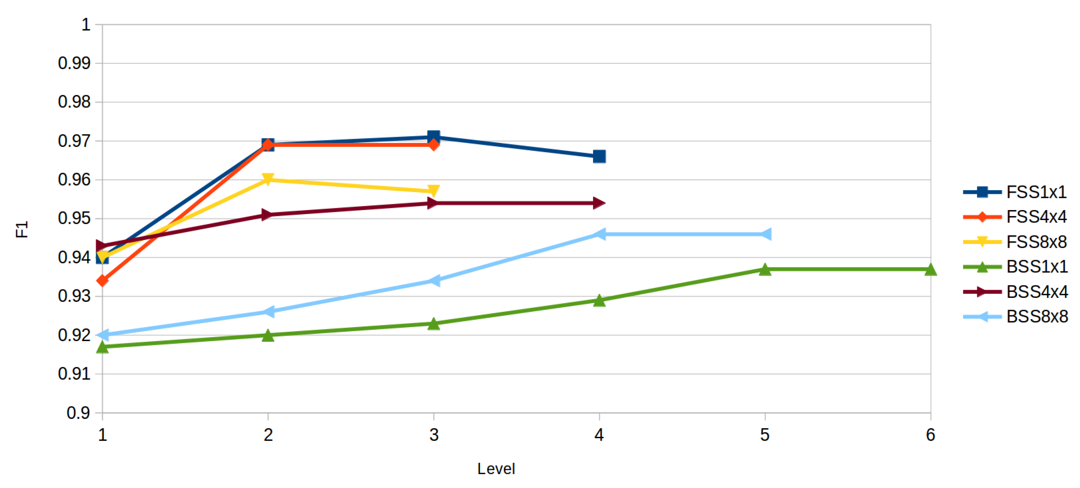
Figure 7 shows a comparative of the highest scores of each iteration of the different selection techniques. The maximum of each technique is obtained in the previous to the last level.

On general, Forward Subset Selection achieves better results than Backward Subset Selection. Backward selection computation time is higher than forward so is preferable to use a forward selection since computation time is shorter and the performance is better.

We have compared our method with two known CNN methods: Xception [41] and Siamese [42]. Xception is a Deep learning network inspired by Inception [43], where Inception modules, treated as intermediate step in-between regular convolutions, are replaced by depthwise separable convolutions. Siamese network, instead, is a Convolutional network that inputs two images and classifies if the two images are the same object. One of its advantages is that it gives good results even with small datasets.

Table 7. Comparison between standard DL methods and our proposal.

Method	F1
Xception	0.35
Siamese	0.89
Our proposal (FSS$1\times 1$)	0.97

shows a comparison between the proposed method and the two previous described methods. In the case of the Xception, the results are not as good as Siamese or our proposal as Xception works better for large datasets. Even if Siamese works better than Xception, it does not give better results than our proposal.

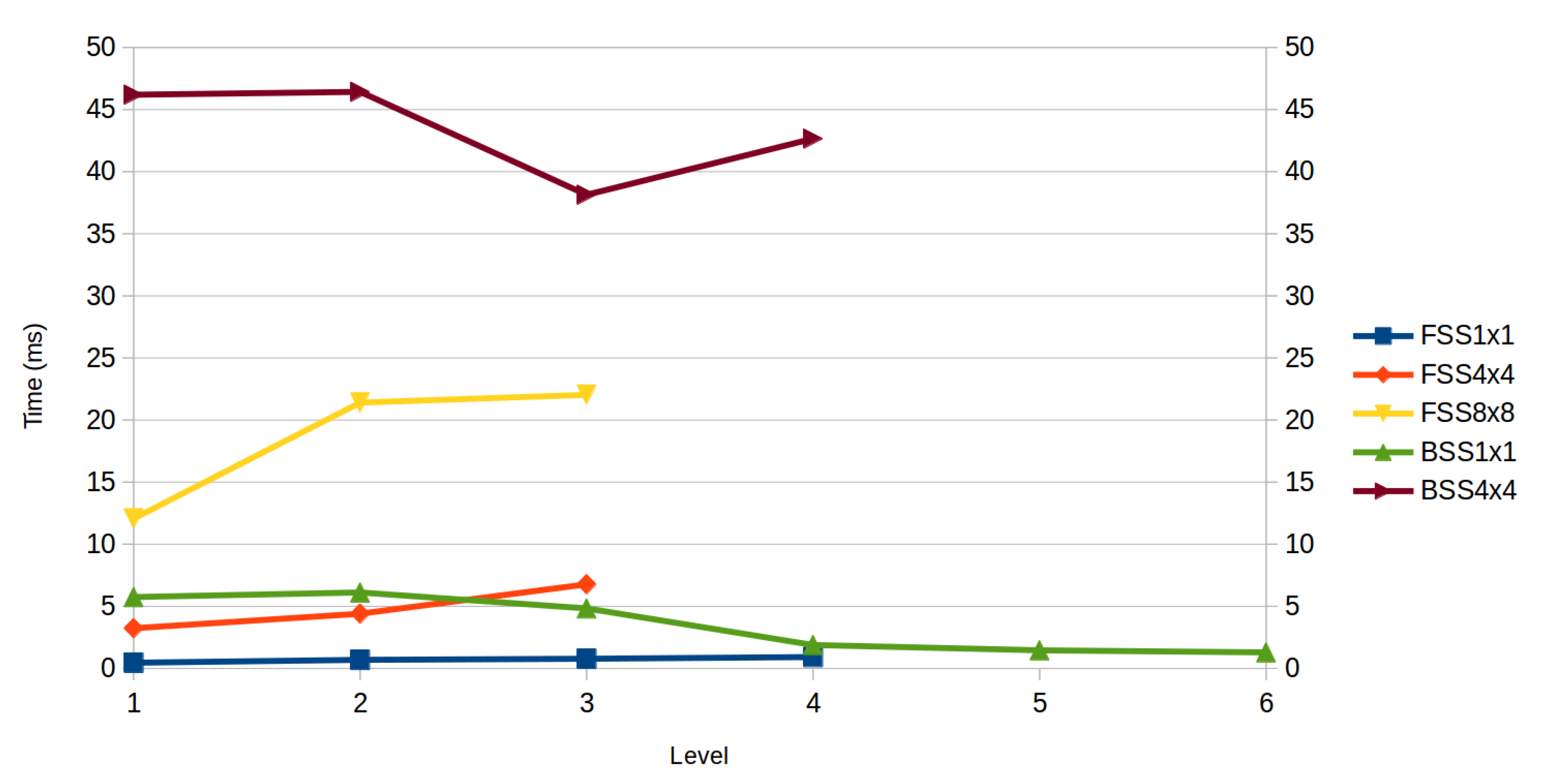
In terms of speed, Figure 8 shows a comparative of the test time for each of the methods. The time shown is the average of the different descriptors and classification techniques for testing one image. FSS$1\times 1$, FSS$4\times 4$, and BSS$1\times 1$ have a low computation time, and BSS$8\times 8$ version performs much slower than the rest of versions due to the high dimensionallity of the data.

Taking into account the speed and score the best option is to use FSS$1\times 1$. Although score is similar to the rest of the versions, it outperforms remaining in terms of speed.

5. Conclusions

The main two problems we have to deal with in computer vision in an industrial context is the complexity of the objects, that is, their unusual shape and texture-less objects, and the lack of large datasets to train CNNs that can handle the previous problem. To manage this situation, we proposed in this paper an approach for selecting the best combination of descriptor that, together, provides a better classification. Even if more than one descriptors has to been calculated, this method is still fast enough for real-time applications.

The proposed method is a greedy approach that iteratively adds (Forward Subset Selection) or removes (Backward Subset Selection) descriptors to the solution until performance is not improved. The resulting descriptor set always improves the quality of the classification comparing to the best descriptor by its own. This selection techniques can be extended to different datasets and contexts as proved within this paper and previous ones [34,35,36].

The used dataset for the experiments is composed by seven typical industrial texture-less objects. The proposed method achieves a state-of-the-art classification quality for that given dataset. Our method achieves a F1 of 0.971, 3% more than the best descriptor alone. Description and classification of a new image can be achieved in real-time applications, given its low processing time (between 10 and 50 ms).

The next steps will include a larger set of descriptors and DL networks in order to mix both classical and Neural Network methods. As this particular application is within a bigger industry 4.0 set-up, the following works will include not only a visual approach, but the application as a whole.

References

- Teichmann, M.; Weber, M.; Zoellner, M.; Cipolla, R.; Urtasun, R. MultiNet: Real-time Joint Semantic Reasoning for Autonomous Driving. arXiv 2016, arXiv:cs.CV/1612.07695. [Google Scholar]
- Ronneberger, O.; Fischer, P.; Brox, T. U-Net: Convolutional Networks for Biomedical Image Segmentation. arXiv 2015, arXiv:cs.CV/1505.04597. [Google Scholar]
- Yan, M.; Zhao, M.; Xu, Z.; Zhang, Q.; Wang, G.; Su, Z. VarGFaceNet: An Efficient Variable Group Convolutional Neural Network for Lightweight Face Recognition. arXiv 2019, arXiv:cs.CV/1910.04985. [Google Scholar]
- Liu, Y.; Wang, Y.; Wang, S.; Liang, T.; Zhao, Q.; Tang, Z.; Ling, H. CBNet: A Novel Composite Backbone Network Architecture for Object Detection. arXiv 2019, arXiv:cs.CV/1909.03625. [Google Scholar]
- Yuan, Y.; Chen, X.; Wang, J. Object-Contextual Representations for Semantic Segmentation. arXiv 2019, arXiv:cs.CV/1909.11065. [Google Scholar]
- Gómez, A.; de la Fuente, D.C.; García, N.; Rosillo, R.; Puche, J. A vision of industry 4.0 from an artificial intelligence point of view. In Proceedings of the 18th International Conference on Artificial Intelligence, Varna, Bulgaria, 25–28 July 2016; p. 407. [Google Scholar]
- Chen, C.; Liu, M.Y.; Tuzel, O.; Xiao, J. R-CNN for Small Object Detection. In Computer Vision—ACCV 2016; Lai, S.H., Lepetit, V., Nishino, K., Sato, Y., Eds.; Springer International Publishing: Cham, Switzerland, 2017; pp. 214–230. [Google Scholar]
- Xie, Q.; Luong, M.T.; Hovy, E.; Le, Q.V. Self-training with Noisy Student improves ImageNet classification. arXiv 2020, arXiv:1911.04252. [Google Scholar]
- Cubuk, E.D.; Zoph, B.; Mane, D.; Vasudevan, V.; Le, Q.V. AutoAugment: Learning Augmentation Policies from Data. arXiv 2019, arXiv:1805.09501. [Google Scholar]
- Kolesnikov, A.; Beyer, L.; Zhai, X.; Puigcerver, J.; Yung, J.; Gelly, S.; Houlsby, N. Large Scale Learning of General Visual Representations for Transfer. arXiv 2019, arXiv:1912.11370. [Google Scholar]
- Wang, J.; Chen, Y.; Yu, H.; Huang, M.; Yang, Q. Easy Transfer Learning By Exploiting Intra-domain Structures. arXiv 2019, arXiv:cs.LG/1904.01376. [Google Scholar]
- Nannia, L.; Ghidonia, S.; Brahnamb, S.; Le, Q.V. Handcrafted vs. non-handcrafted features for computer vision classification. Pattern Recognit. 2017, 71, 158–172. [Google Scholar]
- Lowe, D.G. Object recognition from local scale-invariant features. In Proceedings of the Seventh IEEE International Conference on Computer Vision, Kerkyra, Greece, 20–27 September 1999; Volume 2, pp. 1150–1157. [Google Scholar]
- Bay, H.; Tuytelaars, T.; Van Gool, L. SURF: Speeded Up Robust Features. In Proceedings of the European Conference on Computer Vision, Graz, Austria, 7–13 May 2006; pp. 404–417. [Google Scholar]
- Ojala, T.; Pietikäinen, M.; Harwood, D. A comparative study of texture measures with classification based on featured distributions. Pattern Recognit. 1996, 29, 51–59. [Google Scholar] [CrossRef]
- Fernández, A.; Álvarez, M.X.; Bianconi, F. Texture Description Through Histograms of Equivalent Patterns. J. Math. Imaging Vis. 2013, 45, 76–102. [Google Scholar] [CrossRef] [Green Version]
- Merino, I.; Azpiazu, J.; Remazeilles, A.; Sierra, B. 2D Features-based Detector and Descriptor Selection System for Hierarchical Recognition of Industrial Parts. IJAIA 2019, 10, 1–13. [Google Scholar] [CrossRef]
- Haralick, R.M.; Shanmugam, K.; Dinstein, I. Textural Features for Image Classification. IEEE Trans. Syst. Man Cybern. 1973, SMC-3, 610–621. [Google Scholar] [CrossRef] [Green Version]
- Wang, L.; He, D.C. Texture classification using texture spectrum. Pattern Recognit. 1990, 23, 905–910. [Google Scholar]
- Madrid-Cuevas, F.J.; Medina, R.; Prieto, M.; Fernández, N.L.; Carmona, A. Simplified Texture Unit: A New Descriptor of the Local Texture in Gray-Level Images. In Pattern Recognition and Image Analysis; Springer: Berlin/Heidelberg, Germany, 2003; Volume 2652, pp. 470–477. [Google Scholar]
- Xu, B.; Gong, P.; Seto, E.; Spear, R. Comparison of Gray-Level Reduction and Different Texture Spectrum Encoding Methods for Land-Use Classification Using a Panchromatic Ikonos Image. Photogramm. Eng. Remote Sens. 2003, 69, 529–536. [Google Scholar]
- Zhang, W.; Shan, S.; Gao, W.; Chen, X.; Zhang, H. Local Gabor binary pattern histogram sequence (LGBPHS): A novel non-statistical model for face representation and recognition. In Proceedings of the Tenth IEEE International Conference on Computer Vision (ICCV’05) Volume 1, Beijing, China, 17–21 October 2005; Volume 1, pp. 786–791. [Google Scholar]
- Tan, X.; Triggs, W. Enhanced local texture feature sets for face recognition under difficult lighting conditions. IEEE Trans. Image Process. 2010, 19, 1635–1650. [Google Scholar]
- Fernández, A.; Álvarez, M.X.; Bianconi, F. Image classification with binary gradient contours. Opt. Lasers Eng. 2011, 49, 1177–1184. [Google Scholar]
- Hussain, S.U.; Napoléon, T.; Jurie, F. Face Recognition using Local Quantized Patterns. In Procedings of the British Machine Vision Conference 2012; British Machine Vision Association: Guildford, UK, 2012; pp. 99.1–99.11. [Google Scholar]
- Chen, J.; Shan, S.; He, C.; Zhao, G.; Pietikainen, M.; Chen, X.; Gao, W. WLD: A Robust Local Image Descriptor. IEEE Trans. Pattern Anal. Mach. Intell. 2010, 32, 1705–1720. [Google Scholar] [CrossRef]
- Dalal, N.; Triggs, B. Histograms of oriented gradients for human detection. In Proceedings of the 2005 IEEE Computer Society Conference on Computer Vision and Pattern Recognition (CVPR’05), San Diego, CA, USA, 20–25 June 2005; IEEE: Piscataway, NJ, USA, 2005; Volume 1, pp. 886–893. [Google Scholar]
- Cover, T.; Hart, P. Nearest neighbor pattern classification. IEEE Trans. Inf. Theory 1967, 13, 21–27. [Google Scholar]
- Rish, I. An empirical study of the naive Bayes classifier. In IJCAI 2001 Workshop on Empirical Methods in Artificial Intelligence; IBM: New York, NY, USA, 2001; Volume 3, pp. 41–46. [Google Scholar]
- Breiman, L. Random forests. Mach. Learn. 2001, 45, 5–32. [Google Scholar] [CrossRef] [Green Version]
- Cortes, C.; Vapnik, V. Support-vector networks. Mach. Learn. 1995, 20, 273–297. [Google Scholar] [CrossRef]
- Lira, M.M.S.; de Aquino, R.R.B.; Ferreira, A.A.; Carvalho, M.A.; Neto, O.N.; Santos, G.S.M. Combining Multiple Artificial Neural Networks Using Random Committee to Decide upon Electrical Disturbance Classification. In Proceedings of the 2007 International Joint Conference on Neural Networks, Orlando, FL, USA, 12–17 August 2007; pp. 2863–2868. [Google Scholar]
- Breiman, L. Bagging predictors. Mach. Learn. 1996, 24, 123–140. [Google Scholar] [CrossRef] [Green Version]
- Shahlaei, M. Descriptor Selection Methods in Quantitative Structure–Activity Relationship Studies: A Review Study. Chem. Rev. 2013, 113, 8093–8103. [Google Scholar] [CrossRef] [PubMed]
- Rasines, I.; Remazeilles, A.; Bengoa, P.M.I. Feature selection for hand pose recognition in human-robot object exchange scenario. In Proceedings of the 2014 IEEE Emerging Technology and Factory Automation (ETFA), Barcelona, Spain, 16–19 September 2014; pp. 1–8. [Google Scholar]
- Molina, L.; Belanche, L.; Nebot, A. Feature selection algorithms: A survey and experimental evaluation. In Proceedings of the 2002 IEEE International Conference on Data Mining, Maebashi City, Japan, 9–12 December 2002; pp. 306–313. [Google Scholar] [CrossRef] [Green Version]
- Chinchor, N. MUC-4 Evaluation Metrics. In Proceedings of the 4th Conference on Message Understanding; Association for Computational Linguistics: Stroudsburg, PA, USA, 1992; pp. 22–29. [Google Scholar] [CrossRef] [Green Version]
- Forman, G.; Scholz, M. Apples-to-Apples in Cross-Validation Studies: Pitfalls in Classifier Performance Measurement. SIGKDD Explor. Newsl. 2010, 12, 49–57. [Google Scholar] [CrossRef]
- Platt, J.C. Sequential Minimal Optimization: A Fast Algorithm for Training Support Vector Machines; MIT Press: Cambridge, MA, USA, 1998. [Google Scholar]
- Robbins, H.; Monro, S. A Stochastic Approximation Method. Ann. Math. Statist. 1951, 22, 400–407. [Google Scholar] [CrossRef]
- Chollet, F. Xception: Deep Learning With Depthwise Separable Convolutions. In Proceedings of the 2009 IEEE Conference on Computer Vision and Pattern Recognition, Miami, FL, USA, 20–25 June 2009; pp. 248–255. [Google Scholar]
- Melekhov, I.; Kannala, J.; Rahtu, E. Siamese network features for image matching. In Proceedings of the 2016 23rd International Conference on Pattern Recognition (ICPR), Cancun, Mexico, 4–8 December 2016; IEEE: Piscataway, NJ, USA, 2016; pp. 378–383. [Google Scholar]
- Szegedy, C.; Vanhoucke, V.; Ioffe, S.; Shlens, J.; Wojna, Z. Rethinking the Inception Architecture for Computer Vision. In Proceedings of the IEEE Conference on Computer Vision and Pattern Recognition, Las Vegas, NV, USA, 26 June–1 July 2016; pp. 2818–2826. [Google Scholar]
Figure 1.
Random Forest example where each tree classifies the new instance and the resulting class is decided by majority voting.
Figure 2.
Support vector machine: maximum separation between two classes.
Figure 3.
Classification of a new image given a descriptor and a classifier.
Figure 4.
Full pipeline of the proposed method, including training, validation, and evaluation.
Figure 5.
Pictures of the parts used in the experiment.
Figure 6.
Histogram of all the used descriptors applied to a sample image. The vertical axis represents the number of occurrences of each texture unit normalized and the horizontal axis represents each of the texture units of the histograms. The descriptors are the ones that are part of D described at the beginning of Section 4.
Figure 7.
Comparative of highest F1 of each iteration of the Subset Selection techniques. FSS stands for Forward Subset Selection and BSS stands for Backward Subset Selection. The numbers after each selection technique stand for the number of windows the descriptor has been applied to.
Figure 8.
Times to classify an image with the different Subset selection methods on each level. The times on this Figure correspond to the average time that the classifier needs to classify an image using each descriptor on that level. The times of the BSS are not shown since its values are around 200 ms and distorts the plot.