Early Detection of Change by Applying Scale-Space Methodology to Hyperspectral Images

Abstract

Given an object of interest that evolves in time, one often wants to detect possible changes in its properties. The first changes may be small and occur in different scales and it may be crucial to detect them as early as possible. Examples include identification of potentially malignant changes in skin moles or the gradual onset of food quality deterioration. Statistical scale-space methodologies can be very useful in such situations since exploring the measurements in multiple resolutions can help identify even subtle changes. We extend a recently proposed scale-space methodology to a technique that successfully detects such small changes and at the same time keeps false alarms at a very low level. The potential of the novel methodology is first demonstrated with hyperspectral skin mole data artificially distorted to include a very small change. Our real data application considers hyperspectral images used for food quality detection. In these experiments the performance of the proposed method is either superior or on par with a standard approach such as principal component analysis.

1. Introduction

For a time-varying system, detection of unexpected or unwanted change in its evolution can be of paramount importance. Examples include environmental monitoring, process control, or, referring to the examples considered in this article, identification of potentially malignant changes in skin moles or the onset of food quality deterioration (see, for example, [1,2,3,4]). The first changes may be small and manifest themselves in different scales and it may be crucial to detect them as early as possible. Statistical scale-space methodologies (see Section 2) can be very useful in such situations since exploring the measurements in multiple resolutions can help identify subtle changes. Examples of scale-space methods designed for change detection are the SiNos technique for capturing non-stationarities in a time series [5] and the iBSiZer method for detecting changes in images [6]. Our goal was to develop a method that can detect minor change while at the same time keeping the number of false alarms to a minimum. This is important in practical applications as a successful method must have both high sensitivity and high specificity.

Recently, Hindberg et al. proposed a scale-space method for testing whether k multivariate data sets of same dimension originate from the same distribution [7]. Thus, the proposed method solves the classical k-sample problem using scale-space analysis and the method has proven successful in many applications. In the applications considered here the observed data consist of multivariate vectors obtained from spectral signatures and therefore changes in their characteristics can also be analyzed with this method. Unfortunately, it turns out that in this context the method suffers from two serious shortcomings: failing to detect very small changes and producing unacceptably high rates of false alarms in some situations (see Section 4). Our goal therefore is to design a scale-space method that would suffer less from these shortcomings.

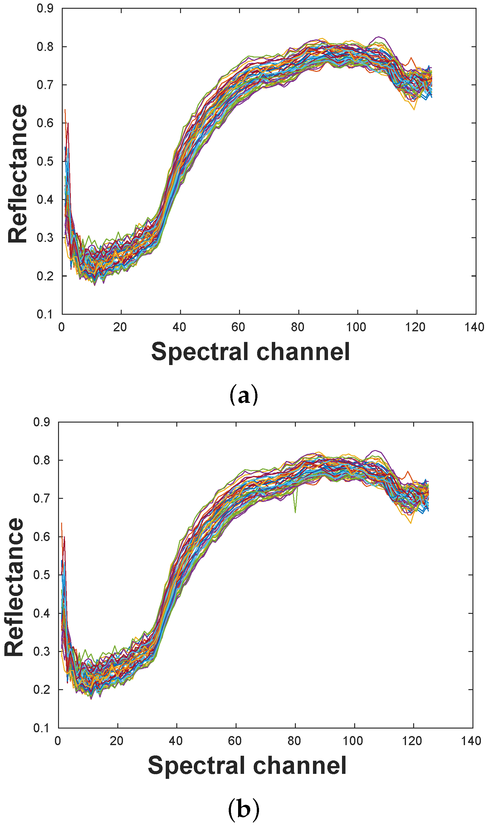
As an illustration of the difficulty of detecting very small changes, consider the example in Figure 1 which is discussed in more detail in Section 2 and Section 4. The original data set consists of a number of spectral signatures acquired by a push-broom hyperspectral camera, each signature corresponding to a particular spot in a skin mole. 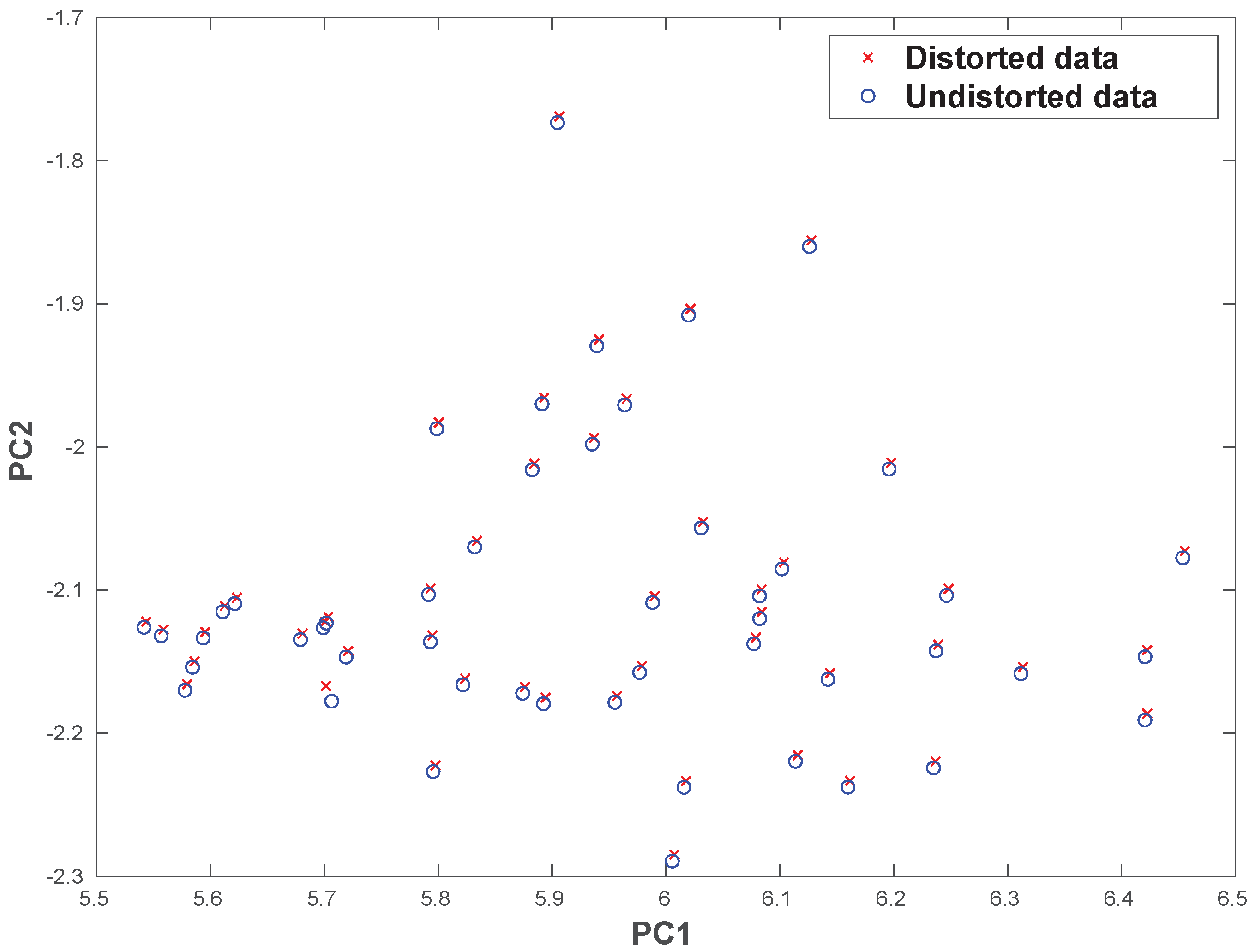Several acquisitions of the mole are taken at the same time, and an example of one acquisition is given in Figure 1a where each curve corresponds to a specific spectral signature. To simulate a situation where the mole might begin to turn malignant, we manually distorted just one spectral signature (thus corresponding to a very small local change in the mole) in another acquisition of the same mole at spectral channel 80 on the horizontal axis in Figure 1a. In case of real moles, the first changes may be extremely hard to detect and a method with high sensitivity and specificity is therefore crucial. In our test, the distorted set of signatures in Figure 1b was compared with 14 other acquisitions and the goal was to detect the small change we manually introduced. It turned out that such a small change is indeed detected by our new methodology but not by the method suggested in [7] nor by a standard approach such as principal components analysis (PCA). We will return in more detail to this example in Section 4.

2. Scale-Space Methodology

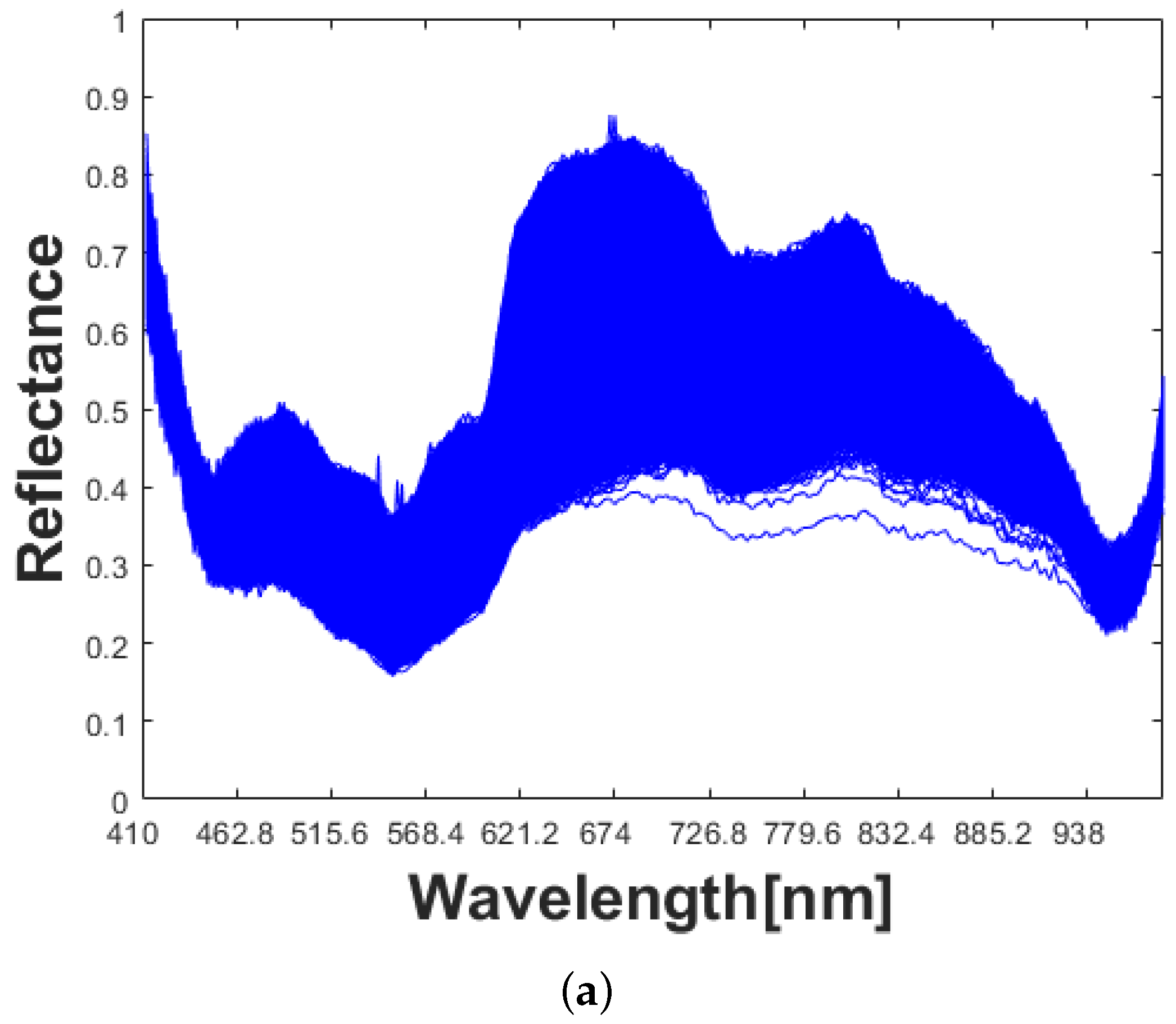
Scale-space theory is a framework for representing signals on multiple scales, developed by the computer vision, image processing and signal processing communities [8]. A recent review of statistical scale-space methodology can be found in [9]. The goal of statistical scale-space methodology is to extract statistically significant features from noisy data at several scales, often corresponding to different levels of resolution in the underlying object of interest. The data could be a set of observed curves where features at different levels of resolution might be of interest. These curves could, for example, correspond to spectral signatures from fish being frozen for different numbers of days, as is the case in our real data application. One acquisition of data consists of a number of p-dimensional vectors with unknown distribution, each vector representing the spectral signature at a particular pixel in the hyperspectral image. Thus, in our application, p represents the number of frequency bands (spectral channels) in the spectral signatures. In Section 4.2 we analyze three different acquisitions from the frozen fish. Under the null hypothesis, the number of days is assumed the same and the distributions are therefore assumed identical. In our approach, we perform several tests to flag when a new acquisition differs significantly from several previous acquisitions of day 0. The outcome of the tests is presented as a scale-space map, described in more detail below.

The core method of this paper is to test simultaneously for many different scales and positions (frequency bands). The scale s equals the number of different frequency bands being summed across. To be specific, this means that scale $s=1$ corresponds to the situation where we test if the observed values at spectral frequency d are different between acquisitions of spectral signatures. At scale $s=3$ and position d, a smoothing in terms of a weighted average of the observed values for spectral frequencies $d-1$, d and $d+1$ are used to test whether the acquisitions are different. The weights are calculated from an Epanechnikov kernel function (i.e., parabolic function) [10], the same as in [7]. For other scales, completely analogous smoothing over the frequency bands are made and used to perform the tests. Note that by applying this smoothing, we are able to test for differences in the acquisitions at all locations for a large number of scales. In fact, the tests are performed at all p spectral frequencies for a total number of $n_s$ different scales. Instead of looking at a single location or a single scale, the described scale-space approach can help detect changes that appear at several levels of smoothing, i.e., resolution.

However, when testing for differences between spectral signature curves in different acquisitions it can be difficult to select the critical rejection thresholds due to multiple testing. One possibility is to use the Bonferroni correction method [11] designed to reduce false positives in testing multiple hypotheses. As an alternative, we also tried the statistical inference method described in [12] to find suitable critical rejection thresholds for the scale-space map. The critical values are used to test if a new acquisition differs from the existing acquisitions.

The training procedure at a location $(d,s)$ is accomplished by comparing one acquisition to the others. To simplify the description we illustrate the methodology by testing for change in the sample mean, $\overline{X}$, over the pixels in the image. This training-procedure is the core difference between the method presented here and in [7], where there is a more direct comparison between curve families. Also, instead of the non-parametric Andersson-Darling test combined with either Bonferroni or False Discovery Rate correction for multiple hypothesis testing employed in [7], our novel method uses the t-test either with a Bonferroni correction or the inference approach suggested in [12]. Here, further, we assume that

$${\overline{X}}_1\sim N({\mu }_1,{\sigma }^2)$$

(1)

for acquisition one and

$$\overline{X}=\frac{1}{n-1}\sum _{k=2}^n{\overline{X}}_k\sim N\left(\mu ,\frac{{\sigma }^2}{n-1}\right),$$

(2)

for the remaining $n-1$ of the acquisitions. Here n is the total number of acquisitions. The normal assumption makes sense due to the central limit theorem since all ${\overline{X}}_k$’s, $k=1,\dots ,n$ are averages over a large number of observations. Note that this means that we perform the training procedure by leaving one out cross validation. In the description above, the mean is chosen as parameter, but we have also implemented and performed our testing procedure for the median, the standard deviation and the range. We do this since these parameters can better describe certain aspects of a distribution and may therefore capture different types of changes. In practice, we will therefore typically test all these parameters for potential changes. For parameters other than the mean, Equation (1) will be an approximation that may be violated in practice. Equation (2) will, however, still be a reasonable approximation for all parameters due to the central limit theorem, but will sometimes only hold approximately.

In our description below, we estimate ${\sigma }^2$ by the standard estimator for variance using all acquisitions apart from the one left out. In the case acquisition 1 is left out, this means that ${\sigma }^2$ is estimated by

$$S^2=\frac{1}{n-2}\sum _{i=2}^n{({\overline{X}}_i-\overline{X})}^2.$$

The critical quantile at location $(d,s)$, when only using the Bonferroni correction, is then given by

$$c(d,s)=t_{\frac{\alpha }{2p},n-2},$$

(3)

where $\alpha =0.05$ is the significance-level and p the number of spectral channels of each spectral signature curve. In addition to the Bonferroni-corrected quantile in Equation (3), we tried here the so-called global quantile

$$c{(d,s)}_G={\mathsf{\Phi }}^{-1}\left({\left(1-\frac{\alpha }{2}\right)}^{\frac{1}{p{\sum }_{k=1}^{n_s}{\theta }_k}}\right),$$

(4)

proposed in [12]. Here $\mathsf{\Phi }$ is the normal cumulative distribution function and $n_s$ denotes the number of rows in the scale-space map. Moreover, ${\theta }_k$ is given by

$${\theta }_k=2\mathsf{\Phi }\left(\frac{\sqrt{3logp}}{2s_k}\right)-1,$$

where $s_k$ is the scale in row k. In the testing procedure, we test

$$H_0:{\mu }_1=\mu \mathrm{against}{H}_1:{\mu }_1\ne \mu$$

using the test statistic

$$T=\frac{{\overline{X}}_{\mathrm{test}}-{\overline{X}}_{\mathrm{train}}}{S\sqrt{1+\frac{1}{n-1}}},$$

where $H_0$ is rejected if

$${\left|T\right|>c(d,s)\mathrm{or}\left|T\right|>c(d,s)}_G.$$

The algorithm is summarized in Algorithm 1 where $Par$ is used to denote the parameter we are using in the tests.

The outcomes of the tests are graphically summarized in a scale-space map, where the horizontal and vertical axes correspond to spectral frequency bands and scales, respectively. Thus, at each location $(d,s)$ we perform a test and the outcome is shown as a colored pixel, with red (blue) indicating a significant (not significant) difference at the position d for scale s.

To illustrate the method, consider the example introduced in Figure 1. Figure 2 shows the scale-space map produced by the procedure described above. The parameter used in this analysis was the range as it best detected the small change manually introduced to the data. Note how the map indicates a significant feature only for the smallest scales around the spectral channel given at point 80 on the horizontal axis. This is expected since the change is small and only present at one particular spectral channel for a single signature.

Algorithm 1 The SS_CC algorithm:

1: Initialization: Acquisitions that are correct under null hypothesis and the test-acquisitions are loaded.  2:  3: procedure SS_CC_train()  4:  5:     Input: The loaded acquisitions that are correct under the null hypothesis.  6:  7:     Initialization: The significance level $\alpha$ is chosen.  8:  9:     for $i=1:n$ do 10: 11:         procedure Leave one out(k) 12: 13:               return index vector $\mathbf{v}$ without k 14: 15: 16:         $\widehat{Par}\left(X_k\right)\sim N\left(Par,{\sigma }^2\right)$ from each $(d,s)$ location. 17: 18:         for j in $\mathbf{v}$ do 19: 20:             $\widehat{Par}\left(X\right)\sim N\left(Par,\frac{{\sigma }^2}{n-1}\right)$ from each $(d,s)$ location. 21: 22: 23:     return $mean\left(\widehat{Par}\left(X\right)\right),S$ 24: 25: 26: procedure SS_CC_test() 27: 28:     Input: The new acquisitions. $c(d,s),c{(d,s)}_G,mean\left(\widehat{Par}\left(X\right)\right),S$ 29: 30:     Initialization: The significance level $\alpha$ is chosen. 31: 32:     $T\leftarrow \frac{X_{test}-mean\left(\widehat{Par}\left(X\right)\right)}{S\sqrt{1+\frac{1}{n-1}}}$ 33: 34:     return Significance matrix for scale-space map

3. Hyperspectral Acquisition System

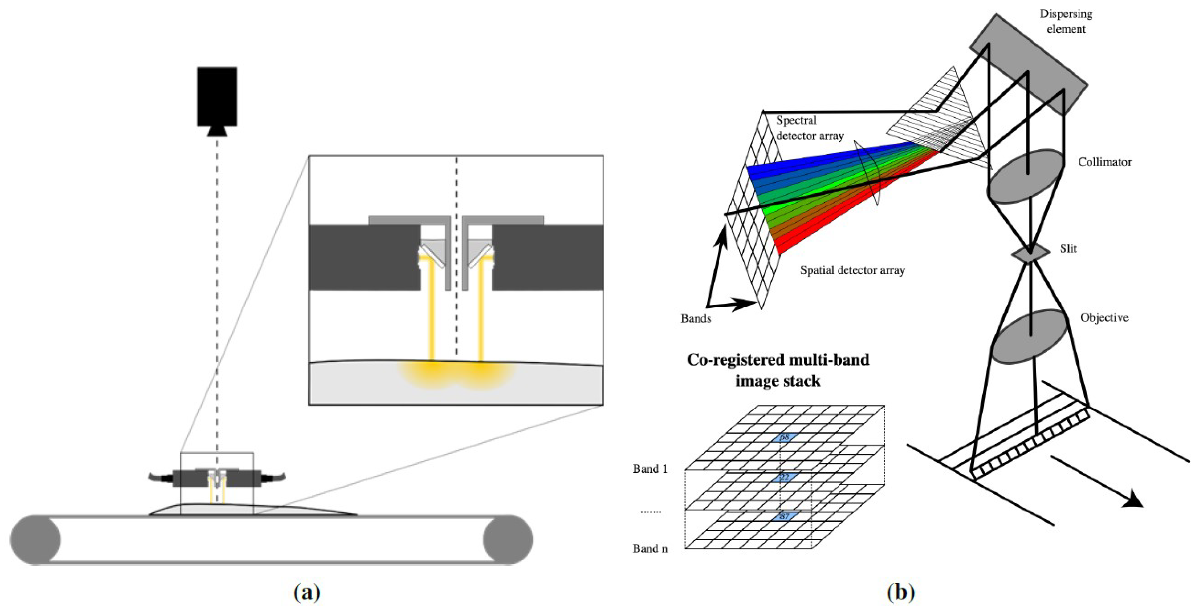
In order to capture spectral signature curves from fish, a customized hyperspectral imaging (HSI) acquisition system was employed. Image acquisition was performed with a push-broom hyperspectral camera with a spectral range of 410–1000 nm (see, for example, [3]) and spatial resolution of 0.3 mm across-track by 0.6 mm along-track (Norsk Elektro Optikk, model VNIR-1024). The camera was fitted with a lens focused at 1000 mm, mounted 1020 mm above a conveyor belt. Samples were illuminated using two custom made fiber optic line lights (Fiberoptics Technology inc., Pomfret, CT, USA), fitted with custom made collimating lenses yielding light lines approximately 5 mm wide (Optec S.P.A., Milano, Italy). Each line light was 400 mm wide, with six bundles of optical fibers. The light from 12 focused 150 W halogen lamps with aluminium reflectors (International Light Technologies, Peabody, MA, USA, model L1090) was fed into the fiberoptic bundles. The imaging and illumination setup is seen in Figure 3a. The optical power actually hitting the sample is approximately 0.16–0.79 Watt/(nm·sr·m${}^2$).

The illumination system is composed of a controller unit which allows controlling the brightness and the light source. This system permits us to regulate the light intensity according to the sample characteristics, such as color, size or other parameters dependent on light. The acquisition technique employed by this camera is the so-called push-broom method, which consists of an optical system capturing an image from a line in a plane as depicted in Figure 3b. The camera collects images as seen in Figure 3b.

To capture a hyperspectral image, either the camera or the sample must be moved synchronously with the shoot of the camera. In this case, the sample is moved using a linear actuator by a stepper motor along a line. The light used has been tested to emit in the whole spectral range. Before starting the capturing process, the camera must be focused and calibrated with a dark reference and a white reference. In this process, a tile with 99% of reflectance was chosen for the white reference.

The spectral signatures of the same frozen fish are taken on day 0, day 2, day 4, day 7 and day 10. On each day, we captured 912,082 signature curves in each of the four acquisitions made. The four acquisitions from day 0 were then compared to the other acquisitions in order to find significant differences as described in Section 4.

After image acquisition, the data from the reference images were used to perform a radiometric calibration of the raw spectral signature of each pixel of the HSI cube as suggested in [13].

$$CI=\frac{RI-DI}{WI-DI},$$

(5)

where $CI$ is the calibrated image, $RI$ is the raw image and $WI$ and $DI$ are the white and dark reference images, respectively.

4. Results

4.1. Artificial Mole Example

Recall from Section 1 that the data in our artificial data example were first obtained by acquiring a hyperspectral image of a skin mole and then modifying it manually in order to introduce a small distortion that could simulate a change in the mole itself. The HSI system used for the mole example differs from the one described in Section 3 and a detailed description can be found in [14]. In our analysis, we compared the proposed novel technique to the method of Hindberg et al. described in [7]. When applied in the present context, this method uses a two-sample test to decide if the test sample distribution differs from the distribution under the null hypothesis. We also experimented with principal component analysis (PCA, e.g., [15]). By examining the scatter plots of the most important principal component directions we concluded that PCA is unable to detect the distortion in the data as seen in Figure 4.

Because of this, we focus on a comparison between the new methodology and the one described in [7]. In general, the method in [7] performed poorly in this challenging situation. This was also reflected through the false positive rate (FPR) reported in Figure 5.

The FPR results obtained by the scale-space methodology for the range are quite impressive. However, it should be noted that we were not able to get similar results for the mean, the median or the standard deviation. This is to be expected because the range is clearly best suited for detecting the type of distortion we introduced to the mole data reported in Figure 1. Still, while the range is the natural parameter to use in this situation, it is also clear that range based inference can be very sensitive to outliers, should the data include them.

4.2. Freshness of Fish

As a real data example, hyperspectral signatures of frozen fish were analyzed. The data acquisitions took place on several different days after a fish was captured. In our analysis, a subset of ${301}^2$ = 90,601 signatures were analyzed in each acquisition. This is a subset of the full HSI cube that consists of 912,082 spectral signature curves, chosen due to the upper limit of 130 GB of RAM available in the computer used to perform our experiments. An example taken from one fish at day 0 is given in Figure 6a and signatures for two different acquisitions for the same fish at day 4 are given in Figure 6b,c, respectively. Comparison of the signatures of Figure 6a with Figure 6b,c results in the significance maps in Figure 7. There the four panels show the results using two different parameters, the mean and the median. Changes are detected with the mean and the median, but with the standard deviation and the range, no statistically significant changes were detected. A careful examination of the curves in Figure 6 reveals that location parameters are expected to detect changes best in this case and this is indeed what happens. Typical FPR results are reported in Figure 8. From the results here we see that the Hannig-Marron critical value gives better performance. The difference is, however, not very clear in this example.

Due to computational challenges, results for the method of Hindberg et al. in [7] and PCA could not be obtained for the full data sets. In comparisons using only smaller subsets of the data, all three methods performed similarly in detecting changes while the their FPRs were similar to Figure 8.

5. Discussion and Future Research Directions

The experimental results of Section 4.1 suggest that the proposed scale-space methodology can be successful in detecting small changes in a hyperspectral image. To be useful in practice, such a method must have both high sensitivity and high specificity and our results for the artificial mole data clearly show promise in this respect. We are currently in the process of acquiring a large number of HSI data sets related to skin moles and lesions in collaboration with several hospitals in the Canary Islands, Spain. Our long term goal is to design a successful classifier for such data and the preliminary results obtained so far are promising [14]. However, we believe that a system capable of monitoring dynamical changes in a mole will be even more important as it is likely to be the best way to detect severe skin cancer at an early stage. In the future, we will therefore work on the development of such a system and our ultimate goal is to design a decision support tool based on just a few frequency bands so that an affordable version could be implemented on a smart phone and thereby be available for use on an individual basis.

One aspect of hyperspectral image data not utilized in the present study is its spatial structure. Taking spatial information into account is important because it can significantly improve the interpretation of the data when changes have been detected. Spatial information can be used both in the development of the change detection algorithm and in the interpretation of the results. Besides mole monitoring applications, a successful change detection method incorporating spatial information could perhaps also be used in the analysis of brain fMRI data for the detection of early signs of, for example, Alzheimer’s disease [16].

Another area where the present methodology can be directly applied is in the design of robust controllers for Type 1 Diabetes patients. Successful results in this area are currently being obtained by using reinforcement learning (RL), see, for example, [17]. In the design of such machine learning algorithms, a good description of the patient’s state space is needed for the algorithm to be able to learn better strategies. The state space contains information used to describe the patient’s condition at a given time. Typically, the elements of state space in this context are time series of the most recent past blood glucose levels of the patient. At the beginning of the learning phase of an RL algorithm, the state space may be chosen reasonably coarse. During the learning process, the state space then may need to change because the algorithm encounters new states, that is, new glucose level time series, not included in the initial state space. The detection of such changes in the state space time series can be accomplished by the kind of methods discussed in this article. Research in this direction will therefore be pursued in the near future.

We also plan to further develop our approach to the analysis of fish freshness discussed in Section 4.2. For the design of a practical system that can be reliably used in fish industry one must first analyze data sets from several different fish at several time points after capturing. Then it is possible estimate both the within variance (of a day) and the between variances (between different time points) exhibited by the hyperspectral signatures. We will acquire such data in the future and the goal will be to perform an analysis that demonstrates how early changes in fish (or other types of food) quality can be detected in a reliable way.

Finally, we believe that the proposed methodology can be useful in combating problems in the so-called “$p>n$” problems now commonly found in statistical data analyses. Here p and n refer to the number of model parameters and the number of available observations, respectively, and such problems are very common in applications that involve high dimensional data, see e.g., [18,19]. The methodology developed in this article was partly motivated by the need to improve the technique of Hindberg et al. [7] which was originally designed exactly for the $p>n$ situation where common covariance matrix based multivariate methods such as PCA are useless. Being clearly an improvement of the technique of Hindberg et al., the method developed in this article is potentially useful in the analysis of such high dimensional data.

6. Concluding Remarks

We have developed a scale-space methodology that can successfully detect small changes in curve data. In addition, the developed methodology has the potential to produce few false alarms, an important feature for any detection method. We analyzed the performance of the proposed method on data with artificial and real changes. In addition, we compared the new method to some natural competitors and demonstrated that it at least in some cases outperforms them. Finally, we outlined several future research directions for the new methodology that can lead to important new findings.