Event Density Based Denoising Method for Dynamic Vision Sensor

Abstract

Dynamic vision sensor (DVS) is a new type of image sensor, which has application prospects in the fields of automobiles and robots. Dynamic vision sensors are very different from traditional image sensors in terms of pixel principle and output data. Background activity (BA) in the data will affect image quality, but there is currently no unified indicator to evaluate the image quality of event streams. This paper proposes a method to eliminate background activity, and proposes a method and performance index for evaluating filter performance: noise in real (NIR) and real in noise (RIN). The lower the value, the better the filter. This evaluation method does not require fixed pattern generation equipment, and can also evaluate filter performance using natural images. Through comparative experiments of the three filters, the comprehensive performance of the method in this paper is optimal. This method reduces the bandwidth required for DVS data transmission, reduces the computational cost of target extraction, and provides the possibility for the application of DVS in more fields.

1. Introduction

The rapid development of imaging sensors has caused a geometric increase in the image-data quantity, rendering it difficult for the current algorithms and computing power to process such massive image data rapidly. Dynamic vision sensor (DVS) can solve the problem of large image-data quantities, from a hardware perspective [1,2,3]. Dynamic vision sensors are biologically inspired event-based image sensors. In the case of fast moving targets and large dynamic range, DVS can achieve low power visual sensing, but it is a challenge to traditional detectors [4].

The pixel of DVS detects the change of light intensity. When the change reaches a certain threshold, the imaging system outputs the event coordinate, time stamp, event polarity or gray level information [5]. The output of events is asynchronous, rather than the synchronous output of traditional sensors in frame. Such characteristics make DVS more advantageous in areas such as moving target detection, simultaneous localization and mapping (SLAM), and drones [6,7,8,9,10,11,12,13]. At present, commercial companies have used them for automotive and other fields [14,15].

However, due to thermal noise and junction leakage current, there will be output even if there is no change in light intensity [16], called background activity (BA). It can affect the image quality, waste the communication bandwidth, and consume unnecessary computing power. Therefore, a DVS denoising algorithm is necessary.

Background activity differs from real events in that there is a higher spatiotemporal correlation between real events. In spatiotemporal images, the images of real events are denser, and BA is sparser. This difference can be used to denoise by judging the space-time density of events; the quality of the image can also be quantified by this property.

The imaging system used in this work is CeleX-IV from CelePixel Technology Co., Ltd. [3]. The resolution of the sensor is 768 × 640, an Opal Kelly XEM6310 control board drives sensors and outputs data, the maximum output rate is 200Meps, and each pixel occupies 18 × 18 μm² with a 9% fill factor. Unlike dynamic and active-pixel vision sensor (DAVIS), the event output by this sensor does not contain polarity information, but contains light intensity information of the event [17].

In this study, we present a method for reducing the noise in the event stream of a DVS, based on the event density in the spatiotemporal neighborhood. Our algorithm derives inspiration from the spatiotemporal principle and event-based optical flow [18,19]. This method has two steps. The first step filters out random noise and the second step filters out hot pixels. At the same time, a method for quantifying image quality is proposed based on the spatiotemporal correlation: model a piece of event data, use a two-dimensional Gaussian kernel to convolve with each event, determine the real event probability of the noise, and evaluate the amount of noise. This method can quantify the quality of natural images and filter performance. There is no need to design fixed image stimulation in [4]. This method can evaluate the filtering effect and image quality as long as there is an image, and it is easy to implement and reproduce.

The remainder of this paper is organized as follows: Section 2 reviews the related work on space-time correlation. Section 3 introduces the classification of noise, the concepts in the algorithm, and the design of the filter. Section 4 introduces methods for quantifying and evaluating image quality. Section 5 designs experiments to compare the denoising results of different filters. Section 6 discusses the experimental results and Section 7 presents the conclusions.

2. Materials and Methods

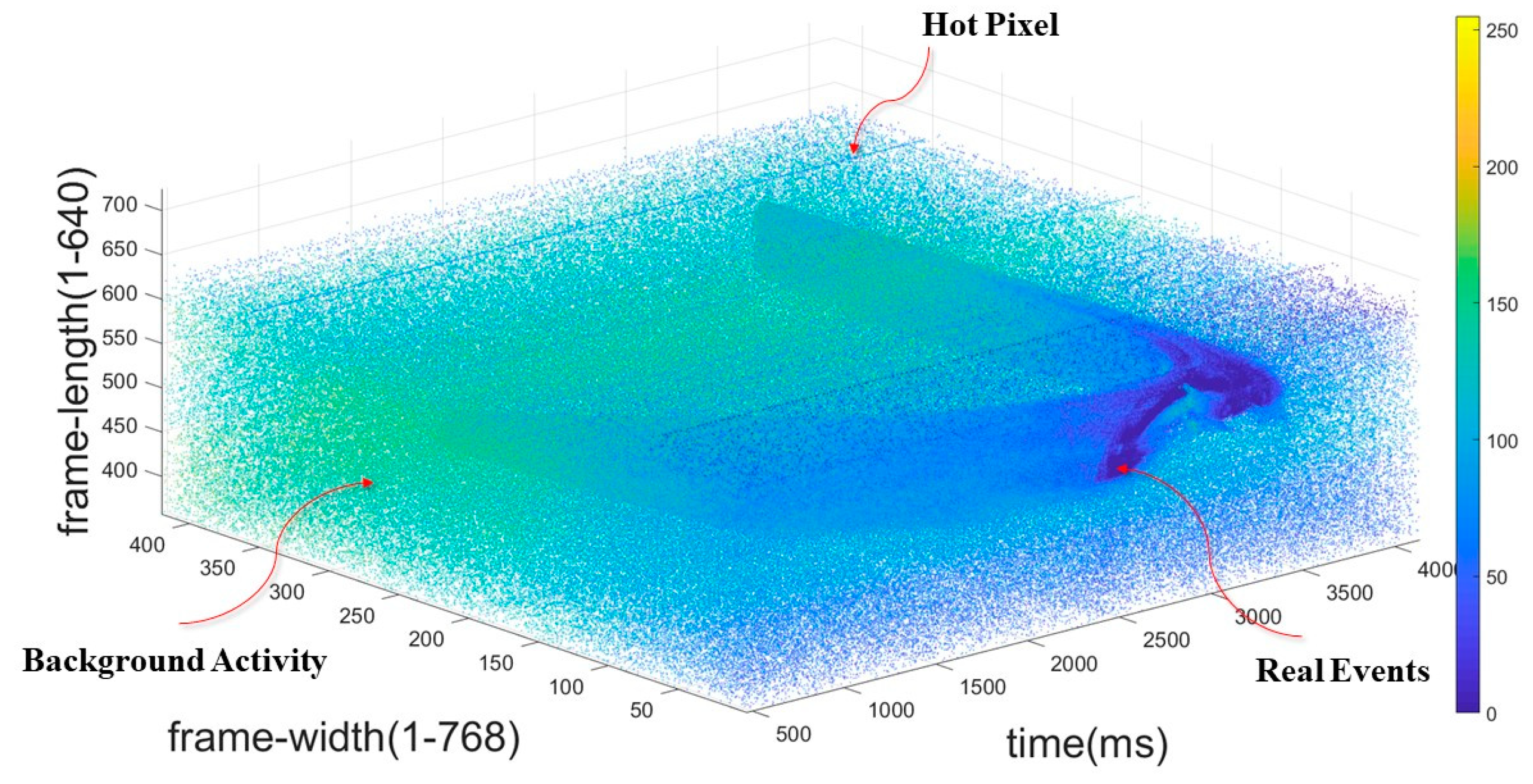
The background activity is caused by many factors such as charge injection, the leakage of the transistor section of the reset switch, and thermal noise. The location of the background activity is random and less frequent than real events. In addition, similar to the hot pixel of traditional image sensors, a similar situation exists in DVS. Because the pixel cannot be reset properly, the pixel continuously outputs events [20]. In the image, two kinds of noise exist at the same time. As shown in Figure 1, a filter is required to filter out these two kinds of events that should not occur.

Khodamoradi’s team has confirmed through testing that the BA events from the DVS can be assumed to be drawn from a Poisson distribution [21]. Calculating the probability that a single pixel will generate BA numbers within a finite time interval can be performed by the Poisson process:

$$\mathrm{P}\left\{\mathrm{N}\right(\mathrm{t})=\mathrm{n}\}=\frac{{(\lambda t)}^n}{n!}{e}^{-\lambda t}.$$

(1)

In Equation (1), t is the time interval, n is the number of BAs reached in the time interval, and λ is the average rate of each pixel BA.

It was found in previous research that the difference between BA and real events is that BA lacks correlation with other BAs in its spatiotemporal neighborhood. The spatiotemporal correlation of two events e₁ (x₁, y_1, t₁), e₂ (x₂, y₂, t₂) can be expressed as:

$$spatiotemporalcorrelation\iff \{\begin{array}{c}\left|x_1-x_2\right|\le dN\\ \left|y_1-y_2\right|\le dN\\ \left|t_1-t_2\right|\le dt\end{array}.$$

(2)

In Equation (2), dN is the spatial neighborhood size, and dt is the time neighborhood size. Based on this characteristic, many filtering methods are designed, and several related works are introduced below.

Delbruck proposed the background activity filter in [22]. This filter will filter out events that have no events in the surrounding 8 pixels in the past time T. Although BA is sparse compared to real events, there is a possibility for two BAs to be close enough in spatiotemporal neighborhood; in this case, the filter passes the latter BA.

Liu’s filter groups pixels by subsampling [18]; the subsampling factor is S, so S² pixels are a group. The filter determines the time correlation of events in this group, that is, determines whether the time difference between events is less than T; if, yes, passes, otherwise filter.

Khodamoradi’s filter uses a specific storage method to store the timestamps of events; two 32-bit storage units are used in every row and column to store the coordinates, polarity, and timestamp of the latest event. For example, event e₀ (x₀, y₀, t₀, p₀), y₀, p₀, t₀ are stored in the storage unit of x₀, x₀, p₀, t₀ are stored in the storage unit of y₀. This way saves storage space. However, this storage method can only recover events of up to 6 pixels, and more importantly, these 6 pixels are not necessarily neighboring pixels of the newly arrived event pixels. For example, the event sequence is e₁ (x, y, t₁, p), e₂ (x+2, y, t₂, p), e₃ (x, y+2, t₃, p), e₄ (x, y, t₄, p), where t₁ <t₂ <t₃ <t₄, and t₄ – t₁ < T. In this case, according to the coordinates of e₄, only the addresses of e₂ and e₃ can be recovered; e₄ is not adjacent to them and will be filtered. However, e₄ and e₁ have spatiotemporal correlation and should not be filtered. So this will lose more real events.

In the study of filter performance evaluation, Daniel Czech proposed a method of repeated recording using a fixed pattern to determine whether the event is noise or a real event, thereby evaluating the performance of the filter [4]. In this method, the events generated by each pixel are represented by a pulse function:

$$SF(x,y,p)={\mathsf{\Sigma }}_i\delta (t-t_0)0<i<n,x_i=x,y_i=y,p_i=p.$$

(3)

For each event, the convolution of the same-polarity event sequence with the one-dimensional Gaussian kernel is used to estimate the event probability of each point in the record, and then the average signal probability and total signal probability of the event stream before and after filtering are calculated as metrics to evaluate the filter performance. Compared with the traditional image-to-noise ratio method for evaluating filters, due to the requirements of a fixed image generator and other hardware environments, such an evaluation method has poor propagation. There is currently a need for a metric that can use natural images to evaluate event stream quality and filter performance.

3. Algorithm

3.1. Event Density and Event-Density Matrix

Before introducing the algorithm, we first define two concepts: the event density matrix and event density. The output event of a DVS can be represented by three parameters, e(x, y, t), which include the x and y coordinates of the image plane, where the event is located, and the timestamp, respectively. The timestamp is added to the output by the field programmable gate array (FPGA) driving the DVS. According to the spatiotemporal correlation principle, real events are related to events adjacent to each other in time and space; hence, a spatiotemporal neighborhood is set for each event, as shown in Figure 2. The red point indicates the newly arrived event at $t_1$, in the center of a spatial neighborhood sized $L\times L$; $L$ is odd, the time neighborhood is $(t_1-\mathsf{\Delta }t,t_1)$, and the spatiotemporal neighborhood is expressed as ${\mathsf{\Omega }}_{\mathsf{\Delta }t}^L$. The $L\times L$ pixel output events in ${\mathsf{\Omega }}_{\mathsf{\Delta }t}^L$ are respectively accumulated, and the result is placed in the corresponding position in an $L\times L$ sized matrix, which is the density matrix, $D$; the matrix element, $D_{i,j}$, is expressed as Equation (4),

$$D_{i,j}={\displaystyle \sum _{t=t_0-\mathsf{\Delta }t}^{t_0}\gamma (x_0-\frac{L-1}{2}-1+i,y_0-\frac{L-1}{2}-1+j,t)}1\le i,j\le L,$$

(4)

where $x_0,y_0$ are the spatial coordinates of the newly arrived event. $\gamma (x,y,t)$ is a binary function:

$$\gamma (x,y,t)=\{\begin{array}{l}1ifthereisanevente(x,y,t)\\ 0otherwise\end{array}.$$

(5)

After obtaining the density matrix, define the event density, $d$, as the L1 norm of the density matrix:

$$d={\Vert D\Vert }_1$$

(6)

3.2. Denoising Algorithm

Because the pixel structure and readout circuit of DVS are very different from traditional image sensors (CCD, CMOS), the output data form is completely different. The data of the frame image can be expressed mathematically as a matrix with the same size as the sensor pixels. The DVS event stream is asynchronous output, that is, when the pixels of the sensor are activated, the events generated by these pixels are output, and if they are not activated, they are not output. The data generated in this way is sparse and cannot form a matrix like a frame image.

In DVS, events are delivered in pulses, so, events can be expressed as pulse functions mathematically:

$$e_0(x_0,y_0,t_0)\Rightarrow \delta (x-x_0,y-y_0,t-t_0).$$

(7)

The DVS event steam can be expressed as the accumulation of event pulses, that is:

$$\mathrm{ES}(x,y,t)=\sum _{\mathrm{i}=1}^{\mathrm{N}}\delta (x-x_i,y-y_i,t-t_i),$$

(8)

where N is the number of events contained in the event stream and δ(x, y, t) is a pulse function.

The noise model Equation (1) shows that the more BAs generated by a non-hot pixel, the lower the probability within a fixed time interval. However, real events are generated by the movement of objects or the change in light intensity. The activated pixels are generally adjacent. According to the handshake circuit structure, it can be known that the event timestamps in the same row are the same, and the time difference between events in adjacent rows is in nanoseconds. Therefore, in a certain space-time, the number of BAs is less than a certain threshold with a high probability, and the number of events generated by the real target will be greater than this threshold, which can be expressed as:

$${\displaystyle \underset{x_i,y_i,t_i\in {\mathsf{\Omega }}_{\mathsf{\Delta }t}^L}{\iiint }\delta (x-x_i,y-y_i,t-t_i)}dxdydt\{\begin{array}{l}<\mathsf{\Psi }ifthereareBAsin{\mathsf{\Omega }}_{\mathsf{\Delta }t}^L\\ \ge \mathsf{\Psi }ifthereareObjectsin{\mathsf{\Omega }}_{\mathsf{\Delta }t}^L\end{array},$$

(9)

where Ψ is the threshold of the number of events. The threshold is related to the threshold of the ON or OFF comparator of the DVS and the size of target.

For the noise generated by the hot pixel, if there are BAs around the hot pixel, filtering based on the criteria supported by the events of the surrounding pixels will be affected. Therefore, the BA needs to be filtered out before the hot pixel is processed.

This algorithm is divided into two steps: the first step involves coarse filtering, where the random noise is filtered out, and the second step involves fine filtering, where the hot pixel is filtered. As the random-noise event density is lesser than that of the real event, the threshold of the event density is set to determine whether the event is noise. The event density, $d$, is first calculated in its spatiotemporal neighborhood, ${\mathsf{\Omega }}_{\mathsf{\Delta }t}^L$, for each input event, $e(x,y,t)$. If the event density is less than the threshold, Ψ, the event is random noise and is filtered out; if it is greater, the event is stored in the coarse filtering result, and enters fine filtering.

As a hot pixel appears at high frequency in a fixed position, it is difficult to filter using the event-density threshold alone; hence, the result of the coarse filtering is fine filtered. In the second step of filtering, the density matrix, $D$, is calculated for the coarse filtering result event in the spatiotemporal neighborhood, ${\mathsf{\Omega }}_{\mathsf{\Delta }t}^3$, of the new event. The flicker noise decision value, R, is then calculated:

$$R={\Vert \langle P,D\rangle \Vert }_1,$$

(10)

where

$$P=\left(\begin{array}{ccc}1& 1& 1\\ 1& 0& 1\\ 1& 1& 1\end{array}\right)$$

(11)

and $\langle •\rangle$ is the inner product. After coarse filtering, there are other real events in the small spatiotemporal neighborhood of the real event, but there is no other noise around the flicker noise, so the above calculation is performed on the density matrix. If R = 0, it is noise, otherwise it is retained as the result of the final noise reduction.

4. Evaluation Method

It is difficult to obtain target information from a single event in the event image of the DVS, and it is difficult to distinguish whether it is a real event or noise after imaging. When the trajectory of the target is known, the time correlation of events generated by a single pixel can be counted through repeated recording. The higher the correlation, the higher the probability of real events, and the lower the probability of noise. However, in natural scenes, the target’s motion information cannot be obtained, and relying on this method of judging image quality is not feasible.

According to the spatiotemporal correlation of events, the average time and space between real events is smaller than that of the noise. A single event contains very little information, and the probability that an event is a signal event or noise requires a period of event flow to calculate. First calculate the spatial distance between the event and other events, reduce the dimension of the parameter, and use the event e₀(x₀, y₀, t₀,) as the “center” to express the event sequence, that is

$$ES(d,t)={\displaystyle \sum _{i=1}^N\delta (d-\mathsf{\Delta }{d}_i,t-\mathsf{\Delta }{t}_i)},$$

(12)

where δ(d, t) is the pulse function, N is the number of events,

$$\mathsf{\Delta }{d}_i={\left[\left(x_i-x_0\right)+\left(y_i-y_0\right)\right]}^{\frac{1}{2}},\mathrm{and}$$

(13)

$$\mathsf{\Delta }{t}_i=\left|\left(t_i-t_0\right)\right|.$$

(14)

Then use a two-dimensional Gaussian kernel

$$G(d,t)=\frac{1}{2\pi {\sigma }_1{\sigma }_2}{e}^{-\frac{1}{2}(\frac{d^2}{{\sigma }_1^2}+\frac{t^2}{{\sigma }_2^2})}$$

(15)

to convolve with the above event sequence to get the real event probability of the event

$$P_{e_0}=ES(d,t)\otimes G(d,t),$$

(16)

namely

$$P_{e_0}={\displaystyle \sum _{i=1}^N\frac{1}{2\pi {\sigma }_1{\sigma }_2}{e}^{-\frac{1}{2}(\frac{{(\mathsf{\Delta }{d}_i)}^2}{{\sigma }_1^2}+\frac{{(\mathsf{\Delta }{t}_i)}^2}{{\sigma }_2^2})}}.$$

(17)

Among them, σ₁ and σ₂ are the standard deviations of the spatial distance d and the time distance t, respectively, which are determined by the resolution of the DVS and the time interval of the event stream. The location and time of the event are independent of each other, so $\rho =0$ in the normal distribution.

It can be seen from the formula that if there is only one hot pixel noise in the image, then the real event probability of these noises will be abnormally high. In order to eliminate this effect, the real event probability when d = 0 is set artificially as 0, namely

$$P_{e_0}=\{\begin{array}{cc}{\displaystyle \sum _{i=1}^N\frac{1}{2\pi {\sigma }_1{\sigma }_2}{e}^{-\frac{1}{2}(\frac{{(\mathsf{\Delta }{d}_i)}^2}{{\sigma }_1^2}+\frac{{(\mathsf{\Delta }{t}_i)}^2}{{\sigma }_2^2})}}& d\ne 0\hfill \\ 0& d=0\hfill \end{array}.$$

(18)

For the evaluation of image quality, it is necessary to calculate the number of events with low real events probability in the image. The criterion for low real events probability is less than or equal to BAs’ average real events probability. BA will change with factors such as light intensity, ON/OFF threshold, sensor temperature, etc. Therefore, the selection of BA is performed by manually opening the window in the original event stream, that is, selecting some pixels in the area without target movement, counting the real event probability of each BA, and then calculating the average real event probability of the BA, P_ARE. Comparing the passed events with it, the fewer events less than the BAs’ average real event probability, namely noise in real (NIR), the less residual noise after filtering. NIR is calculated from Equation (19), namely

$$NIR={\displaystyle \sum \delta (x-x_i,y-y_i,t-t_i)}{e}_i(x_i,y_i,t_i)\in {\mathsf{\Lambda }}_{PE}and{P}_{e_i}\le P_{ARE},$$

(19)

where Λ_PE is a collection of passed events in the period. Comparing the filtered noise events with it, the fewer events higher than the BA average true event probability, namely real in noise (RIN), the fewer the filtered real events. RIN is calculated from Equation (20), namely

$$RIN={\displaystyle \sum \delta (x-x_i,y-y_i,t-t_i)}{e}_i(x_i,y_i,t_i)\in {\mathsf{\Lambda }}_{FE}and{P}_{e_i}>P_{ARE},$$

(20)

where Λ_FE is a collection of filtered events in the period.

5. Experiment and Evaluation

In this section, we will use the data collected by DVS to compare the performance of the filters. The filters to be compared are Delbruck’s filter, Liu’s filter, and Khodamoradi’s filter. All algorithms were implemented using MATLAB. The data used was collected by the CeleX-IV imaging system. The imaging target was a swaying ball in natural light.

In the experiment, the parameters used in the method of this paper are L = 5, dt = 5 ms, and the threshold is 3. In the control experiment, setup was done according to the frequency of BA in CeleX-IV and the time window used by Delbruck’s filter. Khodamoradi’s filter is set to 1 ms, and the downsampling factors of Liu’s filter are 1, 2, namely time stamps from 2 × 2 and 4 × 4 pixels are stored in a cell respectively, and the time window is 1 ms.

The event stream is sorted in chronological order, and the events are sent to the filter sequentially. After filtering, the passed events and filtered events are saved separately to evaluate the performance of the filter, and they are judged by the amount of noise in the passed events and the number of real events in the filtered events in the same time period. The lower the values, the better the filter performance.

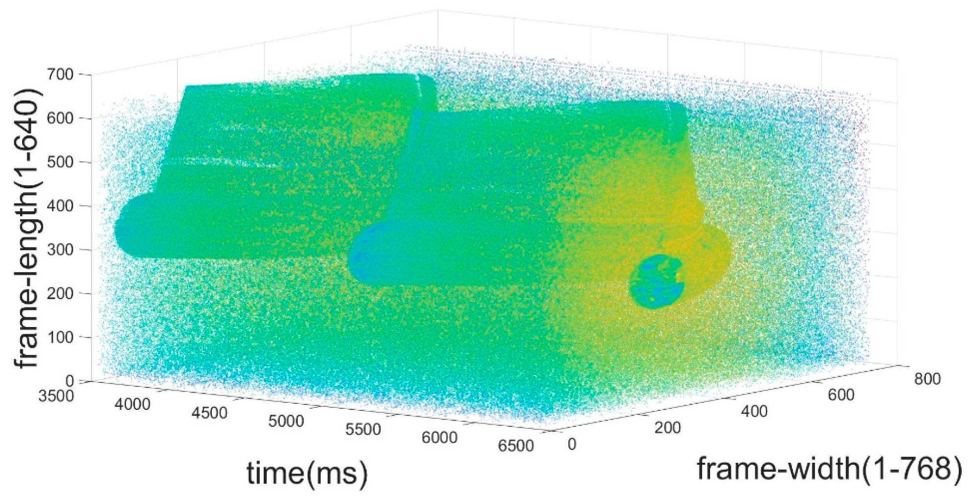
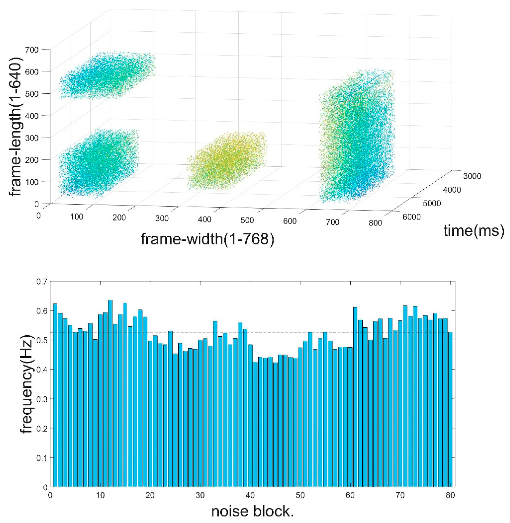
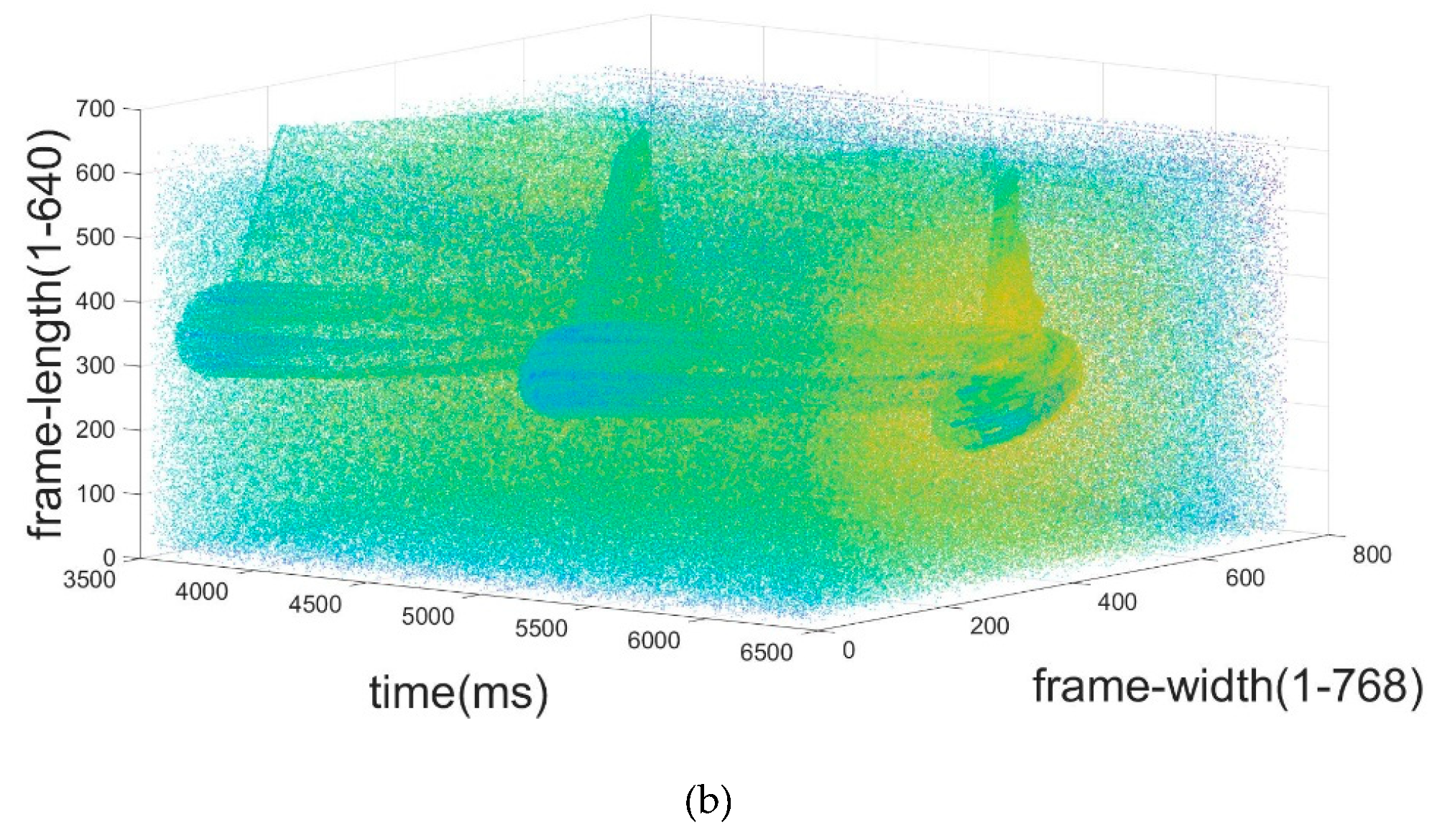
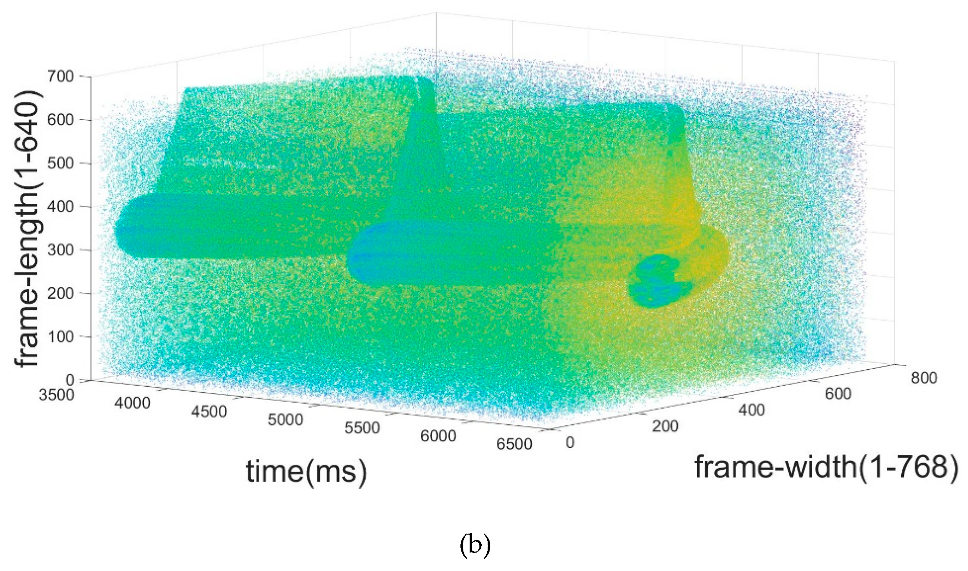
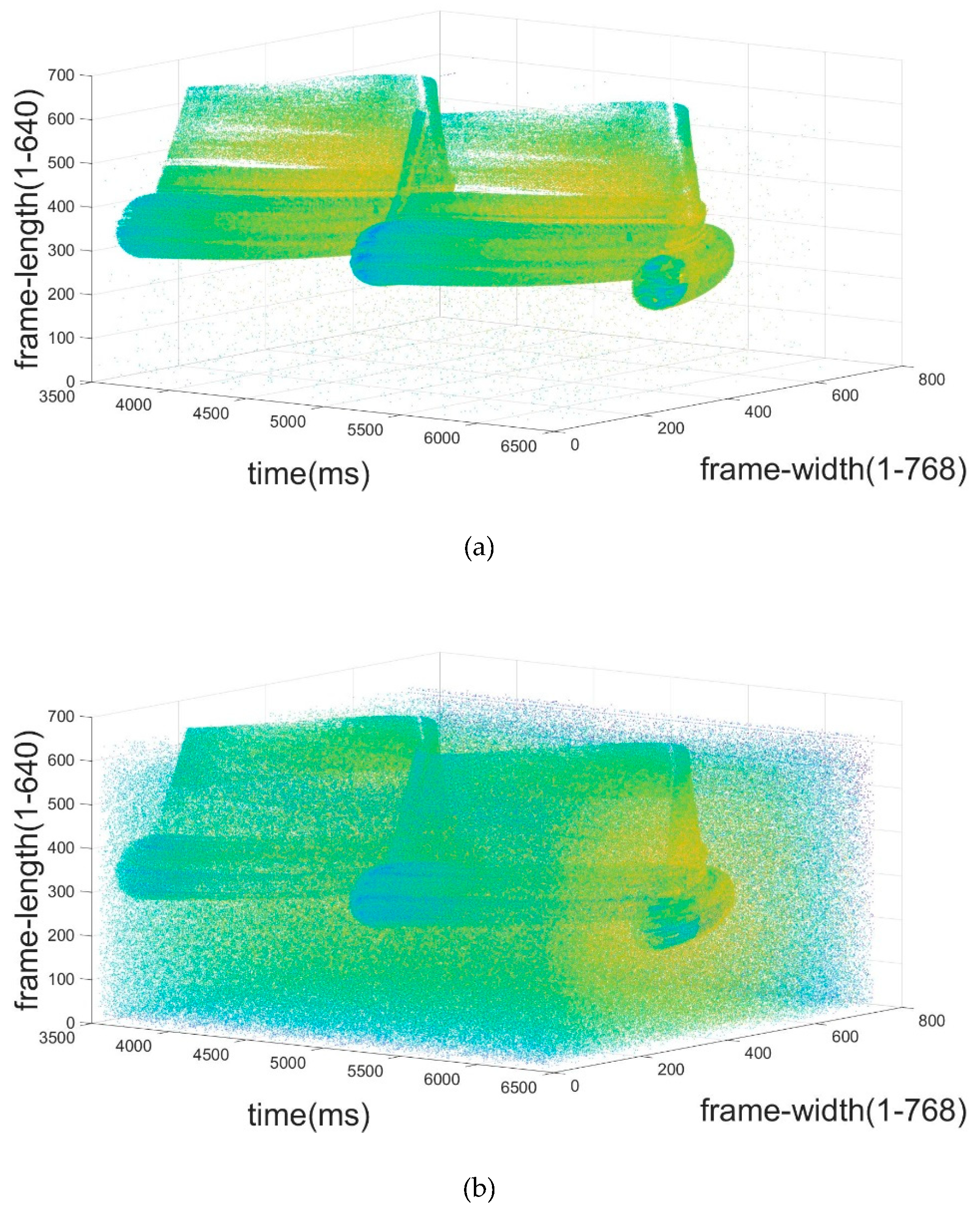
The spatiotemporal image of the original event stream is shown in the Figure 3. It can be seen from the figure that the BA wraps the real event in it, and the average BA frequency is calculated by sampling multiple spatiotemporal positions in the original event stream. There is no real event in the spatiotemporal positions mentioned above, only noise, which is called a noise block. The sampling position and frequency statistics are shown in the Figure 4. The dotted line in the frequency diagram is the average value, which is 0.52 Hz.

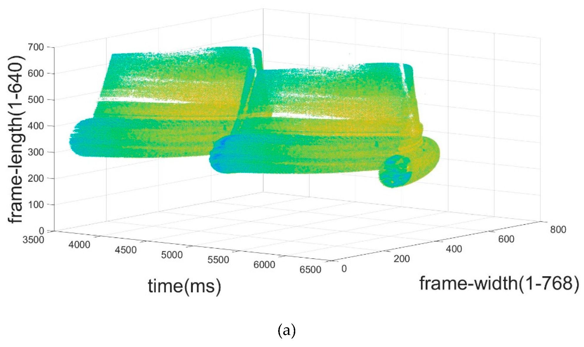
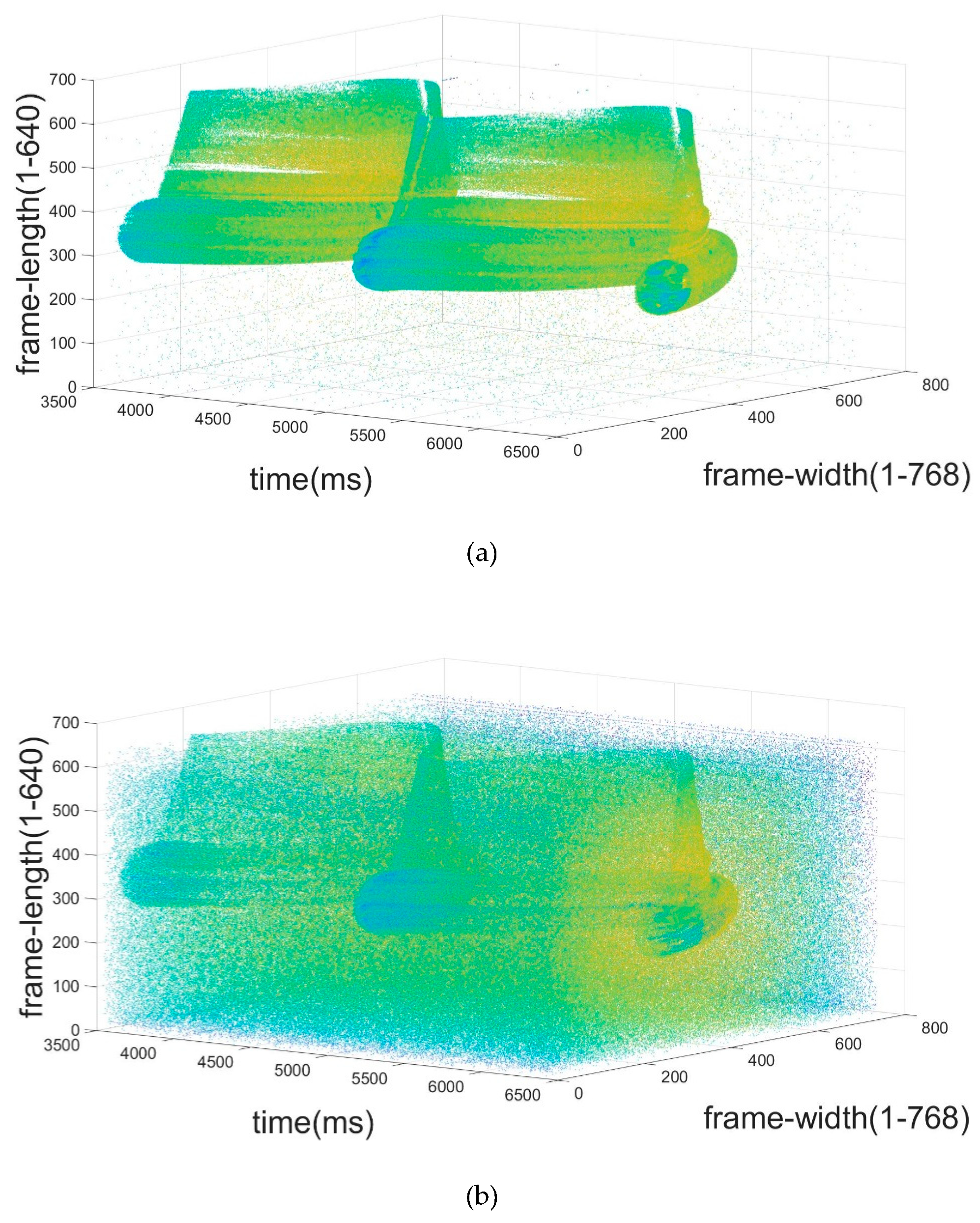
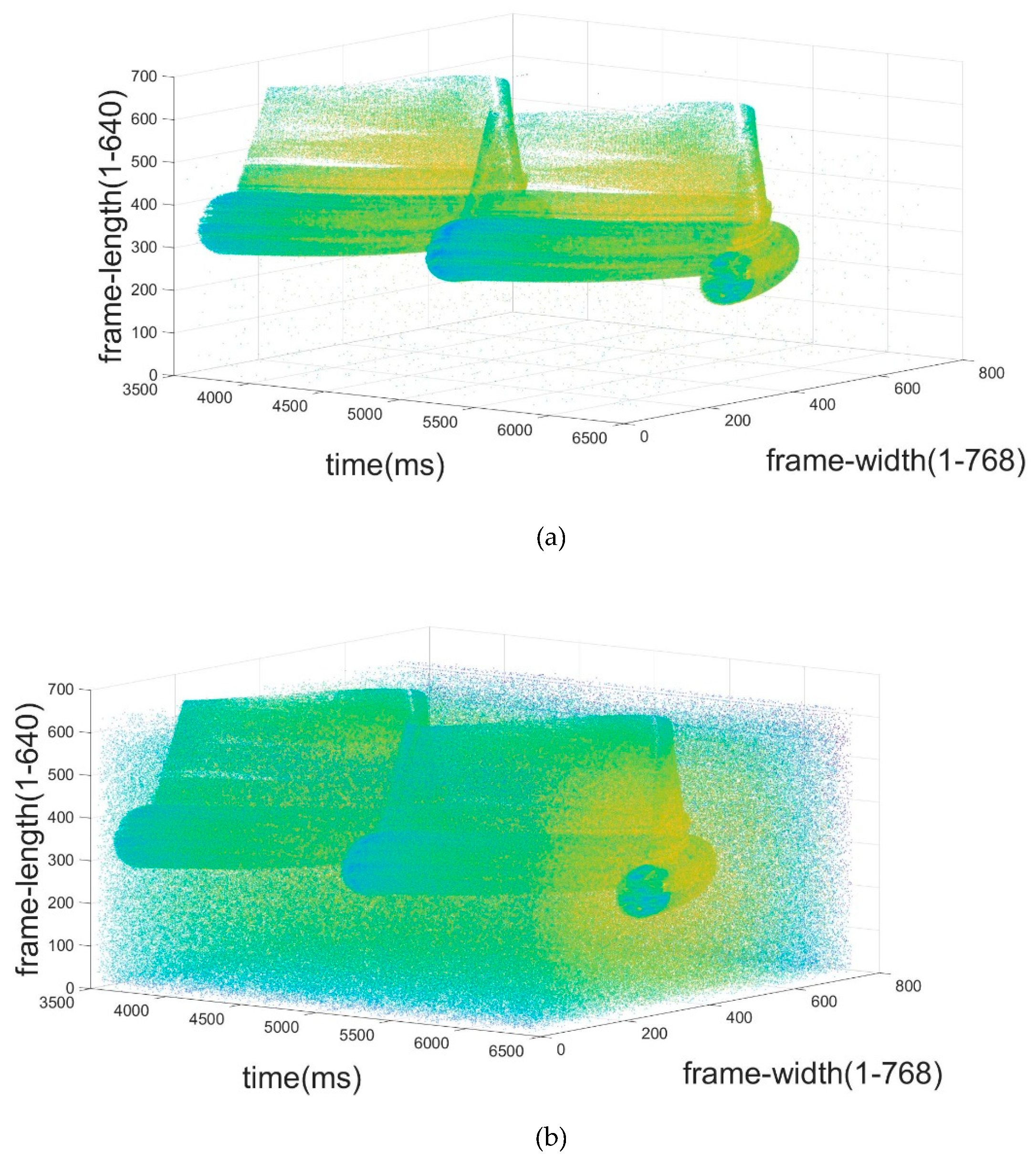
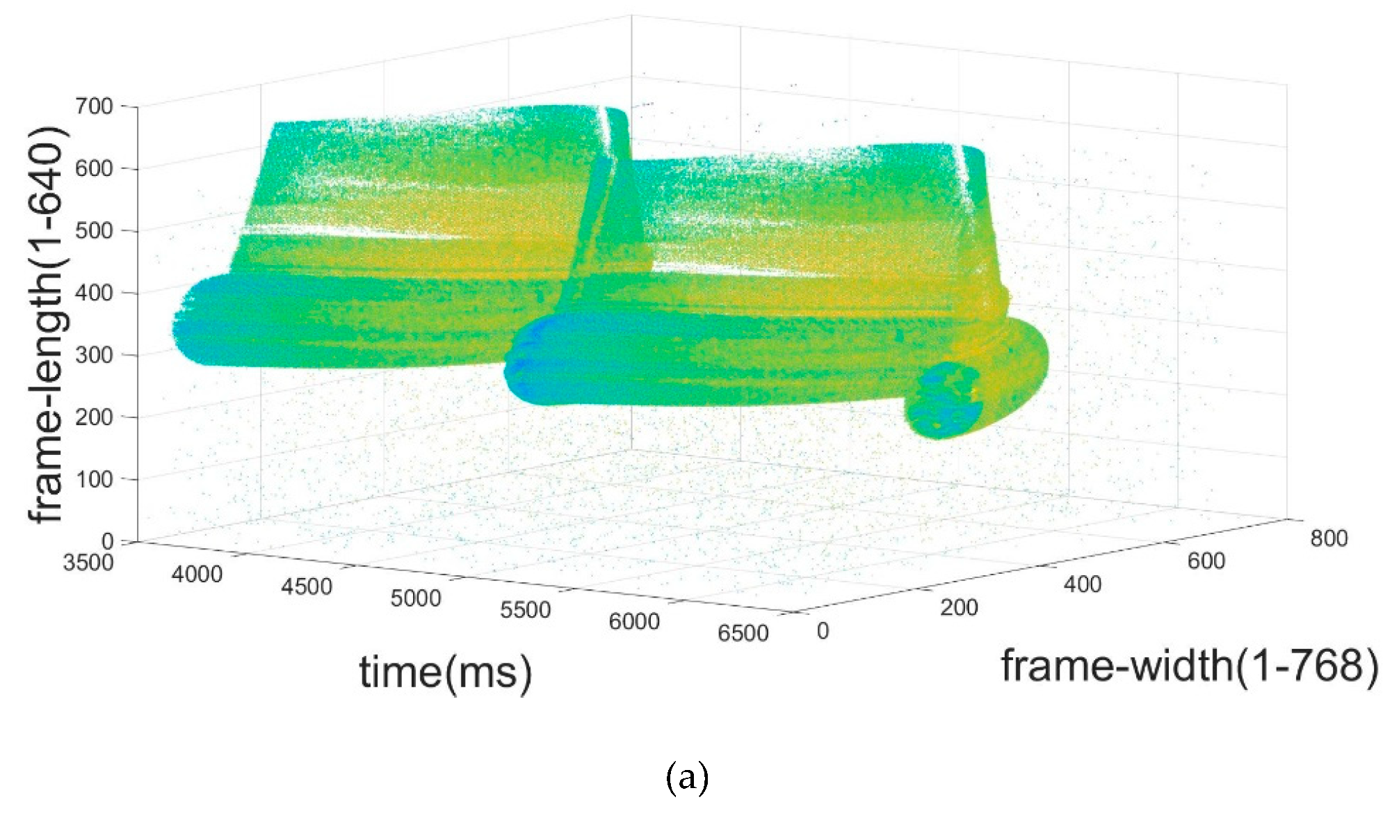
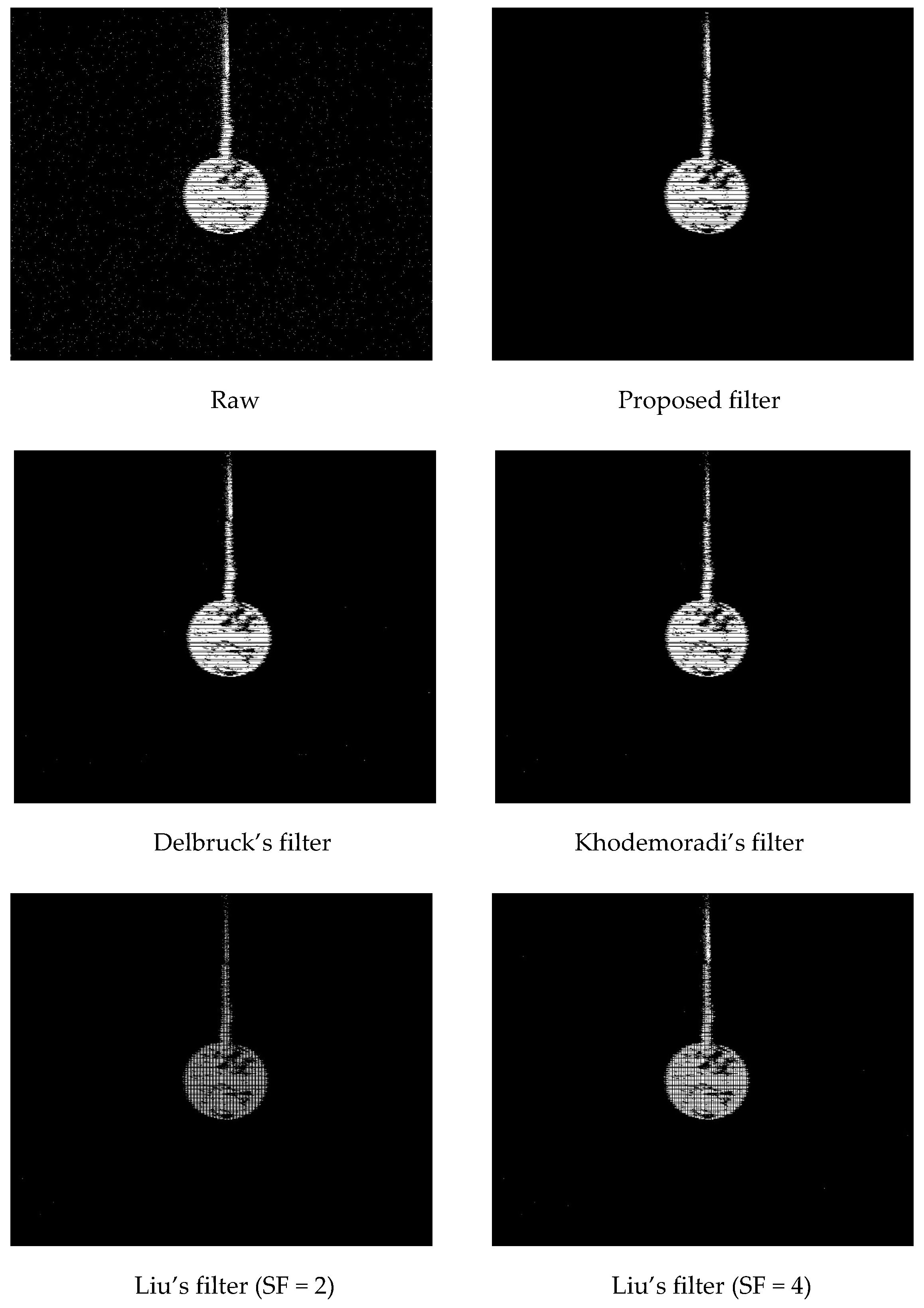
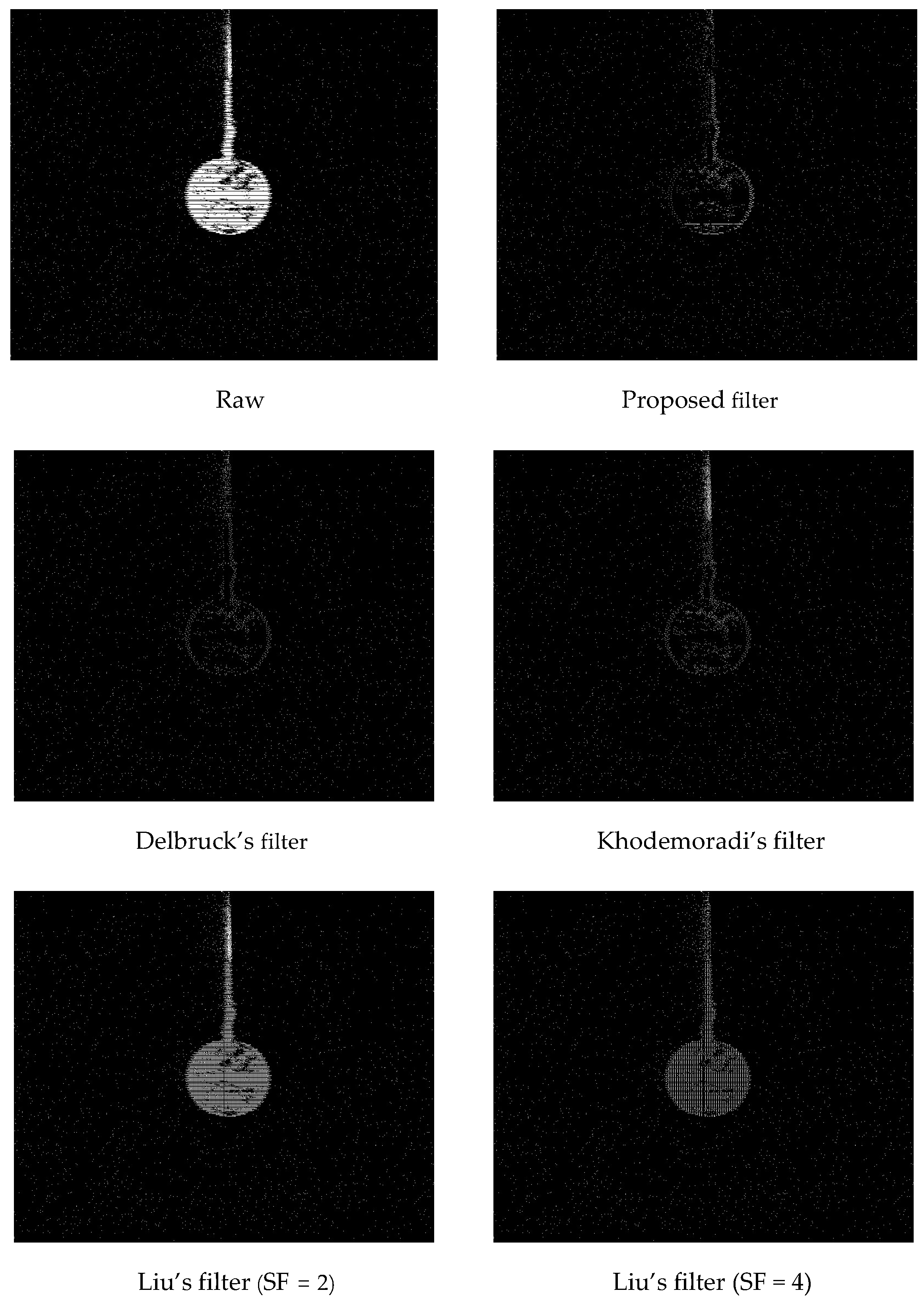
The filtering results are shown in the Figure 5, Figure 6, Figure 7, Figure 8 and Figure 9, where (a) of each graph is the result of denoising and (b) is the filtered noise. It can be seen from the figures that several methods can filter most of the noise, but in the space-time below the pendulum, the result of the comparison method still has some noise in it. This is because the space-time distance between BA is too small, so it was passed. However, the filter is too strict, the real events will be filtered out incorrectly, and the traces of the pendulum ball in the filtered noise will be clearer. The clearest is the result of the subsample factor of 2 in Liu’s filter. The factor is smaller, and the real events of the target are stored in more cells. They cannot support each other, so they are filtered out.

Statistics for the entire event stream. The event stream is divided into 288 segments with a time interval of 10 ms and start time is 3553 ms. The images in Figure 10 are two-dimensional binary images of the original event stream and five results displayed at 3923 ms, and two-dimensional binary images of the filtered noise at that moment. The binary image is obtained by projecting events in the time period of 10 ms into elements at corresponding positions of a matrix of the same size as the focal plane. It can be seen from Figure 11 that the method proposed in this paper has no noise in the area outside the target projection and is denser than the denoising result of Liu’s filter. In the binary image of noise, the outline of the target is clearer than with Delbruck’s filter, which shows that this method filters more real events than Delbruck’s filter, but compared with the other two filters, the real events are better retained.

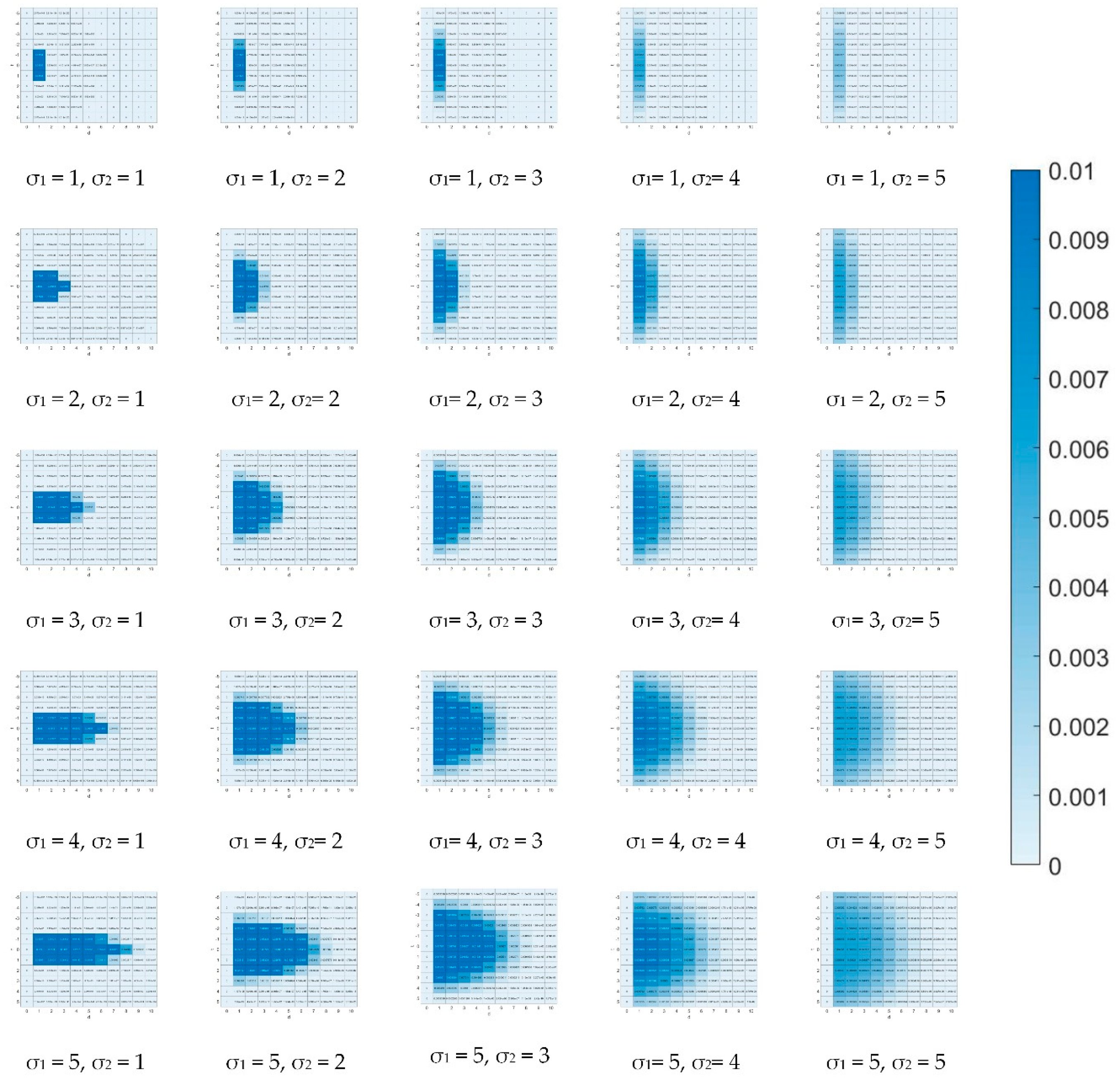
The σ₁ and σ₂ parameters in the evaluation model are set according to the chip resolution and time interval size. If they are set too small, the real event probability of real events will also approach 0. If they are set too large, then the real events probability of events at the edge of space-time will be lower than the events in the center of space-time. The subfigures in Figure 12 are heat maps of evaluation models with different σ₁ and σ₂. The abscissa is the value of d and the ordinate is the value of t. The color corresponds to the weight of the evaluation model. The dark color indicates a larger value, and the light color indicates a smaller value. The heat map shows the change trend of the weight of the evaluation model in time and space by color. As can be seen from Figure 12, when σ₁ and σ₂ are both 2, the events at the edge of time and space will not be affected. As a result, the evaluation model parameters are determined accordingly.

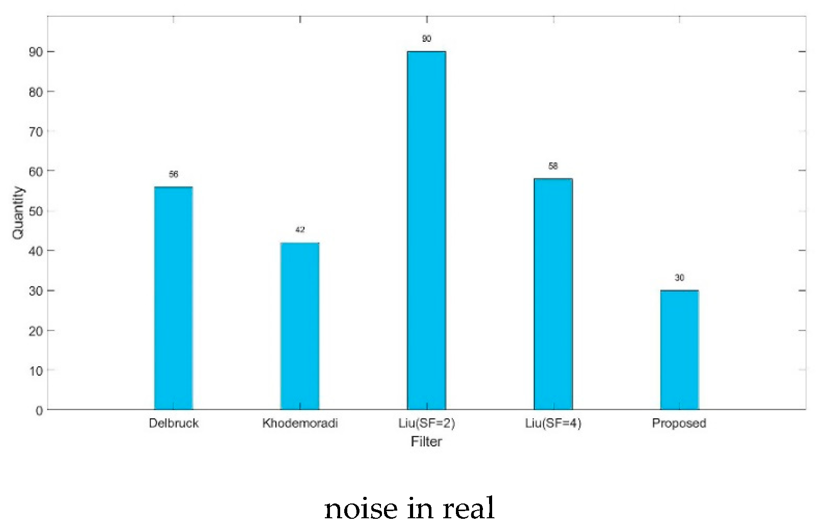
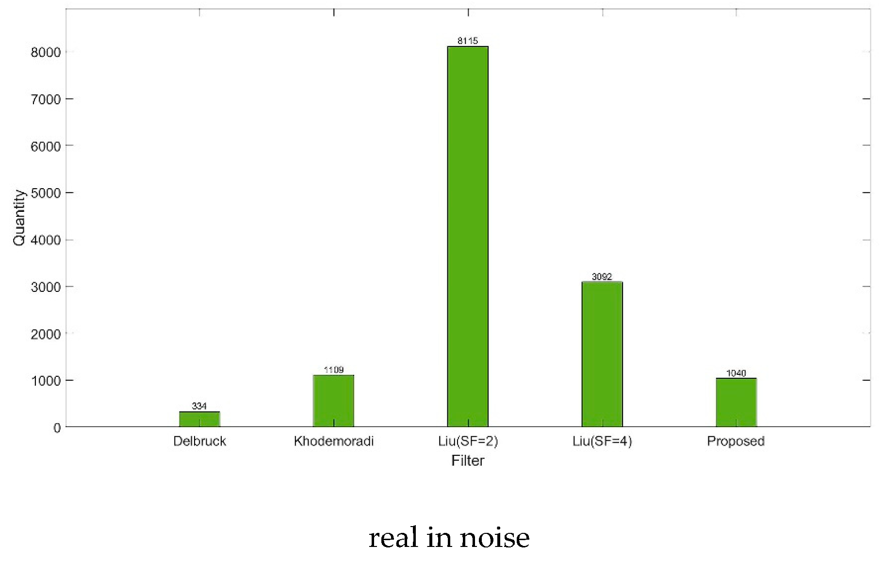
Calculate NIR of results and RIN of the filtered noise at 3923 ms of each filter respectively, as shown in Figure 13. Both σ₁ and σ₂ are 2, they are used in the Gaussian kernel, and the average real event probability of the noise at this moment is 0.0007768.

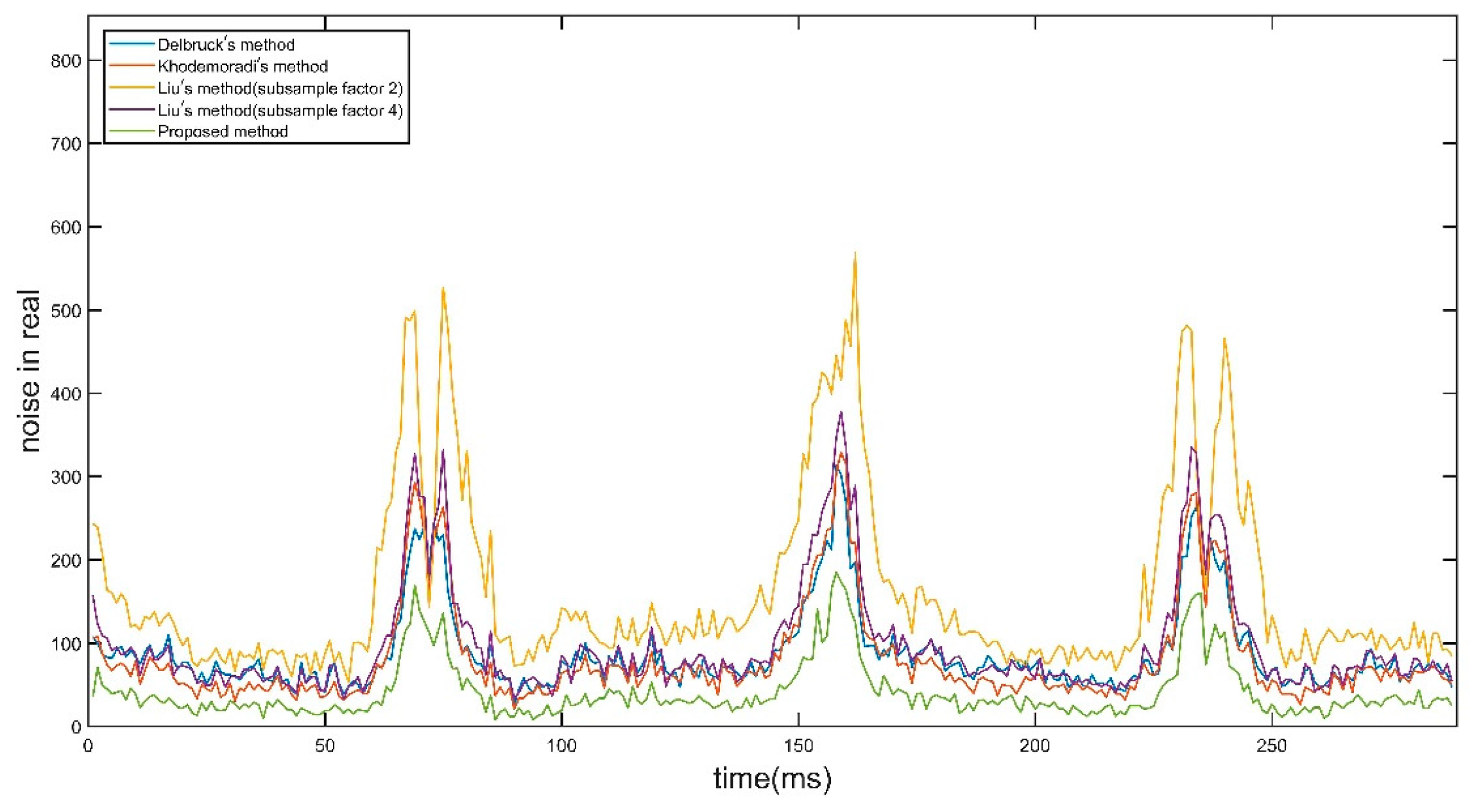
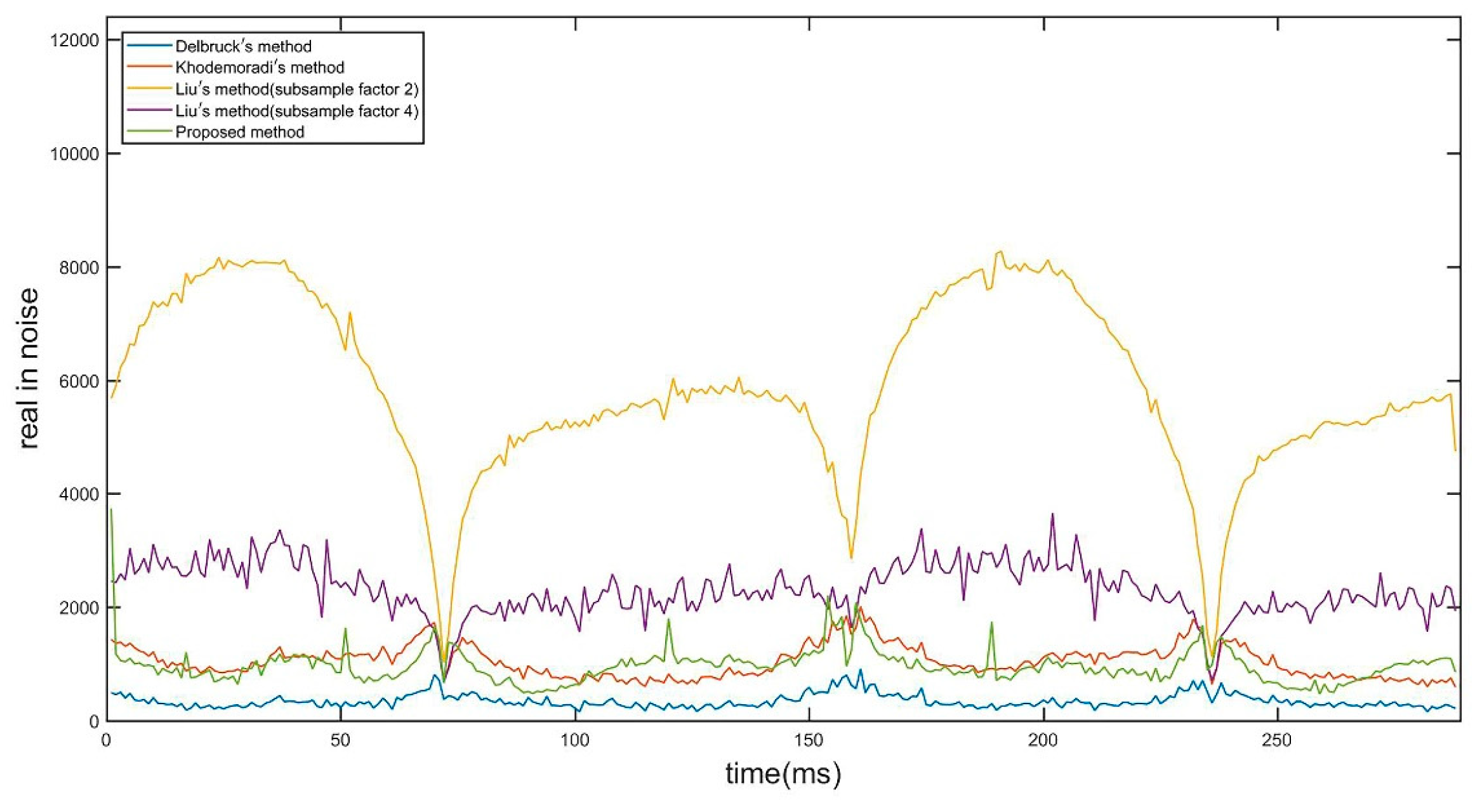
The average real event probability of noise over 288 time periods is 0.001. The Figure 14 and Figure 15 show the comparison of noise in real and real in noise of each filter. It can be seen that the method in this paper is the best of the four methods from the figure of noise in real. This is because the noise determination in this method is based on the density of events, using multiple events to support the identified event to get more accurate results. From the comparison chart of real in noise, it is seen that the value of Delbruck’s filter is the lowest. The method of this article and Khodemoradi’s filter’s indicators are intertwined. Due to insufficient support events for the latest event judgment in the method described in this article, real events are filtered out, and Khodemoradi’s filter caused similar results because it failed to store enough events to support the judgment. The periodic fluctuations in the two figures are due to the periodic movement of the target, the amount of data generated in different time periods is different. The peak in noise in real and the valley in real in noise correspond to the moment when the ball is at the highest point and the speed is the lowest. There are few real events at this moment and more noise, so periodic peaks and valleys appear.

6. Discussion

In this section, the results of these experiments are discussed. It can be seen from the experiments that the method in this paper has good denoising performance, especially the NIR in the denoising results is the lowest among several methods, and the RIN in noise is also ranked second. The advantage of this method on NIR is that the determination of noise is no longer supported by a single event. The spatiotemporal correlation theory determines whether an event is noise or not depending only on whether the eight pixels around the event have an event within a specified time. However, such a standard will cause noise to support the noise and pass when the frequency of noise occurrence is high. In the method of this paper, the determination of noise is based on the density of events in space and time. The determination of noise requires multiple events in a larger range, so the number of incorrect noise passes is reduced.

However, such a judgment method also increases the RIN in the filtered events. Because the projection of the target in the focal plane moves to a new position, and the event density of the pixels at that position does not reach the threshold, the real event will be filtered out by mistake, so the outline of the pendulum can be seen in the experimental noise binary image. The RIN of Delbruck’s filter is optimal also because the events that pass through need only a neighborhood event support, which can protect the target contour events when the target is moving.

It can be seen from the experimental results that the denoising method in this paper can well remove the noise generated during the DVS imaging process. To judge whether an event is noise, only the generated event is required, and more real events are retained. It plays a good supporting role in DVS used in autonomous driving, indoor monitoring, SLAM and other scenarios; it reduces the amount of transmitted data and makes it easier for back-end algorithms to extract target information. In the future, the algorithm’s operation consumption and memory usage will be further optimized.

7. Conclusions

In this paper, we propose a method for denoising the DVS output event stream based on event density and a method for evaluating filter performance without the need for a fixed pattern generator. It can be concluded that this method is more effective than other methods in filtering BA in the event stream. The average noise amount in the denoising result based on event density is less than half of the result of other methods, and the number of filtered real events is also relatively lower. This method reduces the bandwidth required for DVS data transmission, reduces the computational cost of target extraction, and provides the possibility for the application of DVS in more fields.

References

- Delbrück, T.; Linares-Barranco, B.; Culurciello, E.; Posch, C. Activity-Driven, Event-Based Vision Sensors. In Proceedings of the 2010 IEEE International Symposium on Circuits and Systems, Paris, France, 30 May–2 June 2010; pp. 2426–2429. [Google Scholar]
- Lichtsteiner, P.; Posch, C.; Delbruck, T. A 128 × 128 120db 15us latency asynchronous temporal contrast vision sensor. IEEE J. Solid-State Circuits 2008, 43, 566–576. [Google Scholar] [CrossRef] [Green Version]
- Guo, M.; Huang, J.; Chen, S. Live demonstration: A 768 × 640 pixels 200meps dynamic vision sensor. In Proceedings of the 2017 IEEE International Symposium on Circuits and Systems (ISCAS), Baltimore, MD, USA, 28–31 May 207; p. 1.
- Czech, D.; Orchard, G. Evaluating noise filtering for event-based asynchronous change detection image sensors. In Proceedings of the 2016 6th IEEE International Conference on Biomedical Robotics and Biomechatronics (BioRob), Singapore, 26–29 June 2016. [Google Scholar]
- Gallego, G.; Delbruck, T.; Orchard, G.; Bartolozzi, C.; Taba, B.; Censi, A.; Leutenegger, S.; Davison, A.; Conradt, J.; Daniilidis, K. Event-Based Vision: A Survey. arXiv 2019, arXiv:1904.08405. [Google Scholar]
- Weikersdorfer, D.; Adrian, D.B.; Cremers, D.; Conradt, J. Event-based 3d slam with a depth-augmented dynamic vision sensor. In Proceedings of the 2014 IEEE International Conference on Robotics and Automation, Hong Kong, China, 31 May–7 June 2014; pp. 359–364. [Google Scholar]
- Ahn, E.Y.; Lee, J.H.; Mullen, T.; Yen, J. Dynamic vision sensor camera based bare hand gesture recognition. In Proceedings of the 2011 IEEE Symposium On Computational Intelligence For Multimedia, Signal And Vision Processing, Paris, France, 11–15 April 2011; pp. 52–59. [Google Scholar]
- Lee, K.; Ryu, H.; Park, S.; Lee, J.H.; Park, P.; Shin, C.; Woo, J.; Kim, T.; Kang, B. Four dof gesture recognition with an event-based image sensor. In Proceedings of the 1st IEEE Global Conference on Consumer Electronics 2012, Tokyo, Japan, 2–5 October 2012; pp. 293–294. [Google Scholar]
- Joubert, D.; Hébert, M.; Konik, H.; Lavergne, C. Characterization setup for event-based imagers applied to modulated light signal detection. Appl. Opt. 2019, 58, 1305–1317. [Google Scholar] [CrossRef]
- Alzugaray, I.; Chli, M. Asynchronous corner detection and tracking for event cameras in real time. IEEE Robot. Autom. Lett. 2018, 3, 3177–3184. [Google Scholar] [CrossRef] [Green Version]
- Mueggler, E.; Huber, B.; Scaramuzza, D. Event-based, 6-dof pose tracking for high-speed maneuvers. In Proceedings of the 2014 IEEE/RSJ International Conference on Intelligent Robots and Systems, Chicago, IL, USA, 14–18 September 2014; pp. 2761–2768. [Google Scholar]
- Miguel, R.A.; Susana, O.-C.; Jorge, R.; Federico, S.-I. American sign language alphabet recognition using a neuromorphic sensor and an artificial neural network. Sensors 2017, 17, 2176. [Google Scholar]
- Barrios-Avilés, J.; Rosado, A.; Medus, L.; Bataller-Mompeán, M.; Guerrero Martinez, J. Less data same information for event-based sensors: A bioinspired filtering and data reduction algorithm. Sensors 2018, 18, 4122. [Google Scholar] [CrossRef] [PubMed] [Green Version]
- Celepixel Technology Co. Ltd. Available online: http://www.celepixel.com (accessed on 5 March 2020).
- Samsung Smartthings Vision. Available online: https://www.samsung.com/au/smart-home/smartthings-vision-u999/ (accessed on 5 March 2020).
- Nozaki, Y.; Delbruck, T. Temperature and parasitic photocurrent effects in dynamic vision sensors. IEEE Trans. Electron Devices 2017, 64, 3239–3245. [Google Scholar] [CrossRef] [Green Version]
- Jing, H.; Guo, M.; Chen, S. A dynamic vision sensor with direct logarithmic output and full-frame picture-on-demand. In Proceedings of the 2017 IEEE International Symposium on Circuits and Systems (ISCAS), Baltimore, MD, USA, 28–31 May 2017. [Google Scholar]
- Liu, H.; Brandli, C.; Li, C.; Liu, S.; Delbruck, T. Design of a spatiotemporal correlation filter for event-based sensors. In Proceedings of the 2015 IEEE International Symposium on Circuits and Systems (ISCAS), Lisbon, Portugal, 24–27 May 2015; pp. 722–725. [Google Scholar]
- Benosman, R.; Clercq, C.; Lagorce, X.; Ieng, S.; Bartolozzi, C. Event-based visual flow. IEEE Trans. Neural Netw. Learn. Syst. 2014, 25, 407–417. [Google Scholar] [CrossRef] [PubMed]
- Brändli, C.P. Event-Based Machine Vision. Ph.D. Thesis, ETH Zurich, Zürich, Switzerland, 2015. [Google Scholar]
- Khodamoradi, A.; Kastner, R. O(n)-space spatiotemporal filter for reducing noise in neuromorphic vision sensors. IEEE Trans. Emerg. Top. Comput. 2018. [Google Scholar] [CrossRef]
- Delbrück, T. Frame-free dynamic digital vision. In Proceedings of the International Symposium on Secure-Life Electronics, Advanced Electronics for Quality Life and Society, Tokyo, Japan, 6–7 March 2008; p. 26. [Google Scholar]
Figure 1.
This is the data of a moving car. The sensor size is 768 × 640. There are real events and a lot of noise in the data. The color indicates the gray information of the event.
Figure 2.
Schematic of the spatiotemporal neighborhood. The red-point indicates a newly arrived event at t1, the surrounding yellow part indicates the spatial neighborhood of the new-arrival event, and delta, t, which is the time period before t1 is the time neighborhood of the event. The time neighborhood and spatial neighborhood form a spatiotemporal neighborhood.