Planetary-Gearbox Fault Classification by Convolutional Neural Network and Recurrence Plot


1
Faculty of Mechanical and Electrical Engineering, Kunming University of Science and Technology, Kunming 650500, China
2
Faculty of Mechanical Engineering, Department of Automation, Lublin University of Technology, 20-618 Lublin, Poland
*
Author to whom correspondence should be addressed.
Appl. Sci. 2020, 10(3), 932; https://doi.org/10.3390/app10030932
Submission received: 19 December 2019
/
Revised: 21 January 2020
/
Accepted: 21 January 2020
/
Published: 31 January 2020
(This article belongs to the Special Issue Selected Papers from IMETI 2018)
Abstract
:Recurrence-plot (RP) analysis is a graphical tool to visualize and analyze the recurrence of nonlinear dynamic systems. By combining the advantages of the RP and a convolutional neural network (CNN), a fault-classification scheme for planetary gear sets is proposed in this paper. In the proposed approach, a vibration is first picked up from the planetary-gear test rig and converted into an angular-domain quasistationary signal through computed order tracking to eliminate the frequency blur caused by speed fluctuations. Then, the signal in the angular domain is divided into several segments, and each segment is processed by the RP to constitute the training sample. Moreover, a two-dimensional CNN model was developed to adaptively extract faulty features. Experiments on a planetary-gear test rig with four conditions under three operating speeds were carried out. The results of measured vibration demonstrated the validity of CNN and recurrence plot analysis for the fault classification of planetary-gear sets.
1. Introduction
Due to their power capability in a compact, lightweight form and variable transmission ratio, planetary-gear trains are key units of rotating machinery that are widely used in helicopters, wind turbines, and other mechanical transmission systems. However, harsh operating conditions make components in planetary gearboxes, such as gears and bearings, prone to failure. Therefore, it is urgent to develop effective diagnostic approaches to detect the operating conditions of a mechanical transmission system.
Compared with conventional fixed-axis gear sets, the structures of planetary gearboxes are more complicated and generally composed of a planet carrier, a sun gear, a ring gear, and several planets. Planet gears not only spin around their own shaft, but also revolve around the center of the sun gear. Thus, the perceived vibration from the planetary gear set characterizes heavy amplitude, frequency, and phase demodulation caused by gears or bearing faults, gear meshing motion, and time-varying transfer paths.
Currently, popular approaches for extracting fault features caused by planetary gear sets are vibration-based methods, which include the vibration-separation technique [1], amplitude and frequency demodulation [2,3]. However, these conventional signal-processing approaches have some disadvantages. First, when we use these approaches, the operational characteristics and failure mechanisms of planetary-gear trains should be considered. Second, it is difficult to recognize fault features form various faults.
On the other hand, AI techniques have recently been used in the field of condition monitoring and fault diagnosis. AI techniques could be employed in the condition monitoring and fault diagnosis of rotating machinery by taking expert knowledge into consideration. In fact, some convolutional-neural-network (CNN) studies reported on the fault identification of complex machinery transmission systems. For example, the spectrum of bearing housing vibration is processed by fast Fourier transform to identify faults with the CNN [4]. The time- and frequency-domain indicators were combined with the CNN for fault classification of a fixed shaft gearbox in [5,6].
The main deep-learning schemes generally have the advantage of taking 2D images as inputs. The perceived vibration is converted into time-frequency [7] or time-scale images by continuous wavelet transform (CWT), short-time Fourier transform (STFT), and Fourier transform (FT), which aim to be combined with the CNN for intelligent fault diagnosis [8]. Recurrence-plot (RP) analysis [9] is a powerful tool to locate nonstationary structural changes and transitions occurring in the dynamic system. It can be employed to study the response of a planetary-gear set and visualize the recurrence behavior of a faulty system [10,11]. RP results are 2D images that make the RP and CNN combination convenient. In this paper, a combination scheme of a CNN and angular-domain recurrence-plot analysis is proposed. The validity of the proposed scheme is experimentally demonstrated on a planetary-gear test rig.
This paper is arranged as follows. Angular-domain recurrence-plot analysis is introduced in Section 2. Subsequently, the CNN principle is briefly described in Section 3. The proposed approach is discussed in Section 4. The experiment on the planetary-gear test rig and the corresponding analysis results are presented in Section 5. Finally, conclusions are drawn in Section 6.
2. Materials and Methods
2.1. Angular-Domain Recurrence-Plot Analysis
Because the recurrence plots of the raw vibration can be distorted by speed fluctuations, it is conceivable to remove the distortions before carrying out the RP to improve the accuracy of fault classification. Therefore, the well-known equiangle resampling scheme in computer order tracking (COT) was employed to convert the observed time series into an angular-domain quasistationary one that can avoid the frequency blur caused by speed fluctuations. More details can be found in [12,13].
2.1.1. Phase-Space Reconstruction in Angular Domain
The possible states of the dynamic system can be represented by phase-space reconstruction that reconstructs the one-dimensional time series into a high-dimensional phase space to unfold the attractor and reflect characteristics of a dynamic system. The main methods of phase-space reconstruction were proposed, and the time-delay method was employed in this paper. In the same way, for resampled angular-domain observations, angle-delay vector in d-dimensional space could be reconstructed as in [14] by:
where is the angle delay and d represents the embedding dimension. It is easy to see from Equation (1) that either determining angle delay or calculating embedding dimension d is critical to obtain a better reconstruction result.
2.1.2. Determination of Embedding Dimension
To determine a suitable embedding dimension in phase-space reconstruction, some methods were proposed, such as computing some invariant on the attractor, singular-value decomposition, and false nearest neighbors (FNN) [15]. In this paper, the FNN method was used to analyze angular-domain data series, which is similar to the discrete-time series in theory. In d-dimensional phase space, the square of Euclidean distance between point and rth nearest neighbor of , can be presented as in [14] by:
From the dth to ()th dimension, corresponding Euclidean distance is changed into
In engineering applications, the observed vibration may have limited length and low signal-to-noise ratio (SNR). In this situation, by only considering the nearest neighbors [14], e.g., , the criterion to identify the false neighbors in the angular domain can be expressed as in [14]:
where is the threshold (without losing generally, it is set to 2). A suitable d is determined with the value of the first minimum of the FNN [9].
2.1.3. Determination of Angle Delay
The angle delay is also a critical parameter in phase-space reconstruction. If is too small, the two trajectories in the phase space are too closed, which makes it impossible to unfold the attractor. If is chosen largely, the co-ordinate components are statistically independent, and even the trajectory projection of chaotic attractors is without correlation.
To obtain a proper , some approaches were proposed, including the average displacement autocorrelation function and mutual information [16] employed in this study. We considered nonlinear system (S,Q), which was composed of angular-domain discrete data series and delay vector . Assume that S was measured. Mutual information could be computed as in [17] by:
where , represent the probability of in S and in Q, respectively. denotes the joint probability of and . A suitable angle delay was selected at the value of the first minimum of the mutual-information function. Details about mutual information can be found in [16,17].
2.2. Briefs on Recurrence Plot
Recurrence-plot analysis measures the recurrence behavior of a trajectory in phase space, which visualizes the structural changes and transitions of a dynamic system by an image. In this research, the angular-domain data series were used as the analysis data of the recurrence-plot analysis, and the mathematical expression of recurrence matrix at resampling angles i and j can be expressed as in [9] by:
where is a threshold distance, is the Heaviside function, N is the number of the angular-domain data series points, and is the Euclidean norm. A discussion on the threshold can be found in [18], and more details about recurrence-plot analysis and setting parameters can be seen in [9,18].
3. Briefs on Convolutional Neural Network
3.1. Typical Configuration of Convolutional Neural Network
A CNN generally contains five layers: the convolutional, activation, pooling, fully connected, and softmax layers. Convolutional layers are composed of several convolutional kernels that abstract and adaptively learn features from the input to obtain feature maps. The first feature map is computed by convolving the input images with the first convolutional kernel, and the next feature map is obtained from the previous output through multiplying the shared weight and adding the bias. Then, the nonlinear activation function is applied on the above-mentioned convolutional results, which is defined by sigmoid or a rectified-linear-unit (ReLU) function [19]. The ReLU is widely applied after the output of every convolutional and fully connected layer.
In the classification stage of the CNN model, there is generally a fully connected layer and classifier that mainly integrate and classify information from the previous layer. A softmax regression classifier is always placed at the last layer to estimate the probability of multiple faults. Cross-entropy is generally used as the loss function to represent the error between the true and estimated value. Weight matrix and bias term are optimized by the adaptive-moment-estimation method (ADAM). ADAM is able to dynamically adjust the learning rate of each parameter through first- (average) and second-order (variance) moment estimation [20]. Thus, it is appropriate for nonstationary objectives and engineering vibration data with a low SNR. Moreover, in applications, this method can efficiently compute and needs little memory, which is suitable for processing long data.
3.2. Evaluation Indicators of CNN Model
To quantify the performance of different methods, four evaluation indicators were employed: accuracy, precision, recall, and -score. The calculation of these indicators is shown in [4]. In engineering applications, the condition-monitoring system ideally triggers an alarm for real faults, and avoids false or missed triggers. Therefore, a good classification method that maximizes all evaluation indicators is required. More details about CNN setting parameters and configurations can be found in [4,5,8].
4. CNN Combined with Angular-Domain RP for Fault Classification of Planetary Gearboxes
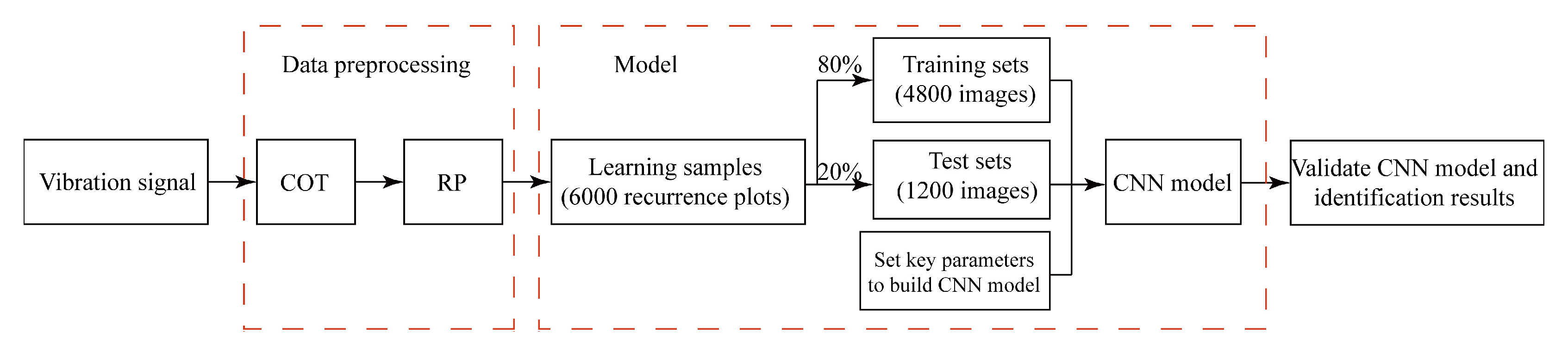
In this study, a combination of a CNN and angular-domain RP for the fault classification of planetary gearboxes is proposed. The corresponding schematic is shown in Figure 1.
The main steps of the proposed scheme are listed as follows:
- Vibration-signal acquisition and processing. Raw vibration of the planetary gearbox is picked up synchronously with the tacho plus trains of the reference shaft. Then, equiangle resampling is performed to convert the data series into those in the angular domain.
- Construction of training dataset. Vibration data series are first divided into segments. For a planetary gearbox with a fixed annulus gear, the transmission ratio of the planet carrier and sun gear can be expressed bywhere , are the tooth numbers of the sun and ring gear, respectively. For the minimal common complete integral period of the sun gear and planet carrier, the sun gear needs to rotate circles, and the carrier rotates circles. Therefore, to ensure each segment covering the meshing vibration of all teeth, the corresponding rotating circles of the sun gear should not be less than .We assumed that the rotating speed of the sun gear was , and the total time of the observed signal was T. To save computation time, the resampled length data in the angular domain can be expressed by:where is resampling points per revolution. Thus, the points of each segment equal to . Then, to a condition with three operating speeds, each segment was randomly selected to constitute the training sample.
- Build CNN model and set parameters. The configuration of a 2D CNN was used. Several key parameters, such as learning rate, the size of convolutional kernels, number of iterations, and nodes of fully connected layers were set and are discussed in the next section.
- Identification results and evaluation of CNN model.
5. Experiments and Discussion
5.1. Planetary-Gearbox Test Rig
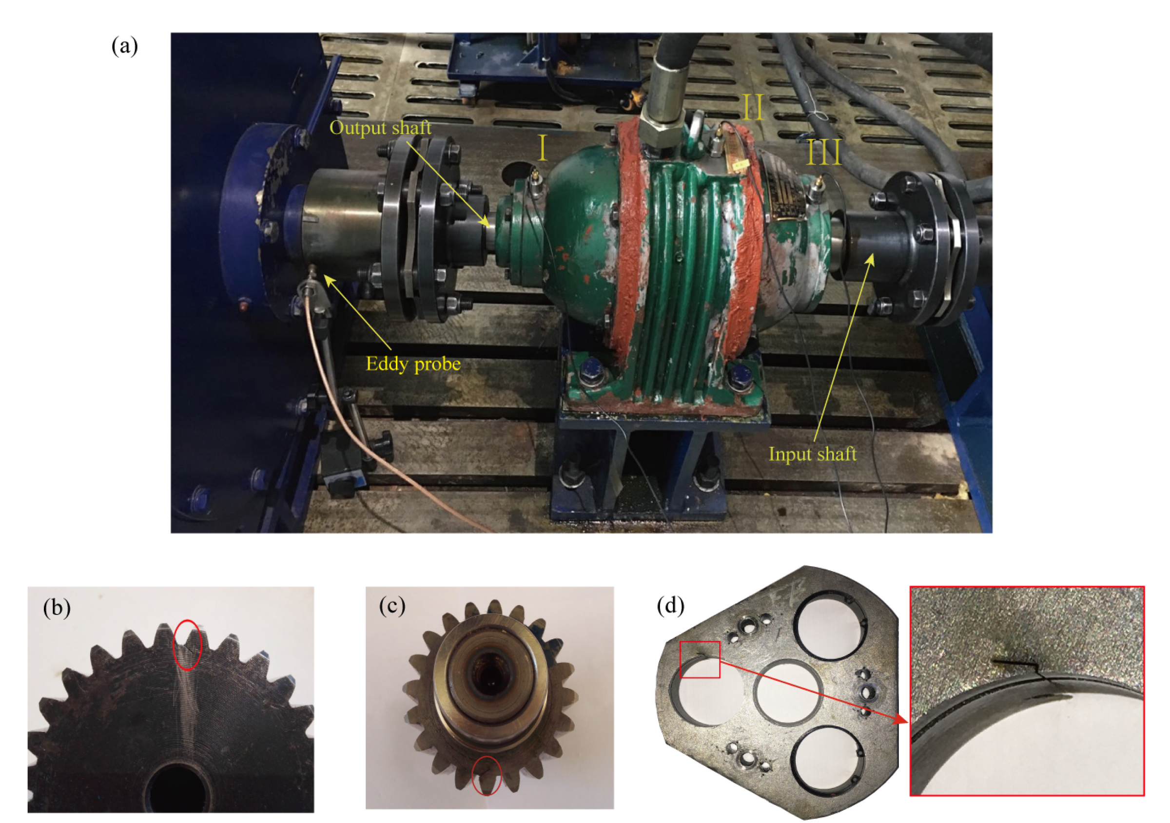
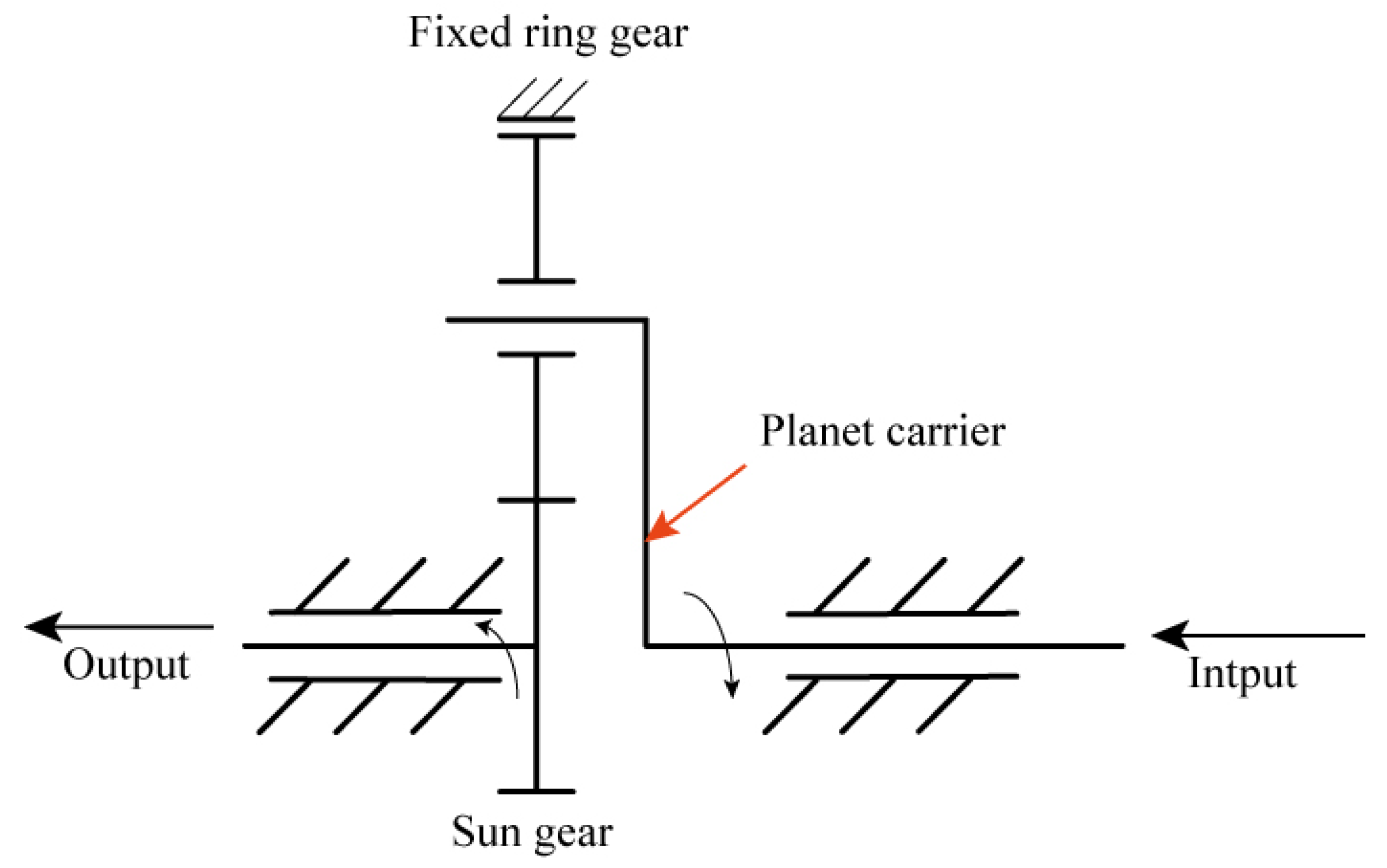
In order to validate the validity of the proposed approach, an experiment with four conditions under three operating speeds was carried out on a planetary-gear test rig (with one 28-tooth sun gear, three 20-tooth planet gears, a 71-tooth fixed ring gear, and a carrier; the gear modulus was 2.25), shown in Figure 2a, where the output shaft was connected with the sun-gear shaft by a coupling, and the planetary carrier was the input. The kinematical schema of the experiment planetary gearbox can be found in Figure 3. An eddy probe was fixed by a magnetic base to measure the tacho impulse trains of the output shaft, and three accelerometers were respectively mounted on the planetary-gearbox housing, as shown in Figure 2a. The data were implemented by an NI USB 9234 card with a sampling rate of 51.2 kHz.
In this study, a vibration picked up by accelerometer II close to the ring gear was used. Four conditions of the planetary gearbox, that is, normal; planet gear-root crack; sun gear with a tooth-root crack; and planet carrier with a crack, are shown in Figure 2b–d. The tooth-root-crack length of the faulty planet and sun gear was 4 and mm, respectively. The crack size of the carrier was 21 mm length, 5 mm depth, and mm width.
5.2. Data Preprocessing and Model Design
5.2.1. Data Preprocessing
First, taking the sun gear as the reference shaft, a raw vibration with 600 s was converted into those in the angular domain by the COT, which eliminates speed fluctuations. Sampling points per revolution in the angular domain were selected to be 1024.
Subsequently, the data series in the angular domain were divided into several segments. According to Equation (7), data length corresponds to 99 circles of the sun gear. Then, each segment was divided in this way. To reduce computation time, 200 resampling points were selected in a revolution of the sun gear. Thus, the number points of the resampled data series were , and each segment was points in the condition that the rotating speed of the sun gear is 800 r/min. In the time domain, we could calculate the time of a complete circle under different rotating speeds. For example, when the rotating speeds of the output shaft were 800, 700, and 600 r/min, the lengths of the data series in the time domain were 7.425, 8.486, and 9.9 s, respectively, when resampling ratewas 2000 points per second. Thus, each segment was randomly selected as 7.5, 8.5, and 10 s of the total 600 s of observed vibration.
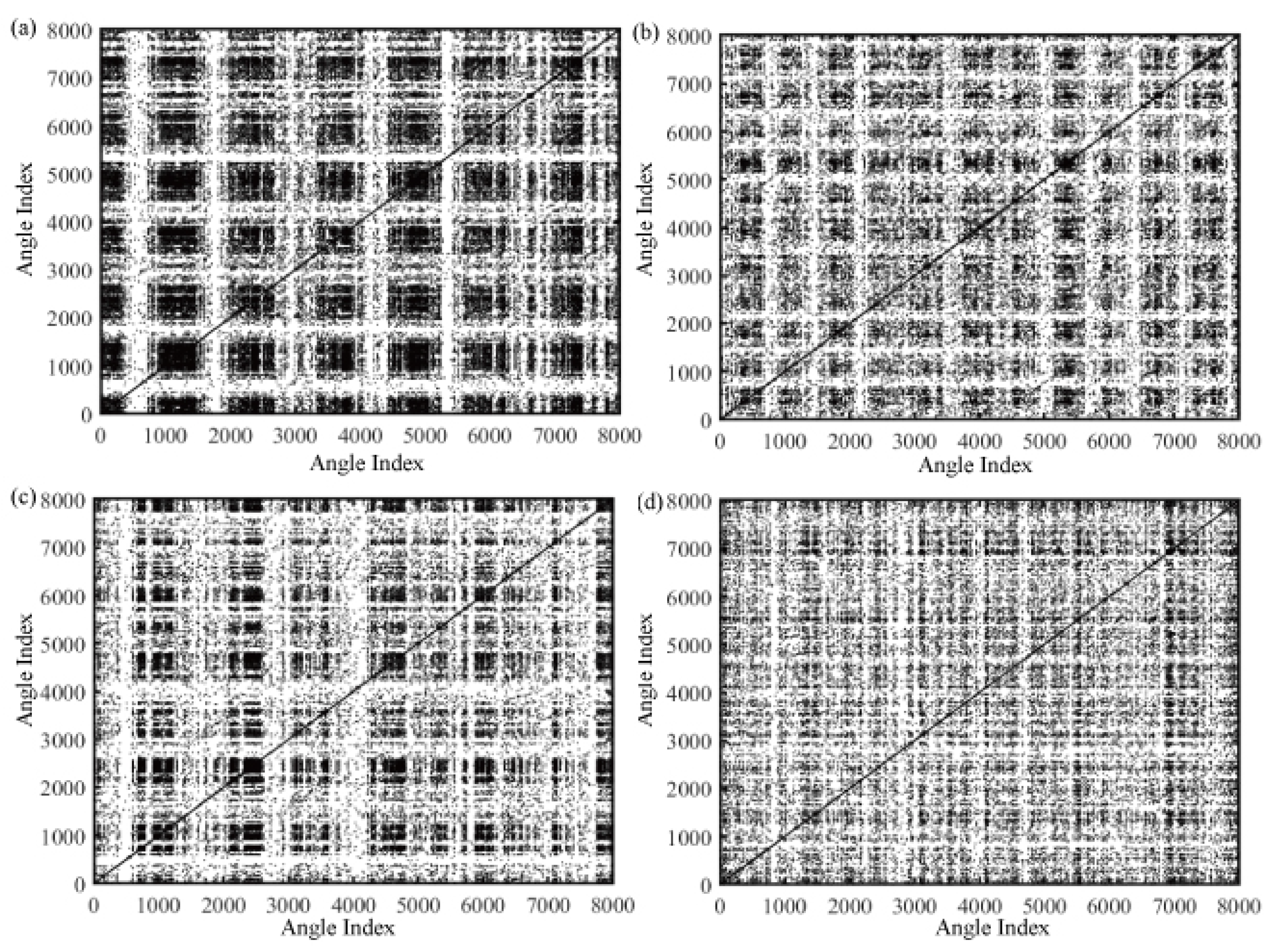
Then, all segments were processed by recurrence-plot analysis to obtain 2D images as the training sample. The recurrence plots in the angular domain of the four conditions with = 800 r/min are presented in Figure 4. In order to show the obtained recurrence-plot differences between multifault categories, only 8000 of 19,760 points are shown. Angle delay and embedding dimension d were determined by the FNN and mutual-information function, respectively. Threshold was determined by the standard deviation of the observed angular-domain signal [11]. The vertical distance between these lines can be seen in Figure 4, signals’ intermittent behavior with a characteristic angle scale [21] of components caused by faults. Small fluctuations could also be seen for all considered conditions, but these differences were slight and not conducive to quantitatively distinguish. Moreover, for the same condition, they may have been slightly different, so it was hard to determine the planetary-gearbox failure type only on the basis of recurrence plots.
5.2.2. Model Design
The configuration of the two-dimensional CNN consisted of two convolutional layers, two pooling layers, three fully connected layers, and a softmax regression. Cross-entropy was employed as the loss function, and several fundamental parameters of the CNN model are listed in Table 1.
5.3. Results and Discussion
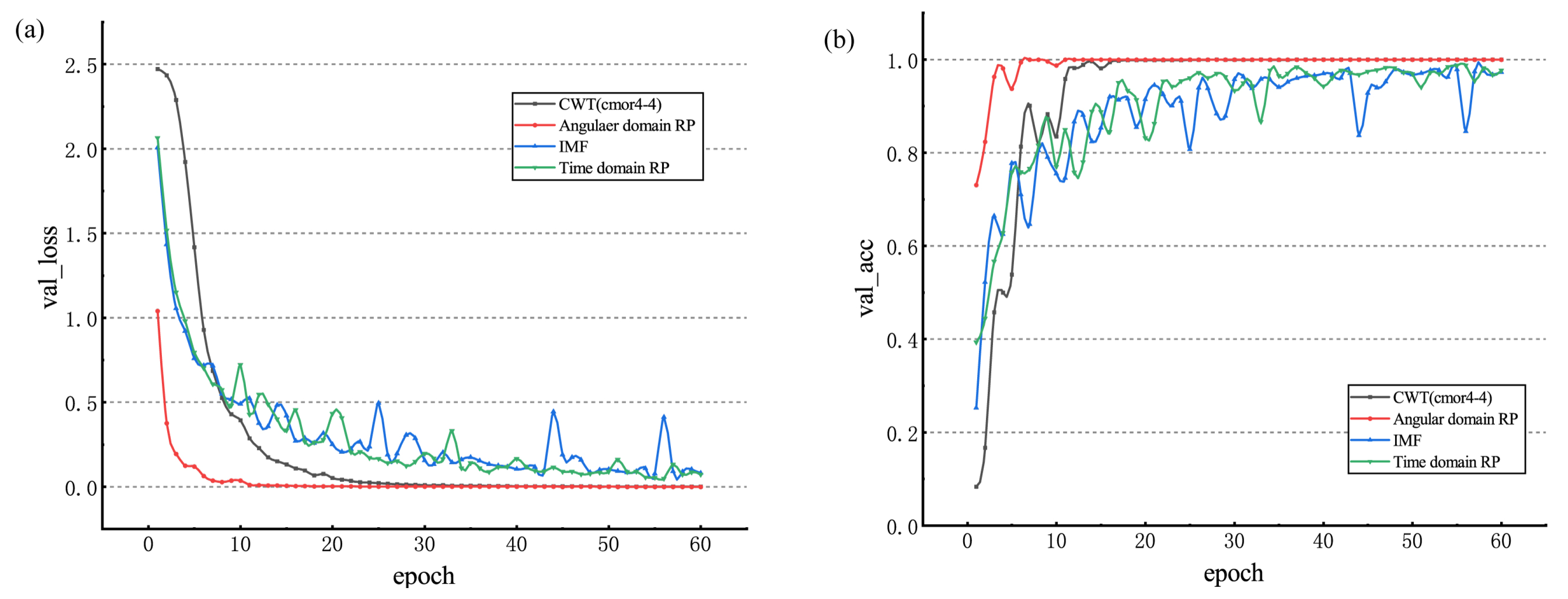
Three comparative methods were utilized in this study. The RP of the time domain, continuous wavelet transform (cmor4-4), and the first six maximal peak values of the intrinsic mode function (IMF) generated by the empirical mode decomposition (EMD) of the experiment data [22] were employed to validate the performance of the proposed method. The comparative results of the four approaches are shown in Figure 5. Figure 5a shows the valuation loss, which was used to measure the extent of prediction error. The closer the prediction probability to 1 was, the closer the loss value to zero was. For the time-domain recurrence-analysis (green line) and EMD (blue line) methods, loss values were significantly higher than those of other methods (loss value stabilizes at 0), with more obvious fluctuations. Figure 5b shows valuation accuracy, which is defined as the ratio of the true number to the total number. The higher the accuracy is, the better the classification of the model. According to Figure 5b, the valuation accuracy of the proposed method (red line) and CWT (black line) was up to 100%. For the same CNN model, the valuation loss and accuracy of the IMF were fluctuant, which explains why this method failed to effectively extract fault features. Comparing the results of recurrence analysis, the proposed method was better than that in time domain due to eliminating the rotational fluctuations. Although both angular-domain recurrence analysis and CWT could obtain effective results, convergence speed was different. The valuation accuracy of the proposed method reached 100% and valuation loss was about 0% with epoch = 15, which demonstrated that convergence speed was better than that of the CWT.
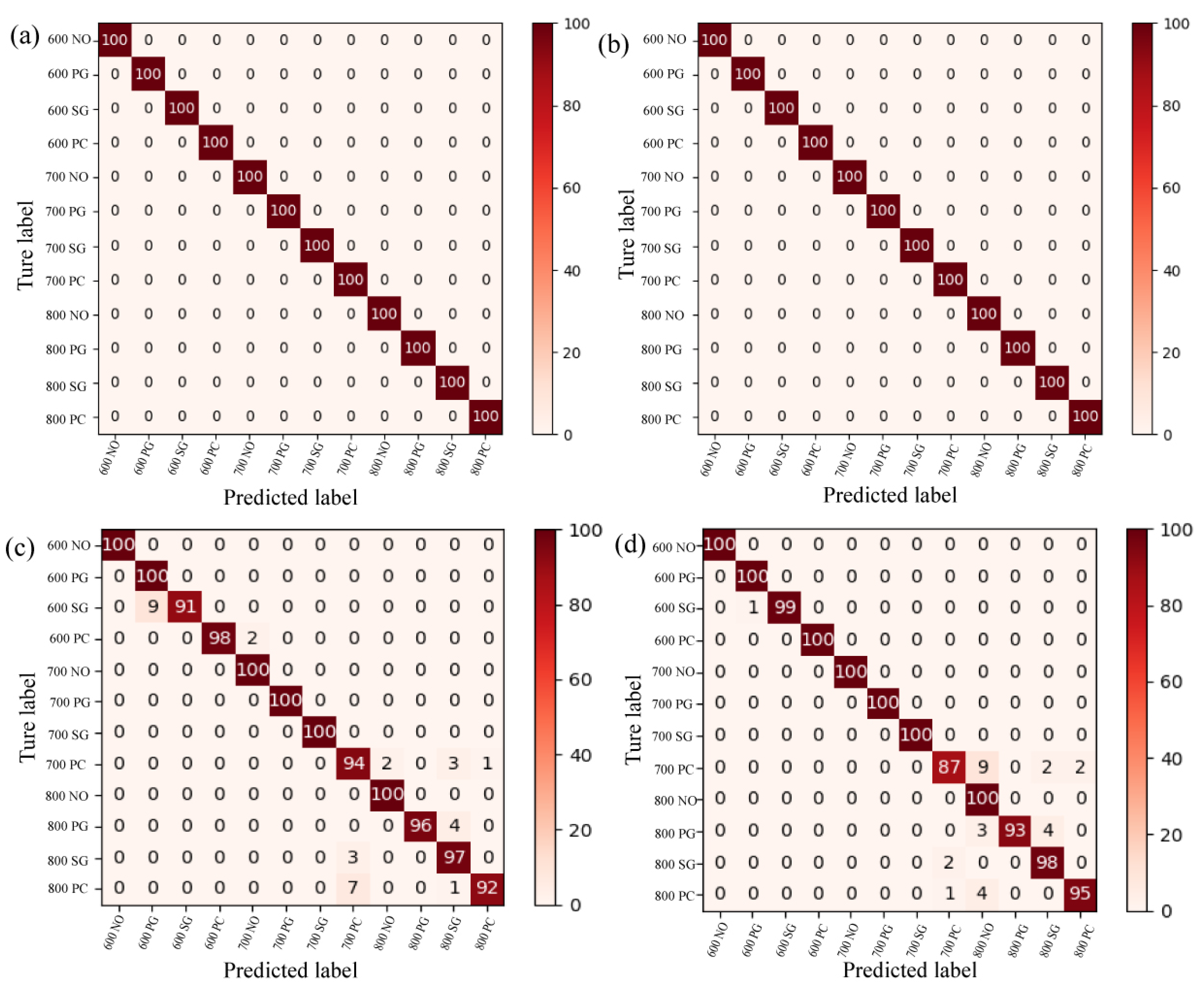
To eliminate the random error, each approach was executed 10 times. Results of four different methods are listed in Table 2. The confusion-matrix plots of the four methods are shown in Figure 6. Evaluation indicators demonstrated that the proposed approach and the CWT could effectively identify the faults of planetary-gear sets, and all evaluation indicators could reach 100%. As can be seen, standard variance was about 0%, which shows that performance was robust. Comparing the confusion matrix of the time domain RP with the artificially selected IMF plots, the true classification number was higher than that of handcrafted features, which concludes that adaptive feature extraction was better than artificially selected features. Therefore, the proposed approach is effective for fault classification of a planetary gearbox under various rotating speeds.
6. Conclusions
In this paper, we proposed a combination of a CNN with recurrence-plot analysis in the angular-domain method for fault classification in planetary gearboxes. The combination of the CNN with the RP was compared with angular domain RP, CWT (cmor4-4), and IMF plots. Even though the CWT could also obtain high valuation accuracy, it needed more epochs. Moreover, due to the speed fluctuations and limitation of handcrafted features, the valuation accuracy of the two other methods was lower than that of the CWT and the proposed method. Finally, experiment results showed that the proposed method is superior to conventional methods on the fault classification of planetary gearboxes.
Author Contributions
Methodology, D.-F.W.; writing—review and editing, X.W., J.N., and G.L.; project administration, Y.G.; funding acquisition, Y.G. All authors have read and agreed to the published version of the manuscript.
Funding
This research was funded by the National Natural Science Foundation of China, grant number 51675251.
Conflicts of Interest
The authors declare no conflict of interest.
Abbreviations
The following abbreviations are used in this manuscript:
| RP | Recurrence plot |
| CNN | Convolutional neural network |
| COT | Computed order tracking |
| AI | Artificial intelligent |
| FFT | Fast Fourier transform |
| CWT | Continuous wavelet transform |
| STFT | Short-time Fourier transform |
| FT | Fourier transform |
| FNN | False nearest neighbors |
| SNR | Signal-to-noise ratio |
| ReLU | Rectified linear unit |
| ADAM | Adaptive moment estimation |
| IMF | Intrinsic mode function |
| EMD | Empirical mode decomposition |
References
- Guo, Y.; Zhao, L.; Wu, X.; Na, J. Vibration separation technique based localized tooth fault detection of planetary gear sets: A tutorial. Mech. Syst. Signal Process. 2019, 129, 130–147. [Google Scholar] [CrossRef]
- Feng, Z.P.; Ma, H.Q.; Zuo, M.J. Amplitude and frequency demodulation analysis for fault diagnosis of planet bearings. J. Sound Vib. 2016, 382, 395–412. [Google Scholar] [CrossRef]
- Guo, Y.; Liu, Q.N.; Wu, X.; Na, J. Gear fault diagnosis based on narrowband demodulation with frequency shift and spectrum edit. Int. J. Eng. Technol. Innov. 2016, 4, 243–254. [Google Scholar]
- Janssens, O.; Slavkovikj, V.; Vervisch, B.; Stockman, K.; Loccufier, M.; Verstockt, S.; de Walle, R.V.; van Hoecke, S. Convolutional neural network based fault detection for rotating machinery. J. Sound Vib. 2016, 377, 331–345. [Google Scholar] [CrossRef]
- Chen, Z.Q.; Li, C.; Sanchez, R.V. Gearbox fault identification and classification with convolutional neural networks. Shock Vib. 2015, 2015, 1–10. [Google Scholar] [CrossRef] [Green Version]
- Yao, Y.; Wang, H.L.; Li, S.B.; Liu, Z.H.; Gui, G.; Dan, Y.B.; Hu, J.J. End-to-end convolutional neural network model for gear fault diagnosis based on sound signals. Appl. Sci. 2018, 9, 1584. [Google Scholar] [CrossRef] [Green Version]
- Lv, Y.; Pan, B.Q.; Yi, C.C.; Ma, Y.B. A Novel Fault Feature Recognition Method for Time-Varying Signals and Its Application to Planetary Gearbox Fault Diagnosis under Variable Speed Conditions. Sensors 2019, 14, 3154. [Google Scholar] [CrossRef] [PubMed] [Green Version]
- Jing, L.Y.; Zhao, M.; Li, P.; Xu, X.Q. A convolutional neural network based feature learning and fault diagnosis method for the condition monitoring of gearbox. Measurement 2017, 111, 1–10. [Google Scholar] [CrossRef]
- Marwan, N.; Romano, M.C.; Thiel, M.; Kurths, J. Recurrence plots for the analysis of complex systems. Phys. Rep. 2007, 438, 237–329. [Google Scholar] [CrossRef]
- Syta, A.; Jonak, J.; Jedliński, Ł.; Litak, G. Failure diagnosis of a gear box by recurrences. J. Vib. Acoust. 2012, 4, 041006–041014. [Google Scholar] [CrossRef]
- Ambrożkiewicz, B.; Guo, Y.; Litak, G.; Wolszczak, P. Dynamical Response of a Planetary Gear System with Faults Using Recurrence Statistics. In Topics in Nonlinear Mechanics and Physics; Springer: Singapore, 2019; pp. 177–185. [Google Scholar]
- Guo, Y.; Wu, X.; Na, J.; Fung, R.F. Envelope synchronous average scheme for multi-axis gear faults detection. J. Sound Vib. 2016, 365, 276–286. [Google Scholar] [CrossRef]
- Fyfe, K.R.; Munck, E.D.S. Analysis of computed order tracking. Mech. Syst. Signal Process. 1997, 11, 187–205. [Google Scholar] [CrossRef]
- Kennel, M.B.; Brown, R.; Abarbanel, H.D.I. Determining embedding dimension for phase-space reconstruction using a geometrical construction. Phys. Rev. A 1992, 45, 3403–3411. [Google Scholar] [CrossRef] [Green Version]
- Cao, L.Y. Practical method for determining the minimum embedding dimension of a scalar time series. Phys. D Nonlinear Phenom. 1997, 110, 43–50. [Google Scholar] [CrossRef]
- Fraser, A.M.; Swinney, H.L. Independent coordinates for strange attractors from mutual information. Phys. Rev. A 1986, 33, 1134–1140. [Google Scholar] [CrossRef] [PubMed]
- Jeong, J.; Gore, J.C.; Peterson, B.S. Mutual information analysis of the EEG in patients with Alzheimer’s disease. Clin. Neurophysiol. 2001, 112, 827–835. [Google Scholar] [CrossRef]
- Thiel, M.; Romano, M.C.; Kurths, J.; Meucci, R.; Allaria, E.; Arecchi, F.T. Influence of observational noise on the recurrence quantification analysis. Phys. D Nonlinear Phenom. 2002, 171, 138–152. [Google Scholar] [CrossRef] [Green Version]
- Gu, J.; Wang, Z.; Kuen, J.; Ma, L.; Shahroudy, A.; Shuai, B.; Liu, T.; Wang, X.X..; Wang, G.; Cai, J.F.; et al. Recent advances in convolutional neural networks. Pattern Recognit. 2018, 77, 354–377. [Google Scholar] [CrossRef] [Green Version]
- Kingma, D.P.; Ba, J. Adam: A method for stochastic optimization. J. Intell. Learn. Syst. Appl. 2014, 10, 121–134. [Google Scholar]
- Sen, A.K.; Longwic, R.; Litak, G.; Górskid, K. Analysis of cycle-to-cycle pressure oscillations in a diesel engine. Mech. Syst. Signal Process. 2008, 2, 362–373. [Google Scholar] [CrossRef]
- Hu, N.Q.; Chen, H.P.; Cheng, Z.; Zhang, L.; Zhang, Y. Fault diagnosis for planetary gearbox based on EMD and deep convolutional neural networks. J. Mech. Eng. 2019, 7, 9–18. [Google Scholar] [CrossRef] [Green Version]
Figure 1.
Combination of convolutional neural network (CNN) and recurrence plot (RP) in angular domain.
Figure 1.
Combination of convolutional neural network (CNN) and recurrence plot (RP) in angular domain.

Figure 2.
Experiment planetary gearbox: (a) test rig; (b) sun gear with tooth-root crack; (c) planet gear with tooth-root crack; (d) planetary carrier with crack.
Figure 2.
Experiment planetary gearbox: (a) test rig; (b) sun gear with tooth-root crack; (c) planet gear with tooth-root crack; (d) planetary carrier with crack.

Figure 3.
Kinematic schema of experiment planetary gearbox.

Figure 4.
Angular-domain recurrence plots: (a) normal (, , ); (b) planet gear-root crack (, , ); (c) sun gear with a tooth-root crack (, , ); (d) planet carrier with crack (, , ).
Figure 4.
Angular-domain recurrence plots: (a) normal (, , ); (b) planet gear-root crack (, , ); (c) sun gear with a tooth-root crack (, , ); (d) planet carrier with crack (, , ).

Figure 5.
CNN detection results with different learning samples. (a) Valuation loss and (b) valuation accuracy.
Figure 5.
CNN detection results with different learning samples. (a) Valuation loss and (b) valuation accuracy.

Figure 6.
Confusion matrix of planetary-gearbox fault classification. (a) Continuous wavelet transform (CWT); (b) angular domain RP; (c) intrinsic mode function (IMF); (d) time domain RP (NO = normal, PG = planet gear, SG = sun gear, PC = planet carrier).
Figure 6.
Confusion matrix of planetary-gearbox fault classification. (a) Continuous wavelet transform (CWT); (b) angular domain RP; (c) intrinsic mode function (IMF); (d) time domain RP (NO = normal, PG = planet gear, SG = sun gear, PC = planet carrier).


Table 1.
Key parameters of selected CNN model.
| Layer | Variable and Dimension | Training Parameters |
|---|---|---|
| Convolutional layer 1 | CW = 5; CH = 5; CN = 32 | Padding = ‘same’ |
| Pooling layer 1 | S = 2 | MaxPooling |
| Convolutional layer 2 | CW = 5; CH = 5; CN = 64 | Drop out = 0.5 |
| Poling layer 2 | S = 2 | MaxPooling |
| Fully connected layer 1 | Nodes = 1024 | Training sample rate = 80% |
| Fully connected layer 2 | Nodes = 512 | Max epoch = 60 |
| Fully connected layer 3 | Nodes = 64 | Learning rate = 0.0001 |
| softmax regression layer | Nodes = 4 | active function = ReLU |
CW = filter width; CH = filter hight; CN = number of filter; S = width of pooling.
Table 2.
Performance results of different methods executed 10 times.
| Evaluation Indicators | Accuracy | Precision | Recall | -Score |
|---|---|---|---|---|
| Time domain RP | 97.2431 ( = 0.838) | 97.4874 ( = 0.603) | 97 ( = 0.84) | 97 ( = 0.863) |
| Angular domain RP | 100 ( = 0) | 100 ( = 0) | 100 ( = 0) | 100 ( = 0) |
| CWT (cmor4-4) | 100 ( = 0) | 100 ( = 0) | 100 ( = 0) | 100 ( = 0) |
| Artificially selected IMF | 97.3266 ( = 3.237) | 97.5712 ( = 2.993) | 97.0833 ( = 3.845) | 97.0833 ( = 3.485) |
Result format is average evaluation indicators (%) ( = standard variance (%)).
© 2020 by the authors. Licensee MDPI, Basel, Switzerland. This article is an open access article distributed under the terms and conditions of the Creative Commons Attribution (CC BY) license (http://creativecommons.org/licenses/by/4.0/).
Share and Cite
MDPI and ACS Style
Wang, D.-F.; Guo, Y.; Wu, X.; Na, J.; Litak, G. Planetary-Gearbox Fault Classification by Convolutional Neural Network and Recurrence Plot. Appl. Sci. 2020, 10, 932. https://doi.org/10.3390/app10030932
AMA Style
Wang D-F, Guo Y, Wu X, Na J, Litak G. Planetary-Gearbox Fault Classification by Convolutional Neural Network and Recurrence Plot. Applied Sciences. 2020; 10(3):932. https://doi.org/10.3390/app10030932
Chicago/Turabian StyleWang, Dan-Feng, Yu Guo, Xing Wu, Jing Na, and Grzegorz Litak. 2020. "Planetary-Gearbox Fault Classification by Convolutional Neural Network and Recurrence Plot" Applied Sciences 10, no. 3: 932. https://doi.org/10.3390/app10030932
Note that from the first issue of 2016, this journal uses article numbers instead of page numbers. See further details here.