
Predictive Machine Learning of Objective Boundaries for Solving COPs


Simula Research Laboratory, Kristian Augusts Gate 23, 0164 Oslo, Norway
*
Author to whom correspondence should be addressed.
AI 2021, 2(4), 527-551; https://doi.org/10.3390/ai2040033
Submission received: 28 September 2021
/
Revised: 22 October 2021
/
Accepted: 24 October 2021
/
Published: 28 October 2021
Abstract
:Solving Constraint Optimization Problems (COPs) can be dramatically simplified by boundary estimation, that is providing tight boundaries of cost functions. By feeding a supervised Machine Learning (ML) model with data composed of the known boundaries and extracted features of COPs, it is possible to train the model to estimate the boundaries of a new COP instance. In this paper, we first give an overview of the existing body of knowledge on ML for Constraint Programming (CP), which learns from problem instances. Second, we introduce a boundary estimation framework that is applied as a tool to support a CP solver. Within this framework, different ML models are discussed and evaluated regarding their suitability for boundary estimation, and countermeasures to avoid unfeasible estimations that avoid the solver finding an optimal solution are shown. Third, we present an experimental study with distinct CP solvers on seven COPs. Our results show that near-optimal boundaries can be learned for these COPs with only little overhead. These estimated boundaries reduce the objective domain size by 60-88% and can help the solver find near-optimal solutions early during the search.
1. Introduction
Constraint Optimization Problems (COPs) are commonly solved by systematic tree search, such as branch-and-bound, where a specialized solver prunes those parts of the search space with a worse cost than the current best solution. In Constraint Programming (CP), these systematic techniques work without prior knowledge and are steered by the constraint model. However, the worst-case computational cost to fully explore the search space is exponential, and the search performance depends on the solver configuration, such as the selection of the right parameters, heuristics, and search strategies, as well as appropriate formulations of the constraint problems to enable efficient pruning of the search space.
Machine Learning (ML) methods, on the other hand, are data-driven and are trained with labeled data or by interaction with their environment, without explicitly considering the problem structure or any solving procedure. At the same time, ML methods can only approximate the optimum and are therefore not a full alternative. The main computational cost of these methods lies in their training, but the cost when estimating an outcome for a new input is low. This low inference cost makes ML an interesting candidate for integration with the more costly tree search. Previous research has examined this integration to several extents, albeit selecting the appropriate algorithm within a solver and configuring it for a given instance, learning additional constraints to model a problem, or learning partial solutions.
In this paper, we provide an overview of the body of knowledge on using ML for CP. We focus on approaches where the ML model is trained in a supervised way from existing problem instances with solutions and the collected information gathered while solving them. We discuss the characteristics of supervised ML and CP and how to use predictive ML to improve CP solving procedures. A graphical overview of predictive ML applications for CP is shown in Figure 1.
The second part of the paper discusses a boundary estimation method called Bion, which combines logic-driven constraint optimization and data-driven ML, for solving COPs. An ML-based estimation model predicts boundaries for the objective variable of a problem instance, which can then be exploited by a CP solver to prune the search space. To reduce the risk of inaccurate estimations, which can render the COP unsatisfiable, the ML model is trained with an asymmetric loss function and adjusted training labels. Setting close bounds for the objective variable is helpful to prune the search space [1,2]. However, estimating tight bounds in a problem- and solver-agnostic way is still an open problem [3]. Such a generic method would allow many COP instances to be solved more efficiently. Our method was first introduced in [4], where an initial analysis of the results led us to conclude that Bion was a promising approach to solve COPs. Here, we revisit and broaden the presentation of Bion in the general context of predictive machine learning for constraint optimization. We extend our experimental evaluation analysis and show that boundary estimation is effective to support COP solving.
Bion is a two-phase procedure: first, an objective boundary for the problem instance is estimated with a previously trained ML regression model; second, the optimization model is extended by a boundary constraint on the objective variable, and a constraint solver is used to solve the problem instance. This two-phase approach decouples the boundary estimation from the actual solver and enables its combination with different optimized solvers. Training the estimation model with many problem instances is possible without any domain or expert knowledge and applies to a wide range of problems. Solving practical assignment, planning, or scheduling problems often requires repeatedly solving the very same COP with different inputs. Bion is well fitted for these problems, where training samples, which resemble realistic scenarios, can be collected from previous iterations. Besides, for any COP, Bion can be used to pretrain problem-specific ML models, which are then deployed to solve new instances.
The remainder of this paper is structured as follows. In Section 2, we discuss the necessary background for the integration of predictive ML and CP, including the data curation and preparation of problem instances to be usable in ML. Section 3 reviews existing work on predictive ML and CP for algorithm selection and configuration, constraint learning, and learning to solve. Afterwards, we introduce Bion in Section 4, an ML-based method to estimate the boundaries of the objective variable of COPs as a problem- and solver-independent method tool to support constraint optimization solvers. We discuss training techniques to avoid inaccurate estimations and compare various ML models such as gradient tree boosting, support vector machine, and neural networks, with symmetric and asymmetric loss functions. A technical CP contribution lies in the dedicated feature selection and user-parameterized label shift, a new method to train these models on COP characteristics. In Section 5, Bion’s ability to prune objective domains, as well as the impact of the estimated boundaries on solver performance are evaluated on seven COPs that were previously used in the MiniZinc challenges to compare CP solvers’ efficiency. Finally, Section 6 concludes the paper with an outlook on future applications of predictive ML to CP.
2. Background
This section presents a background discussion on constraint optimization and supervised machine learning. We introduce the necessary terminology and foundations under the context of predictive ML for CP. For an in-depth introduction beyond the scope of this paper, we refer the interested reader to the relevant literature in constraint optimization [5,6] and machine learning [7,8,9].
2.1. Constraint Optimization Problems
Throughout this paper, constraint optimization is considered in the context of constraint programming over finite domains [5]. In that respect, every variable of an optimization problem is associated with a finite set of possible values, called a Finite Domain (FD) and denoted . Each value is associated with a unique integer without any loss of generality, and thus, , where (resp. ) denotes the lower (resp. upper) bound of . Each variable takes one, yet unknown value in its domain, i.e., and , even if not all the values of are necessarily part of .
A constraint is a relation among a subset of the decision variables, which restrain the possible set of tuples of values taken by these variables. In constraint programming over FD, different types of constraints can be considered, including arithmetical, logical, symbolic, or global relations. For instance, is an arithmetical constraint, while , where (resp. ) stands for true (resp. false), is a logical constraint. Symbolic and global constraints include a large panel of nonfixed length relations such as all_different, which constrains each variable to take a different value, element, which enforces the relation , where and can all be unknowns. More details and examples can be found in [5,6].
Definition 1
(Constrained Optimization Problem (COP)). A COP is a triple where denotes a set of FD variables, called decision variables, denotes a set of constraints, and denotes an optimization function, which depends on the variables of . ’s value ranges in the domain of the variable ( in ), called the objective variable.
Solving a COP instance requires finding a variable assignment, i.e., the assignment of each decision variable to a unique value from its domain, such that all constraints are satisfied and the objective variable takes an optimal value. Note that COPs have to be distinguished from well-known Constraint Satisfaction Problems (CSPs) where the goal is only to find satisfying variable assignments, without taking care of the objective variable.
Definition 2
(Feasible/optimal solutions). Given a COP instance , a feasible solution is an assignment of all variables in their domain, such that all constraints are satisfied. denotes the value of objective variable for such a feasible solution. An optimal solution is a feasible solution that optimizes the function to the optimal objective value .
Definition 3
(Satisfiable/unsatisfiable/solved COP). A COP instance is satisfiable (resp. unsatisfiable) iff it has at least one feasible solution (resp. no solution). A COP is said to be solved if and only if at least one of its optimal solutions is provided.
Solving a COP instance can be performed by a typical branch-and-bound search process, which incrementally improves a feasible solution until an optimal solution is found. Roughly speaking, in the case of minimization, branch-and-bound works as follows: starting from an initial feasible solution, it incrementally adds to the constraint , such that any later found feasible solution has necessarily a smaller objective value than the current value. This is helpful to cut the search tree of all feasible solutions that have a value equal to or larger than the current one. If there is no smaller feasible value and all possible variable assignments have been explored, then the current solution is actually an optimal solution. Interestingly, the search process can be time-controlled and interrupted at any time. Whenever the search process is interrupted before completion, it returns as the best feasible solution found so far by the search process, i.e., a near-optimal solution. This solution is provided with neither the proof of optimality nor the guarantee of proximity to an optimal solution, but it is still sufficient in many applications.
This branch-and-bound search process is fully implemented in many Constraint Programming (CP) solvers. These solvers provide a wide range of features and heuristics to tune the search process for specific optimization problems. At the same time, they do not reuse any of the already-solved instances of a constraint problem to improve the optimization process for a new instance. In addition to presenting existing works on predictive learning for constraint optimization, this paper proposes a new method to reuse existing known boundaries to nurture a machine learning model to improve the optimization process for a new instance.
2.2. Supervised Machine Learning
At the core of the predictive applications described in this paper, a supervised ML model is trained and deployed. In supervised machine learning, the model is trained from labeled input/output examples to approximate the underlying, usually unknown function.
Definition 4
(Supervised machine learning). Given a set of training examples , a supervised machine learning model approximates a function , with X being the input space and Y being the output space. Here, is a vector of instance features and is the corresponding label, representing the target value to be predicted.
Every value in x corresponds to a feature, that is a problem instance characteristic that describes the input to the model. In most cases, the input consists of multiple features and is also described as the feature vector. The output of the model, , is defined as a vector, as well, although it is more common to have a model that only predicts a single value. This is the case in regression problems, when predicting a continuous value, or binary classification, when deciding whether to activate a functionality or not.
The model P is trained from a training set, consisting of example instances . Training the model describes the process to minimize the error between the estimated value and the true (observed) value y of the training examples. The error is assessed with a loss function, which can be different depending on the task of the machine learning model. We show examples for two commonly used types of loss functions. For regression problems, where a continuous output value is estimated, the loss is assessed via the mean-squared error. In classification, where the input is assigned to one of multiple classes, the cross-entropy loss is calculated.
Definition 5
(Mean-Squared Error (MSE)). Given a set of N estimated and observed target values , the MSE is calculated as:
Within the calculation of MSE, positive and negative errors have the same effect, but larger errors are more strongly penalized, i.e., they have a larger influence, than smaller errors.
Definition 6
(Cross-entropy loss). Given a set of N estimates and K classes, the cross-entropy (also log-likelihood) is calculated as:
with being the probability of belonging to class k and:
An example for the training scheme is shown in Figure 2 for a linear regression model. The weights of the linear function are adjusted such that the total error between estimated and true values is minimized. In the given example, the training examples do not strictly follow a linear trend and are therefore difficult to approximate with only a small error. This is an indicator to use a more complex model for better results and to describe the output via different features than only x, if possible.
2.3. Machine Learning Models
Many supervised ML models exist and have been shown to be applicable to a wide range of problems. However, there is no one best model, and depending on the application, different models can show good performance.
In this section, we introduce five widely used machine learning models for the application in predictive ML for CP: gradient tree boosting, neural network, support vector machine, k-nearest neighbors, and linear regression. We briefly discuss each model and highlight relevant characteristics for applying them to constraint problems.
2.3.1. Gradient Tree Boosting
Gradient Tree Boosting (GTB), also gradient boosting machine, is an ensemble method where multiple individual weak models, whose error rate slightly outperforms random guessing, are combined into a strong learner [10]. At each iteration, additional weak models are trained on a modified subset of data to add information to the previous prediction. The individual weak models in GTB are decision trees, which by themselves have weak estimation accuracy compared to other models, but are robust to handle different types of inputs and features [7] (Ch. 10).
2.3.2. Neural Network
A multilayer Neural Network (NN) approximates the function to be learned over multiple layers of nodes or neurons. Neural networks can be applied to different problems, e.g., classification or regression, especially when there is a large amount of training data. Designing a neural network requires selecting an architecture and the number of layers and nodes, as well as performing a careful hyperparameter optimization to achieve accurate results [8].
An ensemble of multiple NNs can be formed to reduce the generalization error of a single NN [11], by taking the average of all predictions. As errors are expected to be randomly distributed around the actual value, an ensemble can reduce the error.
2.3.3. Support Vector Machine
Support Vector Machines (SVMs) map their inputs into a high-dimensional feature space. This feature space is defined by a kernel function, which is a central component. Once the data have been mapped, linear regression is performed in this high-dimensional space [12]. One common variant for regression problems is -SVR, which is usually trained using a soft margin loss [13]. Under soft margin loss, an error is penalized only if it is larger than a parameter ; otherwise, it is similar to a squared error function. Having the additional margin of allowed errors avoids minimal adjustments during training and allows for higher robustness of the final model.
2.3.4. Nearest Neighbors
Nearest neighbor methods, also k-Nearest Neighbors (kNNs) or neighbors, relate an unseen instance to the closest samples, i.e., the nearest neighbors, in the training set [14]. The distance between points is calculated from a distance metric, which is often the Euclidean distance. In the case of k-nearest neighbors, the number of neighbors to consider is fixed to k, which is usually a small integer value. Other methods set the number of neighbors dynamically from the data density in the training set and a threshold for the maximum distance. For regression problems, the estimated value y is calculated by a weighted average over the neighbors’ values. The weights are either uniform or proportional to the distance.
Nearest neighbor methods have the advantage of being simple and nonparameterized, i.e., they do not require a training phase, but a complete training is necessary to process new instances. Because searching through all training samples for each estimation is inefficient for a large training set, tree-based data structures can be used to organize the data for faster access, for example K-D trees [15] or ball trees [16].
2.3.5. Linear Regression
Linear Regression (LR) is a simple statistical approach to find a linear relationship between a set of input features and the target value. Applying linear regression is effective in scenarios where a linear relationship can be assumed. In other scenarios, LR is less accurate than the other introduced methods. However, because it is easy to train and apply, LR is commonly used as a baseline method to identify and justify the need for more complex, nonlinear methods in ML applications.
The model is formed by the linear relationships between each of the n features and the target value, the dependent variable y. This relationship is captured by the parameter for each feature : . Linear regression is trained via the ordinary least squares method [7] (Ch. 3), an iterative method to minimize the squared error between the estimated and true target.
2.4. Data Curation
Machine learning methods are data-driven and need a data corpus to be trained, before they can be used to make estimations on new instances. In this section, we discuss the collection of a data corpus, its organization for training the model, and the preprocessing to transform the data into a format that is usable as the model input.
2.4.1. Collection
A sufficient amount of training data is the basis to train a supervised ML model. Data for CSPs and COPs, that is problem instances, can either be downloaded from open repositories for existing constraint problems, collected from historical data, or synthetically generated.
For many problems, constraint models and instances can be freely accessed from online repositories. The CSP library (CSPLib) [17] contains a large collection of constraint models, instances, and their results in different modeling languages. Furthermore, problem-specific libraries exist, such as TSPLib [18] for the traveling sales person problem and related problems or ASLib [19] for algorithm selection benchmarks. Finally, there are repositories of constraint models and instances in language-specific repositories, for example in MiniZinc (online at: https://github.com/MiniZinc/minizinc-benchmarks, accessed 26 September 2021) or XCSP3 (online at: http://www.xcsp.org/).
Having a generator allows us to create a large training corpus for a particular problem, but this also requires additional effort to develop the generator program. This solution might not be suitable in all cases. Another approach is to generate instances directly from the constraint model [20]. The constraint model is reformulated by defining the given instance parameters as variables to be found by the solver. Solving this reformulation with random value assignment then leads to a satisfiable problem instance of the original constraint model.
However, for all generators, the difference between generated instances, which are distributed over the whole possible instance space, and realistic instances, which might only occupy a small niche of the possible instance space, has to be considered by either adjusting the generator to create realistic instances or to ensure the training and test set include realistic instances from other sources.
2.4.2. Data Organization
Data used to build an ML model are split into three parts: (a) the training set, (b) the development (dev) or validation set, and (c) the test set. The training set is used to train the model via a learning algorithm, whereas the dev set is only used to control the parameters of the learning algorithm. The test set is not used during training or to adjust any parameters, but only serves to evaluate the performance of the trained model. Especially the test set should be similar to those instances that are most likely to be encountered in practical applications.
The training set holds the largest part of the data, ranging from 50–80% of the data, while the rest of the data are equally divided between the validation and test sets. This is a rough estimate, and the exact split is dependent on the total size of the dataset. In any case, it should be ensured that the validation and test sets are sufficiently large to evaluate the trained model.
2.4.3. Representation
The representation refers to the format into which a problem instance is transformed before it can be used as an ML input. An expressive representation is crucial for the design of an ML model with a high influence on its later performance. Representation consists of feature selection and data preparation, which are introduced in the following.
Feature Selection
Feature selection defines which information is available for the model to make predictions, and if insufficient or the wrong information is present, it is not possible to learn an accurate prediction model, independent of the selected machine learning technique. A good feature selection contains all features that are necessary to calculate the output and captures relations between instance data and the quantity to estimate.
As a long-term vision, it is desirable to learn a model end-to-end, that is from the raw COP formulation and instance parameters, without having to extract handcrafted features. Currently, most machine learning techniques work with fixed, numerical input and output vectors. There are machine learning techniques capable of handling variable-length inputs and outputs, for example recurrent neural networks such as LSTM [21], but these have, to the best of our knowledge, not yet been successfully applied in the area of predictive ML for CP and will not be further discussed here. Instead, we focus on the common case of handcrafting a fixed-size feature vector.
For the selection of features, we first need to consider the application of the machine learning model. Is it a problem-specific application, which handles only instances of one defined optimization problem, or is it a problem-independent application, which handles instances of many different optimization problems?
In COP-specific applications, domain knowledge can be exploited. For example, when building a predictive model for the Traveling Sales Person (TSP) problem [22], features describing the spatial distribution of the cities and the total area size are valuable [23]. Similarly, the Constrained Vehicle Routing Problem (CVRP) has been investigated to identify problem-specific features that are beneficial to reason over the solution quality [24] or aid the search process [25,26,27].
Without domain knowledge, more generic features have to be used to capture the characteristics and variance of different constraint models and their instances. One approach is the design of portfolio solvers, where a learning model is used to decide which solver to run for a given problem instance [28,29,30,31,32,33]. Feature extraction exploits the structure of the general constraint model and the specific instance, its constraints and variables, and their domains. Features are further categorized as static features, which are constant for one model and instance, and dynamic features, which change during the search and are therefore especially relevant for algorithm configuration and selection tasks. As a representative explanation, Table 1 shows an overview of features to describe problem instances. While many of these features are constant for multiple instances of the same constraint problem, e.g., the number of constants or which constraints were defined, the variables and their domains depend on the instance parameters and can offer descriptive information that discriminate several instances of the same problem.
Several studies have been performed to analyze the ability of these generic features to characterize and discriminate COP characteristics [19,36,37,38]. Their main conclusion was that a small number of features can be sufficient discriminators, but that there is no single set of best features for all constraint problems used in their experiments. An approach to overcome this issue is therefore to start with a larger set of features than practically necessary and perform dimensionality reduction (see the next section for a detailed explanation) to remove features with little descriptive information.
Data Preparation
Once the features are selected and retrieved, the next step is to preprocess the data, such that they can be used by the machine learning model, by performing dimensionality reduction and scaling.
A dimensionality reduction step can shrink the size of the feature vector. Reducing the dimensionality, which means having less model inputs, can thereby also reduce the model complexity. Features that are constant for all instances are removed, as well as features that only show minimal variance below a given threshold. Other dimensionality reduction techniques, e.g., Principal Component Analysis (PCA), apply statistical procedures to reduce the data to a lower-dimensional representation while preserving its variance. These reduction techniques can further reduce the number of features, but with the downside that it is no longer possible to directly interpret the meaning of each feature.
Feature scaling is necessary for many models and means to transform the values of each feature, which might be in different ranges, into one common range. Scaled features reduce model complexity as it is not necessary to have the weights of a model account for different input ranges. One common technique is to scale the feature by subtracting its mean and dividing by the standard deviation, which transforms the features to approximately resemble a normal distribution with zero mean and unit variance. Another technique is called minmax-normalization and scales the feature based on the smallest and largest occurring values, such that all values are scaled into the range .
Note that it is important to keep track of how each preparation step is performed on the training set, as it has to be repeated in the same way on each new instance during testing and production. This means the feature vector of a new instance contains the same features and each feature is scaled by the same parameters, e.g., it is scaled by the training set’s mean and standard deviation.
3. Predictive Machine Learning for Constraint Optimization
The opportunities for the integration of predictive ML in constraint programming are vast and relevant in several research directions [39]. We first look at general categorizations and approaches to the combination of predictive ML and CP, before we discuss the body of knowledge in specialized research areas.
A recent work by [40] introduced a general framework for the integration of ML and CP, called the Inductive Constraint Programming loop (ICP) [40]. The framework is based on threemain building blocks: a CP component, an ML component, which can be controlled, as well as an external world, which cannot be controlled and which produces observations. All these building blocks are interconnected and can receive and provide information from and to each other, e.g., the CP component receives new constraint problems via a world-to-CP relation and returns solutions via a corresponding apply-to-world relation. An overview of the ICP framework and all defined relations is shown in Figure 3. The majority of predictive machine learning applications for CP can be embedded into the ICP framework, as they exploit the ML-to-CP relation, where the ML model transfers information to the component, which is their main purpose. Furthermore, these applications also exploit the opposite CP-to-ML relation to return feedback from the solver, e.g., runtimes, found solutions, to the ML model for improvement.
Reference [41] presented a general framework for embedding ML-trained models in optimization techniques, called empirical model learning [41]. The approach deploys trained ML models directly in the COP as additional global constraints. Experimental results showed that the embedded empirical ML model can improve the total solving process. The proposed integration further leads to easier deployment of the trained ML model and to reducing the complexity of the setup, but, at the same time, the complexity of the model itself is increased as compared to the pure COP.
3.1. Algorithm Selection and Configuration
The area of algorithm selection and configuration applies predictive ML to analyze individual problem instances and decide the most appropriate solver, its heuristic, or the setting of certain tuning parameters of a solver. All these techniques have in common that they work on a knowledge base that is mostly not restricted to a single constraint optimization problem, but applicable to instances from many different problems. Furthermore, these approaches affect changes on the solver, but do not modify or adjust the constraint problem or the problem instance.
Algorithm selection within a constraint solver can be used to decide which search strategy to use. A search strategy consists of a variable selection, that is which variable will next have a value assigned, and a value selection, that is which value is assigned to the variable. Reference [42] proposed a classification model to select from up to eight different heuristics, consisting of both variable and value selection [42]. The search strategy is repeatedly selected during the search, e.g., upon backtracking, to be able to adapt to the characteristics of the problem instance in different regions of the search space. The machine learning model uses an SVM (see Section 2.2) and a set of 57 features to describe an instance.
In [43], this work was extended to a life-long learning constraint solver, whose inner machine learning model was repeatedly retrained based on newly encountered problem instances and the experiences from selected search heuristics. The methodology was refined to select a heuristic for a predefined checkpoint window, i.e., a heuristic was fixed for a sequence of decisions, before the next heuristic was selected. In total, 95 features were involved, describing static features, such as the problem definition, variable and constraint information, dynamic features to monitor the search performance.
Similarly, Reference [44] classified problem instances to decide whether solving them benefits from lazy learning, an effective but costly CSP search method [44]. They analyzed the primal graph of the instance to extract instance features. The primal graph represents every variable as a node, and variables that occur in the scope of a constraint are connected via edges. Using this graph structure allows extracting features su9ch as the edge density, graph width, or the proportion of constraints that share the same variable.
Ref. [45] investigated methods to learn a value selection heuristic [45]. As part of their work, they discussed the problem of gathering samples to train the ML model. Ideally, one would require exactly solved instances, but in practice, this incurs a high computational cost for every training instance. Their approach was to define an alternative scoring function to be used as the training target. This scoring function was chosen such that it did not require exact solving of the instance, and therefore, gathering the training data was less expensive overall.
Besides supervised ML techniques, adaptive ML methods, such as reinforcement learning, are also applied to configure search algorithms and their parameters, e.g., in large neighborhood search [46] or to select tree search heuristics [47].
Reliable information about expected runtimes for an algorithm on a problem instance can be helpful not only for algorithm selection and configuration, but further for selecting hard benchmark instances that distinguish different algorithms and to analyze the hardness properties of the problem classes [22]. Reference [22] proposed empirical performance models (EPMs) for runtime prediction. These EPMs use a set of generic and problem-specific features to model the runtime characteristics. Another study on runtime prediction for TSP was published in [48], where the authors defined a set of 47 TSP-specific features to assess instance hardness and algorithm performance. For a comprehensive overview of the literature on runtime prediction, we refer the interested reader to [22].
The previously discussed work considered algorithm configuration and selection within one solver to optimize its performance. As mentioned earlier, other approaches are focused towards combining multiple distinct solvers into a portfolio solver [33]. Using machine learning and heuristics, the planning component of the portfolio solver determines the execution schedule of the solver [30,31]. In the case of parallel portfolio solvers, a subset of solvers is run in parallel until a solution is found or, if the optimal solution is wanted, it can exchange information about intermediate solutions found during the search, e.g., sharing the best found objective bound [49]. Popular portfolio solvers include SATZilla [28], CPHydra [29], Sunny-CP [50], or HaifaCSP [51].
3.2. Constraint Learning
During the last decade, considerable progress has been made in the field of automatic constraint learning. Starting from a dataset of solution and nonsolution examples, several approaches have been proposed to extract constraint models fitting the data. Pioneering this question, the ICON European project explored different approaches to this problem. It is worth noting that these approaches to learn in CP are different from the previously described usages of predictive ML to CP, as, unlike statistical ML, the learning model is based on logic-driven approaches, which extract an exact model from examples. Nevertheless, constraint learning approaches can be used to define predictive models to support other constraint models as well and are therefore included here also.
In [52,53], Beldiceanu and Simonis proposed ModelSeeker, an approach that returns the best candidate global constraint representing a pattern occurring in a set of positive examples. Following initial research ideas published in [54], Reference [54] subsequently developed constraint acquisition as a strong inductive constraint learning framework [55,56,57]. Starting from sequences of integers representing solutions and nonsolutions, constraint acquisition progressively refines an admissible and maximal model, which accommodates all positive and negative examples. In [58,59], Reference [58] already proposed a constraint acquisition method based on inductive logic programming where both positive and negative examples can be handled, but the method captured the constraint network structure using some input background knowledge. Constraint acquisition is independent of any background knowledge and just requires a bias, namely a subset of a constraint language, to be given as the input. Interestingly, these constraint learning approaches are all derived from initial ideas developed in Inductive Logic Programming (ILP) [60]. The framework developed in this paper does not originate from ILP and does not try to infer a full CSP or constraint optimization model from sequences of positive and negative examples. Instead, it learns from existing solved instances to acquire suggested boundaries for the optimization variables. In that respect, it can complement constraint acquisition methods by exploiting solved instances and not only solutions and nonsolutions.
3.3. Learning to Solve
Applications and research on predictive ML for CP are sometimes classified as learning to solve, putting an emphasis on the ML component and its contribution to CP. This terminology is especially present in research that focuses on learning to solve optimization problems without the need for an additional solver [61,62,63,64,65]. Connected to the development of deep learning techniques, these approaches are able to solve small instances of constraint problems, but are not competitive with respect to the capabilities of state-of-the-art constraint solvers. A recent survey on the usage of reinforcement learning for combinatorial optimization can be found in [66].
4. Estimating Objective Boundaries
In this part of the paper, we present one application of predictive machine learning for constraint optimization, namely Bion, a novel boundary estimation technique. Boundary estimation supports the constraint solver by adding additional boundaries on the objective of a problem instance. The objective boundaries are estimated via a machine learning model, which has been trained on previously solved problem instances. Through the additional constraints, the search space of the constraint problem is pruned, which again allows finding good solutions early during the search.
In general, exact solvers already include heuristics to find feasible initial solutions that can be used for bounding the search [67]. For example, some CP and MIP solvers use LP relaxations of the problem to find the boundary. Other CP solvers rely on good branching heuristics and constraint propagation to find close bounds early [5]. These approaches are central to the modus operandi of the solvers and crucial for their performance. Boundary estimation via predictive ML runs an additional bounding step before executing the solver and uses an ML-based heuristic, which is learned from historical data to already bound the objective and search space of the COP instance.
With boundary estimation, a different approach to COP solving is taken. The CP solver exploits the constraint structure of a COP and considers only the current instance. In contrast, we train the ML model, which we refer to as the estimator, on the structure of instance parameters and the actual objective value from example instances. Thus, it only indirectly infers the model constraints, but it is not explicitly made aware of them. Our approach combines data- and logic-driven approaches to solve COPs and benefits from the estimation provided by the data-driven prediction and also the optimal solution computed by the logic-driven COP solver. In principle, Bion boosts the solving process by reducing the search space with estimated tight boundaries on the optimal objective.
We now introduce the concept of estimated boundaries, which refers to providing close lower and upper bounds for the optimal value of .
Definition 7
(Estimation). An estimation is a domain that defines boundaries for the domain of . The domain boundaries are predicted by a supervised ML model , that is .
Definition 8
(Admissible/inadmissible estimations). An estimation is admissible iff . Otherwise, the estimation is said to be inadmissible.
We further classify the two domain boundaries as cutting and limiting boundaries in relation to their effect on the solver’s search process. Depending on whether the COP is a minimization or maximization problem, these terms refer to different domain boundaries.
Definition 9
(Cutting boundary). The cutting boundary is the domain boundary that reduces the number of reachable solutions. For minimization, this is the upper domain boundary ; for maximization, this is the lower domain boundary .
Definition 10
(Limiting boundary). The limiting boundary is the domain boundary that does not reduce the number of reachable solutions, but only reduces the search space to be explored. For minimization, this is the lower domain boundary ; for maximization, this is the upper domain boundary .
For the sake of simplicity, in the rest of the paper, we focus exclusively on minimization problems; however, Bion is similarly applicable to maximization problems.
4.1. Optimization with Boundary Constraints
We first present the full process to solve a COP with Bion, which receives as inputs both an optimization model, describing the problem in terms of the variables and constraints , and its instance parameters, which include data structure sizes, boundaries, and constraint parameters. The COP is the same for all instances; only the parameters given as a separate input can change. The process of solving COPs with an already trained estimator is shown as a pseudocode formulation in Algorithm 1. For the simplicity of the formulation, we represent the static COP and the instance parameters merged into one triple .
| Algorithm 1 Pseudocode formulation for the COP solving process with Bion. |
|
Boundary estimation adds a preprocessing step to COP solving, as well as a rule for handling unsatisfiable instances. During preprocessing, the current problem instance is analyzed and the trained estimator estimates a boundary on the objective value of this specific instance. To provide the estimated boundary, instance-specific features are extracted from the COP model and its instance parameters. These features serve as the input of the estimator, which returns the estimated boundary value.
Afterwards, Bion adds the boundary value as an additional constraint on the objective variable to the optimization model. The extended, now instance-specific model and the unmodified instance parameters are then given to the solver. If the solver returns a solution, the process ends, as the problem is solved. However, if the approximated objective value is too low, i.e., the estimation is inadmissible, it can render the problem unsatisfiable. In this case, Bion restarts the solver with the inverted boundary constraint, such that the estimation is a lower bound on . If the COP is now satisfiable, the estimation is inadmissible. Otherwise, unsatisfiability is due to other reasons. When the COP is solved, both the input and the objective value are stored for future training of the estimator.
4.2. Feature Selection
Each COP consists of constraints, variables, and their domains. To use these components as estimator inputs, it is necessary to extract and transform features that describe a problem and its data in a meaningful way. As we discussed, a good set of features captures relations between instance data and the quantity to estimate, i.e., the objective value. Furthermore, the features are dynamic in terms of the individual variability of an instance, but static in the number of features, that is each instance of one problem is represented by the same features.
Among the various types of variable structures one can find in COPs, nonfixed data structures such as arrays, lists, or sets are the main contributors of variability and of major relevance for feature selection. For each of these data structures, nine common metrics from the main categories of descriptive statistics are calculated to gather an abstract, but comprehensive description of the contained data: (1) the number of elements, including the (2) minimum and (3) maximum values. The central tendency of the data is described by both the (4) arithmetic mean and (5) median and the dispersion by the (6) standard deviation and (7) interquartile range. Finally, (8) skewness and (9) kurtosis describe the shape of the data distribution. Scalar variables are each added as features with their value.
The constraints of a model are fixed for all instances, but due to different data inputs, the inferred final models for each problem instance differ. To capture information about the variables generated during compilation and model-specific information, we used 95 features as implemented in the current version of mzn2feat [34], which are listed in Table 2. Several of these features have the same value for all instances as they capture static properties of the COP, but some add useful information for different instances, which supports the learning performance. Nevertheless, preliminary experiments showed that including the nonstatic features of the constraint model improved the estimation accuracy.
In general, all features can have varying relevance to express the data, depending on the model and the necessary input. However, as Bion was designed to be problem-independent, the same features are at first calculated for all problems. During the data preprocessing phase of the model training, all features with zero variance, that is the same value for all instances, are removed to reduce the model complexity. Each feature is further standardized by subtracting the mean and dividing by the standard deviation.
4.3. Avoiding Inadmissible Estimations
One main risk, when automatically adding constraints to a COP, is to render the problem unsatisfiable. In the case of boundary estimation, an inadmissible estimation below the optimum value prohibits the solver from finding any feasible solution. Even though this is often detected early by the solver, there is no guarantee, and thus, it is necessary to tame this issue. To mitigate the risk, three countermeasures were considered in the design of Bion.
First, during COP solving with Bion, unsatisfiable instances provide information about the problem and allow us to restart the solver with an inverted boundary constraint, such that an upper bound becomes a lower bound; second, training the estimator with an asymmetric loss function penalizes errors on the side of inadmissible underestimates more strongly than admissible overestimates, and thereby discourages misestimations; third, besides exploiting the training error, the estimator is explicitly trained to overestimate. This requires adjusting the training label from the actual optimal objective value towards an overestimation.
4.3.1. Symmetric vs. Asymmetric Loss
Common loss functions used for training ML models, such as the MSE, are symmetric and do not differentiate between positive or negative errors. An asymmetric loss function, on the other hand, assigns higher loss values for either underestimations or overestimations, which means that certain errors are more penalized than others. Figure 4 shows an example of quadratic symmetric and asymmetric loss functions.
The shifted squared error loss is an imbalanced variant of squared error loss. The parameter a shifts the penalization towards underestimation or overestimation and influences the magnitude of the penalty. Formally speaking,
Definition 11
(Shifted Squared Error Loss).
where is the estimated value and y is the true target value and a is a parameter that shifts the penalization towards underestimation or overestimation.
In Section 5, we compare the usage of both symmetric and asymmetric loss functions plus label shift to evaluate the importance of adjusting model training to the problem instances.
4.3.2. Label Shift
Boundary estimation only approximates the objective function of the COP, which means there is no requirement on the convergence towards a truly optimum solution. Said otherwise, Bion can accept estimation errors after training. This allows Bion to work with fewer training examples than what could be expected with a desired exact training method. This is appropriate here, as collecting labeled data requires solving many COP instances first, which can be very costly.
However, there is a risk that the trained model underestimates (in the case of minimization) the actual objective value. Such an inadmissible estimation, as defined above, leads to an unsatisfiable constraint system and prohibits the COP solver from finding any feasible solution. On the other hand, a too loose, but admissible overestimation may not sufficiently approximate the actual optimum. To address this risk, we introduced label shift in Bion, which adjusts the training procedure with one user-controlled parameter. Label shift is similar to the concept of prediction shift described in [68], but based on the specific COP model.
Definition 12
(Label Shift).
where is the upper bound of the objective domain, y is the optimal objective value of the training instance, and is the adjusted label for training the estimator, as the result of the label shift adjustment. Label shift depends on λ, which is an adjustment factor to shift the target value y between the domain boundary and the actual optimum. The trade-off between a close and admissible estimation and an inadmissible estimation is thus controlled by the value of λ.
4.4. Estimated Boundaries during Search
Using Bion to solve a COP consists of the following steps:
- (1)
- (Initially) Train an estimator model for the COP;
- (2)
- Extract a feature vector from each COP instance;
- (3)
- Estimate both a lower and an upper objective boundary;
- (4)
- Update the COP with the estimated boundaries;
- (5)
- Solve the updated COP with the solver.
The boundaries provided by the estimator can be embedded as hard constraints on the objective variable, i.e., by adding . The induced overhead is negligible, but dealing with misestimations requires additional control. If all feasible solutions are excluded, because the cutting bound is wrongly estimated, the instance is rendered unsatisfiable. This issue is handled by reverting to the original domain.
If only optimal solutions are excluded, because the limiting bound is wrongly estimated, then only nonoptimal solutions can be returned, and this remains impossible to notice. This issue cannot be detected in a single optimization run of the solver. However, in practical cases where the goal is to find good-enough solutions early rather than finding truly proven optima, it can be an acceptable risk to come up with an good approximation of the optimal solutions only.
Conclusively, hard boundary constraints are especially suited for cases where a high confidence in the quality of the estimator has been gained and the occurrence of inadmissible estimations is unlikely.
5. Experiments
We experimentally evaluated our method Bion in three experiments, which focused on the impact of label shift and asymmetric loss functions for training the estimator, on the estimators’ performance to bound the objective domain, and on the impact of estimated boundaries on solver performance.
5.1. Setup
5.1.1. Constraint Optimization Problems
We selected seven problems, which were previously used in the MiniZinc challenges [69] to evaluate CP solvers. These problems are those with the largest number of instances in the MiniZinc benchmarks (accessible at https://github.com/MiniZinc/minizinc-benchmarks/, accessed 26 September 2021), ranging from fifty to multiple thousands. In practice, it is more likely to only have few example instances available; therefore, we also included problems with few training examples. These COPs, which are all minimization problems, are listed in Table 2 along with the type of objective function, whether they contain a custom search strategy and the number of available instances. Considering training sets of different sizes, from 50 to over 11,000 instances, is relevant to understand scenarios that can benefit from boundary estimation. The column Objective describes the objective function type, which is related to the solver’s ability to efficiently propagate domain boundaries. The COPs have two main groups of objective functions. One group minimizes the sum; the other minimizes the maximum of a list of variables. For the models minimizing the maximum, two formulations are present in our evaluation models. Max-max uses the MiniZinc built-in max (), whereas Leq-Max constrains the objective to be greater than or equal to all variables (). Both formulations are decomposed into different FlatZinc constraints, which can have an impact on the ability to propagate constraints.
5.1.2. Training Settings
We implemented Bion in Python using scikit-learn [70]. Exceptions were NNs, where Keras [71] and TensorFlow [72] were used, and GTB, where XGBoost [73] was used, both to support custom loss functions. mzn2feat [34] was used for COP feature extraction. In our comparison, we considered asymmetric (, ) and symmetric versions (, ) of GTB and NN and symmetric versions of SVM and linear regression.
The performed experiments were targeted towards evaluating the general effectiveness of boundary estimation over a range of different problems. Therefore, we used the default parameters of each ML model as provided by the chosen frameworks as much as possible. As loss factors for the asymmetric loss functions, we set for and for , where a smaller a caused problems during training. The model parameters were not adjusted for individual problems. Parameter tuning is also often not performed in a practical application, although it potentially allows improving the performance for some problems. For Bin Packing, we introduced a trivial upper boundary as there was originally no finite boundary in the model.
5.2. Boundary Estimation Performance
We evaluated the capability to learn close and admissible objective boundaries that prune the objective variable’s domain. To this end, we focused on (1) the impact of label shift and asymmetric loss functions for training the estimator, (2) the estimators’ performance to bound the objective domain, and (3) the impact of estimated boundaries on solver performance.
Estimation performance was measured through repeated 10-fold validation. In each repetition, the instances are randomly split into ten folds. Nine of these folds form the training set, the other the validation set. The model is trained 10 times, one time with each fold as validation set. We repeat this process 30 times, to account for stochastic effects, and report median values.
Training times for the models were dependent on the number of training samples available. We trained on commodity hardware without GPU acceleration. In general, training took less than 5 s per model, except for MRCPSP with up to 30 s. Another exception was the neural networks, which took on average 1 min to train and a maximum of 6 min for MRCPSP.
Adjustment Factors for Label Shift
To avoid inadmissible estimations, we introduced the label shift method. Label shift trains the estimator not on the exact objective value, but adjusts the label of the training samples according to a configuration parameter .
We evaluated the effect of the adjustment factor () on the quality of the estimations. The results are shown in Figure 5, both the ratio of admissible estimations and the ratio of instances for which the domain was pruned. Here, we do not distinguish the different benchmark problems, but aggregate the results as they showed similar behavior for the different problems.
The results confirmed that choosing is a trade-off, where a larger value increased admissible estimations, but reduced pruning. Furthermore, the difference between symmetric and asymmetric loss is visible. Without label shift, the symmetric models had close to 50% admissible estimations, which was expected as the symmetric error was equally distributed between inadmissible underestimations and admissible overestimations. The asymmetric models achieved (/) admissible estimations without label shift, but with an increased , the performance further improved. For and , the largest ratio of domain pruning was achieved with adjustment factors of 0.4 and 0.3, whereas for the asymmetric versions, was the best value. The best adjustment for the linear model was 0.6, and 0.4 for SVM. The asymmetric estimators already overestimated the actual objective value and, therefore, only needed a small .
In conclusion, applying label shift was beneficial to increase the number of admissible estimations and to control the effectiveness of boundary estimation. When choosing for a different setting, a reasonable value is ; it is therefore recommendable to start with a low and increase only if the number of admissible estimations is insufficient.
5.3. Estimation Performance
We analyzed here the capability of each model to estimate tight domain boundaries, as compared to the original domains of the COP. As evaluation metrics, the size of the estimated domain was compared to the original domain size. Furthermore, the distance between the cutting boundary and optimal objective value was compared between the estimated and original domain. A closer gap between the cutting bound and objective value led to a relatively better first solution when using the estimations and is therefore of practical interest. Table 3 shows the estimation performance per problem and estimator. The results showed that the asymmetric models were able to estimate closer boundaries than the symmetric models. For each model, the estimation performance was consistent over all problems.
First, we looked at the share of admissible estimations. Most models achieved 100% admissible estimations in all problems. Exceptions existed for Cutting Stock (, , LR: 91%, SVM: 50%) and RCPSP (, SVM: 83%, all other models: ). In general, had the highest number of admissible estimations, followed by . The largest reduction was achieved by , making it the overall best-performing model. was also capable of consistently reducing the domain size by over 60%, but not as much as . Cutting Stock and Open Stacks were difficult problems for most models, as indicated by the deviations in the results. LR and reduced the domain size by approximately 50%, when the label shift adjustment factor was , as selected in the previous experiment.
Conclusively, these results showed that Bion has an excellent ability to derive general estimation models from the extracted instance features. The estimators substantially reduced the domains and provided tight boundaries.
5.4. Effect on Solver Performance
Our final experiment investigated the effect of objective boundaries on the actual solver performance, as described in Section 4.4. This included both estimated boundaries, as well as fixed boundaries calculated from the known best solution and the first solution found by the solver without boundary constraints. The goal for this combination of estimated and fixed boundaries was to understand how helpful objective boundaries actually are and also how well boundary estimation provides useful boundaries. By setting the fixed boundary in relation to the first found solution, we enforced an actual, nontrivial reduction in the solution space for the solver.
The setup for the experiments was as follows. For each COP, 30 instances were randomly selected. Each instance was solved using four distinct configurations, namely:
- The unmodified model without boundary constraints;
- The estimations from as the upper and lower boundary constraints;
- The estimations from , only as an upper boundary constraint;
- A fixed upper boundary of the middle between the optimum and the first found solution when using no boundary constraints (): .
We selected three distinct solvers with different solving paradigms and features: Chuffed (as distributed with MiniZinc 2.1.7) [74], Gecode 6.0.1 [75], and Google OR-Tools 6.8. These solvers represent state-of-the-art implementations, as shown by their high rankings in the MiniZinc challenges. All runs were performed with a 4 h timeout on a single CPU core of an Intel E5-2670 with 2.6 GHz.
Three metrics were used for evaluation (all in %), each comparing a run with some boundary constraint to the unmodified run. The Equivalent Solution Time compares the time it took the unmodified run to reach a solution of similar or better quality than the first found solution when using boundary constraints. It is calculated as . The Quality of First compares the quality of the first found solutions with and without boundary constraints and is calculated as . The Time to Completion, finally, relates the times until the search is completed and the optimal solution is found. It is calculated in the same fashion as the Equivalent Solution Time.
The results are shown in Table 4, listed per solver and problem. We do not list the results for the Cutting Stock problem for Chuffed and OR-Tools, because none of the configurations, including the unmodified run, found a solution for more than one instance. Gecode found at least one solution for 26 of 30 instances, but none completed, and we included the results for the 26 instances. For all other problems and instances, all solvers and configurations found at least one solution.
We obtained mixed results for the different solvers and problems, which indicated that the capability to effectively use objective boundaries is both problem- and solver-specific and that deploying tighter constraints on the objective domain is not beneficial in every setting. This holds true both for the boundaries determined by boundary estimation (columns Upper and Both) and the fixed boundary, which is known to reduce the solution space in relation to the otherwise first found solution when using no boundary constraints. The general intuition, also confirmed by the literature, is that in many cases, a reduced solution space allows more efficient search, and for several of the COPs, this was confirmed. An interpretation for why the boundary constraints in some cases hinder effective search, compared to the unbounded case, is that the solvers can apply different techniques for domain pruning or search once an initial solution is found. However, when the solution space is strongly reduced, finding this initial solution is difficult as the right part of the search tree is only discovered late in the process.
The best results were obtained for solving Jobshop with Chuffed, where the constraints improved both the time to find a good initial solution and the time until the search completed. Whether both an upper and lower boundary constraint can be useful is visible for the combination of Gecode and RCPSP. Here, posting only the upper boundary was not beneficial for the Equivalent Solution Time, but with both upper and lower boundary, Gecode was 14 % faster than without any boundaries. Chuffed had a similar behavior for RCPSP regarding Time to Completion, where the upper boundary alone had no effect, but posting both bounds reduced the total solving time by 4%.
At the same time, we observed that posting both upper and lower boundaries, even though they reduced the original domain boundaries, did not always help improve the solver performance. Two examples are the combination of Chuffed and Jobshop or OR-Tools with Open Stacks. In both cases, the lower boundary constraints reduced the performance compared to the behavior with only the upper boundary, here in terms of Time to Completion.
In addition to the specific solver implementations, a reason for the effectiveness of objective boundaries is the actual ability of the COP model to propagate the posted boundary constraints, which seems relevant. However, when considering the relation between the COPs’ objective function formulations (see Table 2) and the effectiveness of the boundary constraints, we did not observe a strong link in our results, which would clearly explain the measured results.
In conclusion, objective boundary constraints can generally improve solver performance. Still, there are dependencies on the right combination of solver and COP model to make the best use of the reduced domain. Which combination is most effective and what the actual reasons for the better performance are are yet open questions and, to the best of our knowledge, have not been clearly answered in the literature. From the comparison with a fixed objective boundary that is known to reduce the solution space, we observed that the estimated boundaries were often competitive and provided a similar behavior when the external requirements were met. This makes boundary estimation a promising approach for further investigation and, once the external requirements on the combination of solver and COP model are properly identified, also practical deployment.
6. Conclusions
Predictive ML has been shown to be very successful in supporting many important applications of CP, including algorithm configuration and selection, learning constraint models, and providing additional insights to support CP solvers.
In the first part of the paper, we presented the integration in these applications and discussed the necessary components for their success, such as data curation and trained ML models. Given the increasing interest in ML and the vast development of the field, we expect the integration of predictive ML and CP to receive further attention as well. We broadly identified three types of integration, which we expect to be most relevant for future applications and research: The first is to have an ML model included in the solver itself and thereby to foster either learning during inference and search or the lifelong learning of a solver. In this scenario, ML helps in configuration, filtering consistency, propagator selection, labeling heuristics selection, and potentially any solver decisions. Second is embedding ML models into the constraint model at compile time. Combining ML and CP into one model allows us to model problems that can not be solved by one of the paradigms alone. Furthermore, the interaction of both paradigms can potentially enable further synergies at solving time. The third and final category is a loose coupling between ML and CP by having a solver- and model-external ML component that can make predictions, which can affect both the solver and the model. Each of these three integration types has advantages and drawbacks and different application areas for which they are the most appropriate.
In the second part of the paper, we presented one application of predictive ML for CP, namely boundary estimation. We introduced Bion, a novel boundary estimation method for Constraint Optimization Problems (COPs), which belongs to the third type mentioned above. An ML model is trained to estimate close boundaries on the objective value of a COP instance. To avoid inadmissible misestimations, training is performed using asymmetric loss and label shift, a technique to automatically adjust training labels.
Boundary estimation has its strength in the combination of data-driven machine learning and exact constraint optimization through branch-and-bound. Decoupling these two parts enables broad adaptation for different problems and compatibility with a wide range of solvers. Because estimator training requires a set of sample instances, Bion is suited for scenarios where a COP has to be frequently solved with different data inputs. After additional instances have been solved, it is then possible to retrain the model to improve the estimations. An experimental evaluation showed the capability to estimate admissible boundaries and prune the objective domain with marginal overhead for the solver. Testing the estimated boundaries on CP solvers showed that boundary estimation is effective to support solving COPs.
The example of boundary estimation with Bion motivates the potential advantage of integrating ML and constraint optimization, which we identified and discussed in the first part of this article. At the same time, it stresses the necessity for data-efficient learning models and generic instance representations to capture relevant problem and instance information.
Author Contributions
Conceptualization, H.S. and A.G.; funding acquisition, A.G.; methodology, H.S.; project administration, H.S.; software, H.S.; supervision, A.G.; visualization, H.S.; writing—original draft, H.S. and A.G.; writing—review and editing, H.S. and A.G. All authors have read and agreed to the published version of the manuscript.
Funding
This research was supported by the Research Council of Norway through the T-Largo grant (Project No. 274786) and the European Commission through the H2020 project AI4EU (Project No. 825619).
Institutional Review Board Statement
Not applicable.
Informed Consent Statement
Not applicable.
Data Availability Statement
Publicly available datasets were analyzed in this study. These data can be found here: https://github.com/HelgeS/minizinc-benchmarks, accessed 26 September 2021 (based on https://github.com/MiniZinc/minizinc-benchmarks, accessed 26 September 2021). Source code is available at https://github.com/HelgeS/predml4copboundaries, accessed 26 September 2021.
Conflicts of Interest
The authors declare no conflict of interest. The funders had no role in the design of the study; in the collection, analyses, or interpretation of the data; in the writing of the manuscript; nor in the decision to publish the results.
Abbreviations
The following abbreviations are used in this manuscript:
| CP | Constraint Programming |
| COP | Constraint Optimization Problem |
| ML | Machine Learning |
| FD | Finite Domain |
| MSE | Mean-Squared Error |
| GTB | Gradient Tree Boosting |
| NN | Neural Network |
| SVM | Support Vector Machine |
| LR | Linear Regression |
| kNN | k-Nearest Neighbor |
| TSP | Traveling Sales Person |
| CVRP | Constrained Vehicle Routing Problem |
| ICP | Inductive Constraint Programming |
| CSP | Constraint Satisfaction Problem |
| ILP | Inductive Logic Programming |
References
- Milano, M.; Wallace, M. Integrating operations research in constraint programming. 4OR 2006, 4, 175–219. [Google Scholar] [CrossRef]
- Gualandi, S.; Malucelli, F. Exact solution of graph coloring problems via constraint programming and column generation. INFORMS J. Comput. 2012, 24, 81–100. [Google Scholar] [CrossRef] [Green Version]
- Ha, M.H.; Quimper, C.G.; Rousseau, L.M. General bounding mechanism for constraint programs. In International Conference on Principles and Practice of Constraint Programming; Springer: Berlin/Heidelberg, Germany, 2015; Volume 9255, pp. 30–38. [Google Scholar] [CrossRef]
- Spieker, H.; Gotlieb, A. Learning objective boundaries for constraint optimization problems. In International Conference on Machine Learning, Optimization, and Data Science; Springer: Berlin/Heidelberg, Germany, 2020; Volume 12566, LNCS. [Google Scholar]
- Rossi, F.; Beek, P.V.; Walsh, T. Handbook of Constraint Programming (Foundations of Artificial Intelligence); Elsevier Science Inc.: New York, NY, USA, 2006. [Google Scholar]
- Marriott, K.; Stuckey, P.J. Programming with Constraints: An Introduction; MIT Press: Cambridge, MA, USA, 1998. [Google Scholar]
- Hastie, T.; Tibshirani, R.; Friedman, J. The Elements of Statistical Learning, 2nd ed.; Springer Series in Statistics; Springer: New York, NY, USA, 2009. [Google Scholar] [CrossRef]
- Domingos, P. A few useful things to know about machine learning. Commun. ACM 2012, 55, 78–87. [Google Scholar] [CrossRef] [Green Version]
- Murphy, K.P. Probabilistic Machine Learning: An introduction; MIT Press: Cambridge, MA, USA, 2022. [Google Scholar]
- Friedman, J.H. Greedy function approximation: A gradient boosting machine. Ann. Stat. 2001, 29, 1189–1232. [Google Scholar] [CrossRef]
- Zhou, Z.H.; Wu, J.; Tang, W. Ensembling neural networks: Many could be better than all. Artif. Intell. 2002, 137, 239–263. [Google Scholar] [CrossRef] [Green Version]
- Cortes, C.; Vapnik, V. Support-Vector networks. Mach. Learn. 1995, 20, 273–297. [Google Scholar] [CrossRef]
- Smola, A.J.; Schölkopf, B. A tutorial on support vector regression. Stat. Comput. 2004, 14, 199–222. [Google Scholar] [CrossRef] [Green Version]
- Larose, D.T. K-Nearest neighbor algorithm. In Discovering Knowledge in Data: An Introduction to Data Mining; John Wiley & Sons: Hoboken, NJ, USA, 2004; pp. 90–106. [Google Scholar] [CrossRef]
- Bentley, J.L. Multidimensional binary search trees used for associative searching. Commun. ACM 1975, 18, 509–517. [Google Scholar] [CrossRef]
- Omohundro, S.M. Five balltree construction algorithms. Science 1989, 51, 1–22. [Google Scholar] [CrossRef]
- Jefferson, C.; Miguel, I.; Hnich, B.; Walsh, T.; Gent, I.P. CSPLib: A Problem Library for Constraints. 1999. Available online: http://www.csplib.org (accessed on 26 September 2021).
- Reinelt, G. TSPLIB a traveling salesman problem library. ORSA J. Comput. 1991, 3, 376–384. [Google Scholar] [CrossRef]
- Bischl, B.; Kerschke, P.; Kotthoff, L.; Lindauer, M.; Malitsky, Y.; Fréchette, A.; Hoos, H.; Hutter, F.; Leyton-Brown, K.; Tierney, K.; et al. ASlib: A benchmark library for algorithm selection. Artif. Intell. 2016, 237, 41–58. [Google Scholar] [CrossRef] [Green Version]
- Gent, I.P.; Hussain, B.S.; Jefferson, C.; Kotthoff, L.; Miguel, I.; Nightingale, G.F.; Nightingale, P. Discriminating Instance Generation for Automated Constraint Model Selection. In Principles and Practice of Constraint Programming; Springer: Berlin/Heidelberg, Germany, 2014; Volume 8656, pp. 356–365. [Google Scholar] [CrossRef] [Green Version]
- Hochreiter, S.; Schmidhuber, J.J. Long short-term memory. Neural Comput. 1997, 9, 1735–1780. [Google Scholar] [CrossRef]
- Hutter, F.; Xu, L.; Hoos, H.H.; Leyton-Brown, K. Algorithm runtime prediction: Methods & evaluation. Artif. Intell. 2014, 206, 79–111. [Google Scholar] [CrossRef]
- Smith-Miles, K.; Van Hemert, J.; Lim, X.Y. Understanding TSP difficulty by learning from evolved instances. In Lecture Notes in Computer Science; including Subseries Lecture Notes in Artificial Intelligence and Lecture Notes in Bioinformatics; Springer: Berlin/Heidelberg, Germany, 2010; 6073 LNCS; pp. 266–280. [Google Scholar] [CrossRef]
- Arnold, F.; Sörensen, K. What makes a VRP solution good? The generation of problem-specific knowledge for heuristics. Comput. Oper. Res. 2019, 106, 280–288. [Google Scholar] [CrossRef]
- Arnold, F.; Sörensen, K. Knowledge-guided local search for the vehicle routing problem. Comput. Oper. Res. 2019, 105, 32–46. [Google Scholar] [CrossRef]
- Accorsi, L.; Vigo, D. A Fast and Scalable Heuristic for the Solution of Large-Scale Capacitated Vehicle Routing Problems; Research Report OR-20-2; University of Bologna: Bologna, Italy, 2020. [Google Scholar]
- Lucas, F.; Billot, R.; Sevaux, M.; Sörensen, K. Reducing space search in combinatorial optimization using machine learning tools. In Learning and Intelligent Optimization; Kotsireas, I.S., Pardalos, P.M., Eds.; Springer: Berlin/Heidelberg, Germany, 2020; Lecture 74 Notes in Computer Science; pp. 143–150. [Google Scholar] [CrossRef]
- Xu, L.; Hutter, F.; Hoos, H.; Leyton-Brown, K. SATzilla-07: The Design and Analysis of an Algorithm Portfolio for SAT. In International Conference on Principles and Practice of Constraint Programming; Springer: Berlin/Heidelberg, Germany, 2007; pp. 712–727. [Google Scholar]
- O’Mahony, E.; Hebrard, E.; Holland, A.; Nugent, C.; O’Sullivan, B. Using case-based reasoning in an algorithm portfolio for constraint solving. In Proceedings of the Irish Conference on Artificial Intelligence and Cognitive Science, Cork City, Ireland, 27–29 August 2008; pp. 210–216. [Google Scholar]
- Malitsky, Y.; Sellmann, M. Instance-specific algorithm configuration as a method for non-model-based portfolio generation. In Lecture Notes in Computer Science; Including Subseries Lecture Notes in Artificial Intelligence and Lecture Notes in Bioinformatics; Springer: Berlin/Heidelberg, Germany, 2012; pp. 244–259. [Google Scholar] [CrossRef]
- Seipp, J.; Sievers, S.; Helmert, M.; Hutter, F. Automatic configuration of sequential planning portfolios. In Proceedings of the Twenty-Ninth AAAI Conference on Artificial Intelligence, Austin, TX, USA, 25–30 January 2015. [Google Scholar]
- Amadini, R.; Gabbrielli, M.; Mauro, J. A multicore tool for constraint solving. In Proceedings of the Twenty-Fourth International Joint Conference on Artificial Intelligence, Buenos Aires, Argentina, 25–31 July 2015; pp. 232–238. [Google Scholar]
- Amadini, R.; Gabbrielli, M.; Mauro, J. Parallelizing constraint solvers for hard rcpsp instances. In LION 2016; Festa, P., Sellmann, M., Vanschoren, J., Eds.; Lecture Notes in Computer Science; Springer: Berlin/Heidelberg, Germany, 2016; Volume 10079, pp. 227–233. [Google Scholar] [CrossRef] [Green Version]
- Amadini, R.; Gabbrielli, M.; Mauro, J. An enhanced features extractor for a portfolio of constraint solvers. In Symposium on Applied Computing; Association for Computing Machinery: New York, NY, USA, 2014; pp. 1357–1359. [Google Scholar] [CrossRef] [Green Version]
- Nethercote, N.; Stuckey, P.J.; Becket, R.; Brand, S.; Duck, G.J.; Tack, G. MiniZinc: Towards a standard CP modelling language. In Principles and Practice of Constraint Programming—CP 2007; Bessière, C., Ed.; Springer: Berlin/Heidelberg, Germany, 2007; Volume 4741, pp. 529–543. [Google Scholar] [CrossRef]
- Roberts, M.; Howe, A. Learning from planner performance. Artif. Intell. 2009, 173, 536–561. [Google Scholar] [CrossRef] [Green Version]
- Hutter, F.; Hoos, H.H.; Leyton-Brown, K. Identifying key algorithm parameters and instance features using forward selection. In Lecture Notes in Computer Science (Including Subseries Lecture Notes in Artificial Intelligence and Lecture Notes in Bioinformatics); Springer: Berlin/Heidelberg, Germany, 2013; pp. 364–381. [Google Scholar] [CrossRef] [Green Version]
- Amadini, R.; Biselli, F.; Gabbrielli, M.; Liu, T.; Mauro, J. Feature selection for SUNNY: A study on the algorithm selection library. In Proceedings of the 2015 IEEE 27th International Conference on Tools with Artificial Intelligence (ICTAI), Vietri sul Mare, Italy, 9–11 November 2015; pp. 25–32. [Google Scholar] [CrossRef] [Green Version]
- Bengio, Y.; Lodi, A.; Prouvost, A. Machine learning for combinatorial optimization: A methodological tour d’Horizon. arXiv 2018, arXiv:1811.06128. [Google Scholar] [CrossRef]
- Bessiere, C.; De Raedt, L.; Guns, T.; Kotthoff, L.; Nanni, M.; Nijssen, S.; O’Sullivan, B.; Paparrizou, A.; Pedreschi, D.; Simonis, H. The inductive constraint programming loop. IEEE Intell. Syst. 2017, 32, 44–52. [Google Scholar] [CrossRef]
- Lombardi, M.; Milano, M.; Bartolini, A. Empirical decision model learning. Artif. Intell. 2017, 244, 343–367. [Google Scholar] [CrossRef]
- Arbelaez, A.; Sebag, M. Online Heuristic Selection in Constraint Programming. In International Symposium on Combinatorial Search; SoCS: Online, 2009. [Google Scholar]
- Arbelaez, A.; Hamadi, Y.; Sebag, M. Continuous Search in Constraint Programming. In Autonomous Search; Springer: Berlin/Heidelberg, Germany, 2010; pp. 53–60. [Google Scholar] [CrossRef] [Green Version]
- Gent, I.P.; Jefferson, C.; Kotthoff, L.; Miguel, I.; Moore, N.C.; Nightingale, P.; Petrie, K. Learning when to use lazy learning in constraint solving. In ECAI 2010; IOS Press: Amsterdam, The Netherlands, 2010; pp. 873–878. [Google Scholar] [CrossRef]
- Chu, G.; Stuckey, P.J. Learning value heuristics for constraint programming. In International Conference on AI and OR Techniques in Constraint Programming for Combinatorial Optimization Problems; Springer: Berlin/Heidelberg, Germany, 2015; pp. 108–123. [Google Scholar]
- Mairy, J.B.; Deville, Y.; Van Hentenryck, P. Reinforced adaptive large neighborhood search. In The Seventeenth International Conference on Principles and Practice of Constraint Programming (CP 2011); Springer: Berlin/Heidelberg, Germany, 2011; p. 55. [Google Scholar]
- Loth, M.; Sebag, M.; Hamadi, Y.; Schoenauer, M. Bandit-Based search for constraint programming. In Proceedings of the International Conference on Principles and Practice of Constraint Programming, Uppsala, Sweden, 16–20 September 2013; pp. 464–480. [Google Scholar]
- Mersmann, O.; Bischl, B.; Trautmann, H.; Wagner, M.; Bossek, J.; Neumann, F. A Novel Feature-Based Approach to Characterize Algorithm Performance for the Traveling Salesperson Problem. Ann. Math. Artif. Intell. 2013, 69, 151–182. [Google Scholar] [CrossRef] [Green Version]
- Amadini, R.; Gabbrielli, M.; Mauro, J. SUNNY-CP: A Sequential CP Portfolio Solver. In Proceedings of the 30th Annual ACM Symposium on Applied Computing, New York, NY, USA, 13–17 April 2015; pp. 1861–1867. [Google Scholar] [CrossRef]
- Amadini, R.; Stuckey, P.J. Sequential Time Splitting and Bounds Communication for a Portfolio of Optimization Solvers. Lect. Notes Comput. Sci. 2014, 8656, 108–124. [Google Scholar] [CrossRef] [Green Version]
- Veksler, M.; Strichman, O. Learning General Constraints in CSP. Artif. Intell. 2016, 238, 135–153. [Google Scholar] [CrossRef]
- Beldiceanu, N.; Simonis, H. A Constraint Seeker: Finding and Ranking Global Constraints from Examples. Lect. Notes Comput. Sci. 2011, 6876, 12–26. [Google Scholar] [CrossRef]
- Beldiceanu, N.; Simonis, H. A model seeker: Extracting global constraint models from positive examples. In Principles and Practice of Constraint Programming; Springer: Berlin/Heidelberg, Germany, 2012; Lecture Notes in Computer Science; pp. 141–157. [Google Scholar] [CrossRef]
- Bessiere, C.; Coletta, R.; Petit, T. Learning Implied Global Constraints. In IJCAI International Joint Conference on Artificial Intelligence; IJCAI: Hyderabad, India, 2007; pp. 44–49. [Google Scholar]
- Bessiere, C.; Koriche, F.; Lazaar, N.; O’Sullivan, B. Constraint acquisition. Artif. Intell. 2015, 24, 315–342. [Google Scholar] [CrossRef] [Green Version]
- Tsouros, D.C.; Stergiou, K.; Bessiere, C. Structure-driven multiple constraint acquisition. In Principles and Practice of Constraint Programming; Springer: Berlin/Heidelberg, Germany, 2019; Volume 11802, pp. 709–725. [Google Scholar] [CrossRef]
- Tsouros, D.C.; Stergiou, K.; Bessiere, C. Omissions in constraint acquisition. In Principles and Practice of Constraint Programming; Simonis, H., Ed.; Springer: Berlin/Heidelberg, Germany, 2020; Lecture Notes in Computer Science; pp. 935–951. [Google Scholar] [CrossRef]
- Lallouet, A.; Legtchenko, A. Building consistencies for partially defined constraints with decision trees and neural networks. Int. J. Artif. Intell. Tools 2007, 16, 683–706. [Google Scholar] [CrossRef]
- Lallouet, A.; Lopez, M.; Martin, L.; Vrain, C. On learning constraint problems. In Proceedings of the 2010 22nd IEEE International Conference on Tools with Artificial Intelligence, Arras, France, 27–29 October 2010; pp. 45–52. [Google Scholar] [CrossRef] [Green Version]
- De Raedt, L.; Dries, A.; Guns, T.; Bessiere, C. Learning constraint satisfaction problems: An ILP perspective. In Data Mining and Constraint Programming: Foundations of a Cross-Disciplinary Approach; Bessiere, C., De Raedt, L., Kotthoff, L., Nijssen, S., O’Sullivan, B., Pedreschi, D., Eds.; Lecture Notes in Computer Science; Springer: Berlin/Heidelberg, Germany, 2016; pp. 96–112. [Google Scholar] [CrossRef]
- Vinyals, O.; Bengio, S.; Kudlur, M. Order matters: Sequence to sequence for sets. In International Conference on Learning Representations (ICLR); ICLR: San Diego, CA, USA, 2015. [Google Scholar]
- Bello, I.; Pham, H.; Le, Q.V.; Norouzi, M.; Bengio, S. Neural Combinatorial Optimization. In International Conference on Learning Representation (ICLR); ICLR: Toulon, France, 2017. [Google Scholar] [CrossRef] [Green Version]
- Dai, H.; Khalil, E.; Zhang, Y.; Dilkina, B.; Song, L. Learning combinatorial optimization algorithms over graphs. arXiv 2017, arXiv:1704.01665. [Google Scholar]
- Kumar, M.; Kolb, S.; Teso, S.; Raedt, L.D. Learning MAX-SAT from Contextual Examples for Combinatorial Optimisation. In Proceedings of the AAAI Conference on Artificial Intelligence, New York, NY, USA, 7–12 February 2020; Volume 34, pp. 4493–4500. [Google Scholar] [CrossRef]
- Cappart, Q.; Chételat, D.; Khalil, E.; Lodi, A.; Morris, C.; Veličković, P. Combinatorial optimization and reasoning with graph neural networks. arXiv 2021, arXiv:2102.09544. [Google Scholar]
- Mazyavkina, N.; Sviridov, S.; Ivanov, S.; Burnaev, E. Reinforcement learning for combinatorial optimization: A survey. Comput. Oper. Res. 2021, 134, 105400. [Google Scholar] [CrossRef]
- Hooker, J.N. Integrated Methods for Optimization, 2nd ed.; International Series in Operations Research & Management Science; Springer: Berlin/Heidelberg, Germany, 2012; Volume 170. [Google Scholar] [CrossRef]
- Tolstikov, A.; Janssen, F. Evaluation of different heuristics for accommodating asymmetric loss functions in regression. Discov. Sci. 2017, 10558, 67–81. [Google Scholar]
- Stuckey, P.J.; Feydy, T.; Schutt, A.; Tack, G.; Fischer, J. The minizinc challenge 2008–2013. AI Mag. 2014, 35, 55–60. [Google Scholar] [CrossRef] [Green Version]
- Pedregosa, F.; Varoquaux, G.; Gramfort, A.; Michel, V.; Thirion, B.; Grisel, O.; Blondel, M.; Prettenhofer, P.; Weiss, R.; Dubourg, V.; et al. Scikit-Learn: Machine learning in python. J. Mach. Learn. Res. 2011, 12, 2825–2830. [Google Scholar]
- Chollet, F. Keras. 2015. Available online: https://github.com/keras-team/keras (accessed on 26 September 2021).
- Abadi, M.; Barham, P.; Chen, J.; Chen, Z.; Davis, A.; Dean, J.; Devin, M.; Ghemawat, S.; Irving, G.; Isard, M.; et al. Tensorflow: A system for large-scale machine learning. In Proceedings of the 12th USENIX Symposium on Operating Systems Design and Implementation (OSDI 16), Savannah, GA, USA, 2–4 November 2016; pp. 265–283. [Google Scholar]
- Chen, T.; Guestrin, C. XGBoost. In Proceedings of the 22nd ACM SIGKDD International Conference on Knowledge Discovery and Data Mining-KDD ’16, San Francisco, CA, USA, 13–17 August 2016; ACM Press: New York, NY, USA, 2016; pp. 785–794. [Google Scholar] [CrossRef] [Green Version]
- Chu, G.; Stuckey, P.J.; Schutt, A.; Ehlers, T.; Gange, G.; Francis, K. Chuffed, a Lazy Clause Generation Solver. 2016. Available online: https://github.com/chuffed/chuffed (accessed on 26 September 2021).
- Schulte, C.; Tack, G.; Lagerkvist, M.Z. Modeling and Programming with Gecode; 2018; Available online: https://www.gecode.org/doc-latest/MPG.pdf (accessed on 26 September 2021).
Figure 1.
Overview of the applications of ML and CP considered in this paper. Depending on the application type, training data can be extracted at different points in the CP solving process.
Figure 1.
Overview of the applications of ML and CP considered in this paper. Depending on the application type, training data can be extracted at different points in the CP solving process.

Figure 2.
Training a supervised machine learning model: Illustrative example for linear regression . During training, the weights are adjusted to minimize the estimation error.
Figure 2.
Training a supervised machine learning model: Illustrative example for linear regression . During training, the weights are adjusted to minimize the estimation error.

Figure 3.
The inductive constraint programming loop (adapted from [40]). The CP and ML components can interact with each other and react upon influences from the external world and observations.
Figure 3.
The inductive constraint programming loop (adapted from [40]). The CP and ML components can interact with each other and react upon influences from the external world and observations.

Figure 4.
Quadratic symmetric and asymmetric loss functions. The asymmetric loss assigns a higher loss to negative residuals, but a lower loss to overestimations, than the symmetric squared error loss.
Figure 4.
Quadratic symmetric and asymmetric loss functions. The asymmetric loss assigns a higher loss to negative residuals, but a lower loss to overestimations, than the symmetric squared error loss.

Figure 5.
Admissible estimations in relation to adjustment factor . Label shift increases admissible estimations for both symmetric and asymmetric models.
Figure 5.
Admissible estimations in relation to adjustment factor . Label shift increases admissible estimations for both symmetric and asymmetric models.


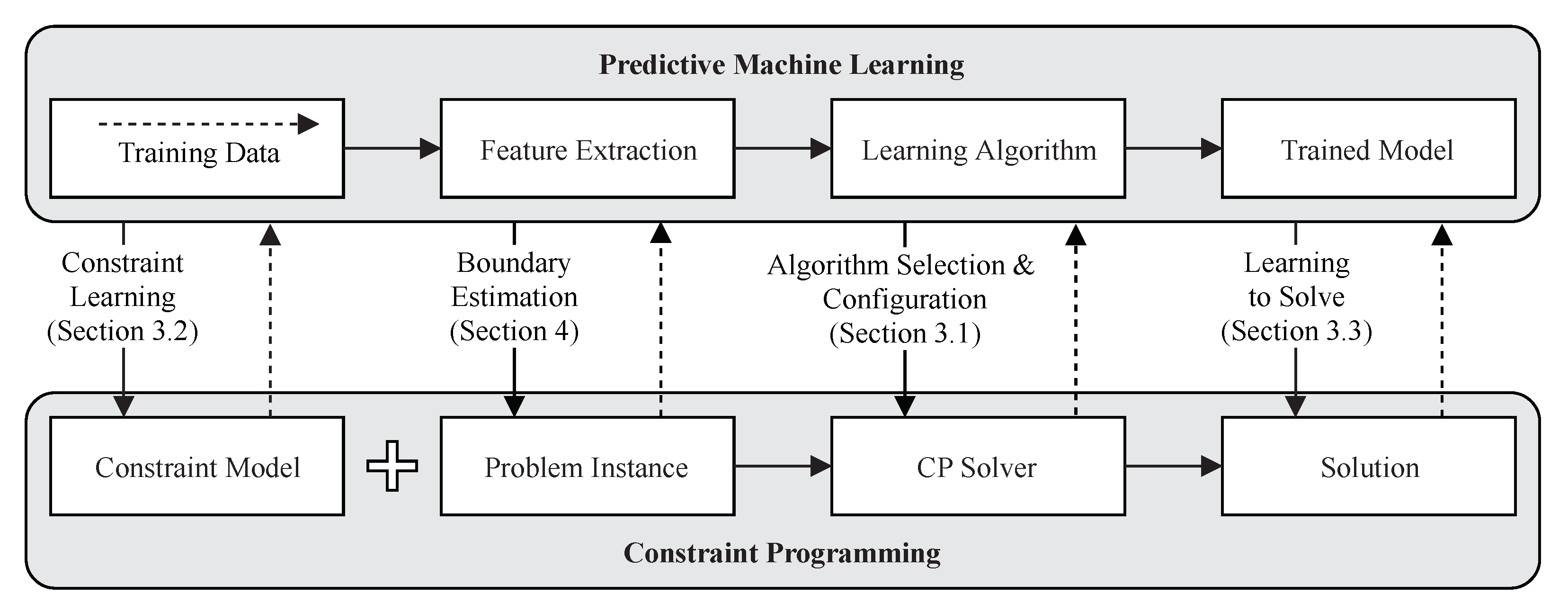
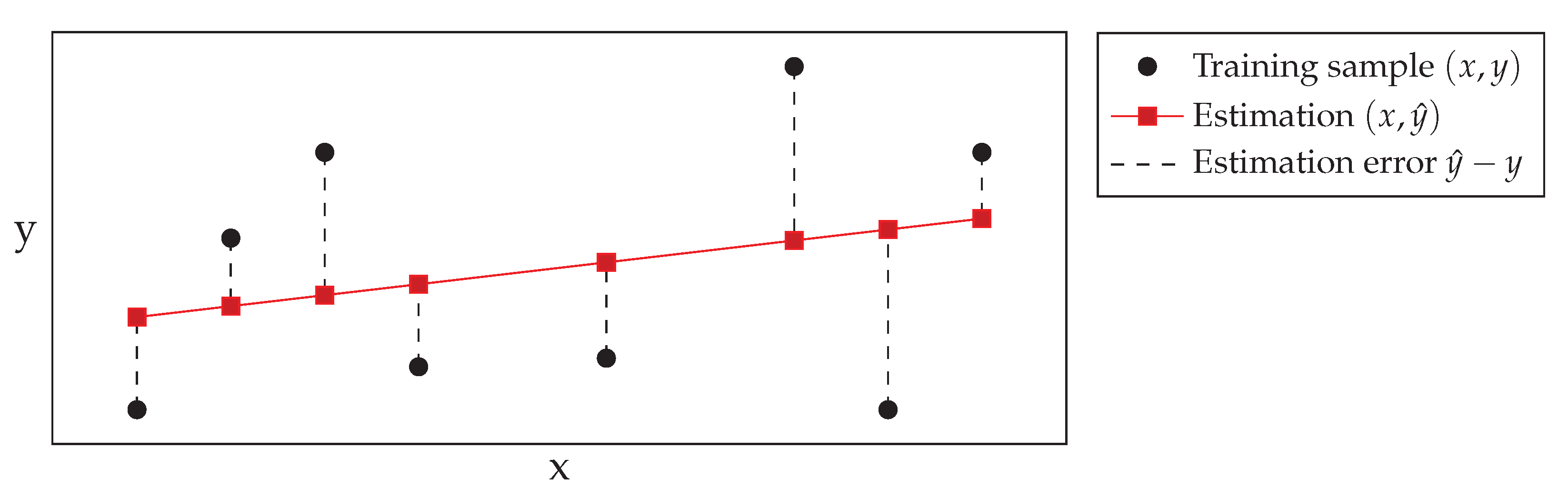
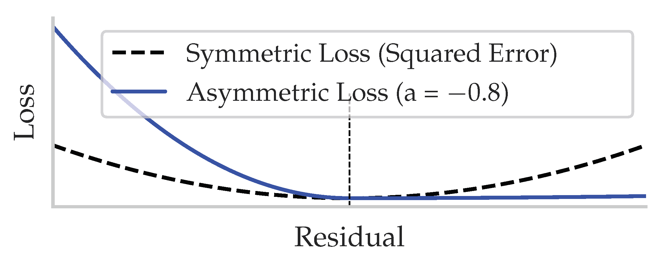
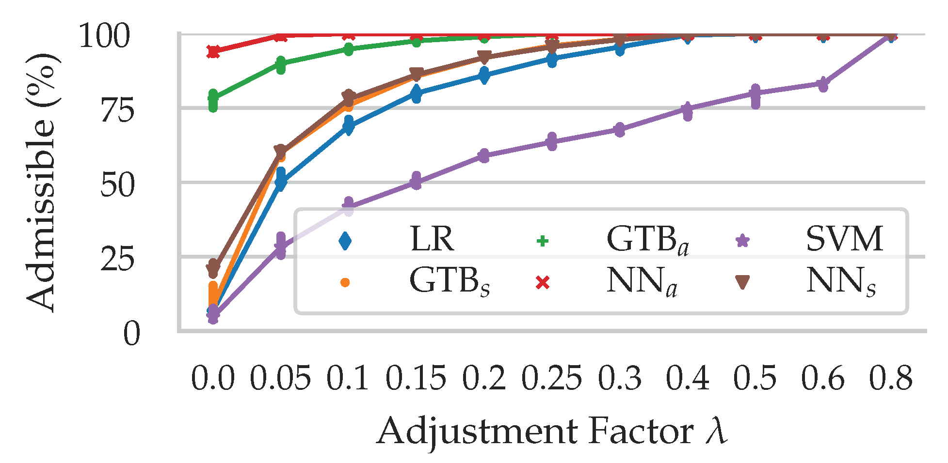
Table 1.
Examples for static COP features from the feature extractor mzn2feat [34], which analyses COPs formulated in the MiniZinc constraint modeling language [35]. The descriptions are quoted from [34]. NV: Number of Variables, NC: Number of Constraints, CV: Variation Coefficient, H: entropy of a set of values.
| Category | Features |
|---|---|
| Variables | The number of variables ; the number of constants; the number of aliases; the ratio ; the ratio ; the number of defined variables (i.e., defined as a function of other variables); the number of introduced variables (i.e., auxiliary variables introduced during the FlatZinc conversion); sum, min, max, avg, CV, and H of the: variables’ domain size, variables’ degree, domain-size-to-degree ratio |
| Domains | The number of: Boolean variables and the ratio ; float variables and the ratio ; integer variables and the ratio ; set variables and the ratio ; array constraints and the ratio ; Boolean constraints and the ratio ; int constraints and the ratio ; float constraints and the ratio ; set constraints and the ratio ; |
| Constraints | The total number of constraints , the ratio , the number of constraints with FlatZinc annotations; the logarithm of the product of the: constraints’ domain (product of the domain size of each variable in that constraint) and constraints’ degree; sum, min, max, avg, CV, and H of the: constraints’ domain, constraints’ degree, domain-to-degree ratio |
| Global Constraints | The total number of global constraints, the ratio and the number of global constraints for each of the 27 equivalence classes in which we have grouped the 47 global constraints |
| Graphs | From the Constraint Graph and the Variable Graph , we compute the min, max, avg, CV, and H of the: nodes’ degree, nodes’ clustering coefficient, nodes’ degree, nodes’ diameter |
| Solving | The number of labeled variables (i.e., the variables to be assigned); the solve goal; the number of search annotations; the number of variable choice heuristics; the number of value choice heuristics |
| Objective | The domain , the degree , the ratios and of the variable v that has to be optimized; the degree of v in the variable graph, its diameter , , . Moreover, named and , the mean and the standard deviation of the variables domain size, and and , the mean and the standard deviation of the variables degree, we compute , , , and |
Table 2.
Overview of the benchmark problems. All considered problems are minimization problems with a large variety in the number of available training instances.
Table 2.
Overview of the benchmark problems. All considered problems are minimization problems with a large variety in the number of available training instances.
| Problem | Objective | Search | Instances |
|---|---|---|---|
| MRCPSP | Max-Max | Model-Specific | 11,182 |
| RCPSP | Leq-Max | Model-Specific | 2904 |
| Bin Packing | Sum | Solver-Default | 500 |
| Cutting Stock | Sum | Solver-Default | 121 |
| Jobshop | Leq-Max | Solver-Default | 74 |
| VRP | Sum | Model-Specific | 74 |
| Open Stacks | Max-Max | Model-Specific | 50 |
Table 3.
Reduction in the objective domain through estimated boundaries (in %). Gap: domain size between the cutting boundary and the optimum (). Size: ratio between the new and initial domain size (). Cells show the median and the Median Absolute Deviation (MAD): no superscript indicate .
Table 3.
Reduction in the objective domain through estimated boundaries (in %). Gap: domain size between the cutting boundary and the optimum (). Size: ratio between the new and initial domain size (). Cells show the median and the Median Absolute Deviation (MAD): no superscript indicate .
| GTB | GTB | LR | NN | NN | SVM | |||||||
|---|---|---|---|---|---|---|---|---|---|---|---|---|
| Gap | Size | Gap | Size | Gap | Size | Gap | Size | Gap | Size | Gap | Size | |
| Bin Packing | 68 | 65 | 60 | 58 | 48 | 48 | 78 * | 68 * | 50 | 48 | 15 | 18 |
| Cutting Stock | 64 * | 66 | 58 * | 59 | 48 * | 49 | 41 *** | 71 + | 48 * | 49 | 29 * | 17 |
| Jobshop | 69 | 69 | 60 | 60 | 50 | 50 | 87 | 81 | 50 | 48 | 19 | 20 |
| MRCPSP | 64 | 61 | 60 | 59 | 49 | 49 | 80 | 76 | 49 | 49 | 13 | 19 |
| Open Stacks | 64 * | 60 + | 59 * | 53 | 43 ** | 43 | 56 ** | 33 * | 47 * | 42 + | 15 + | 15 |
| RCPSP | 65 | 64 | 60 | 60 | 50 | 50 | 80 + | 76 + | 50 | 50 | 13 | 20 |
| VRP | 70 | 70 | 60 | 60 | 50 | 50 | 89 | 88 | 50 | 50 | 0 | 0 |
Table 4.
Effect of boundaries on solver performance (in %). Fixed: upper boundary set to middle between the optimum and first found solution of the unbounded run. Upper: upper boundary set to the estimated boundary. Both: upper and lower boundary set to the estimated boundaries. Results are averaged over 30 instances; lower values are better.
| Equiv. Solution Time | Quality of First | Time to Completion | |||||||
|---|---|---|---|---|---|---|---|---|---|
| Fixed | Upper | Both | Fixed | Upper | Both | Fixed | Upper | Both | |
| Bin Packing | −9.4 | 36.1 | 13.0 | −37.9 | −57.7 | −57.7 | 36.1 | 2140.7 | 2364.5 |
| Jobshop | −96.5 | −96.4 | −96.6 | −38.1 | −60.0 | −60.0 | −27.6 | −53.6 | −42.5 |
| MRCPSP | 0.0 | 0.0 | 0.0 | −10.8 | −0.4 | 0.0 | 1.2 | 0.3 | −3.4 |
| Open Stacks | −1.3 | −1.3 | −0.9 | −24.0 | −13.2 | −13.2 | 2.0 | −0.4 | 2.9 |
| RCPSP | −3.2 | 197.4 | 25.3 | −3.3 | 0.0 | 0.0 | −4.2 | 0.0 | −4.2 |
| VRP | 0.4 | 0.0 | 0.0 | −23.5 | 0.0 | 0.0 | 2.0 | 7.0 | 7.0 |
| (a) Chuffed | |||||||||
| Bin Packing | 53.5 | 0.3 | −0.6 | −4.7 | 0.0 | 0.0 | −10.3 | −4.0 | −13.0 |
| Cutting Stock | 5627.0 | 7.3 | −29.5 | −8.5 | −5.5 | −2.6 | −− | −− | −− |
| Jobshop | 189.3 | −6.4 | 37.4 | −10.9 | 6.1 | 6.1 | 0.0 | 0.0 | 0.0 |
| MRCPSP | 0.0 | 0.0 | 23.6 | −10.8 | −0.4 | −0.2 | 1.3 | 0.0 | 4.0 |
| Open Stacks | 0.0 | −1.5 | 0.0 | −24.0 | −12.8 | −12.8 | 8.9 | 6.4 | 6.8 |
| RCPSP | −17.2 | 56.8 | −14.4 | −2.8 | 0.0 | 0.0 | −11.8 | 12.0 | −9.4 |
| VRP | 0.0 | 0.0 | 0.0 | −21.0 | 0.0 | 0.0 | −19.0 | −18.0 | −8.0 |
| (b) Gecode | |||||||||
| Bin Packing | −22.7 | 35.0 | 39.2 | −37.4 | −57.0 | −57.2 | 104.4 | 170.0 | 172.4 |
| Jobshop | 1.1 | 0.0 | 0.0 | −16.5 | −0.8 | −0.8 | 0.0 | 0.0 | 0.0 |
| MRCPSP | −3.2 | −3.0 | 45.3 | −10.8 | −0.4 | 0.0 | −2.4 | −2.1 | 1.2 |
| Open Stacks | −5.0 | −2.6 | −3.1 | −24.0 | −13.2 | −13.2 | 6.3 | −1.2 | 2.3 |
| RCPSP | 0.0 | 147.2 | 30.4 | −3.3 | 0.0 | 0.0 | −6.6 | 27.0 | 7.8 |
| VRP | −95.3 | 0.0 | 0.0 | −38.2 | 0.0 | 0.0 | 32.0 | −3.0 | −5.0 |
| (c) OR-Tools | |||||||||
Publisher’s Note: MDPI stays neutral with regard to jurisdictional claims in published maps and institutional affiliations. |
© 2021 by the authors. Licensee MDPI, Basel, Switzerland. This article is an open access article distributed under the terms and conditions of the Creative Commons Attribution (CC BY) license (https://creativecommons.org/licenses/by/4.0/).
Share and Cite
MDPI and ACS Style
Spieker, H.; Gotlieb, A. Predictive Machine Learning of Objective Boundaries for Solving COPs. AI 2021, 2, 527-551. https://doi.org/10.3390/ai2040033
AMA Style
Spieker H, Gotlieb A. Predictive Machine Learning of Objective Boundaries for Solving COPs. AI. 2021; 2(4):527-551. https://doi.org/10.3390/ai2040033
Chicago/Turabian StyleSpieker, Helge, and Arnaud Gotlieb. 2021. "Predictive Machine Learning of Objective Boundaries for Solving COPs" AI 2, no. 4: 527-551. https://doi.org/10.3390/ai2040033