Early Detection of Excess Nitrogen Consumption in Cucumber Plants Using Hyperspectral Imaging Based on Hybrid Neural Networks and the Imperialist Competitive Algorithm

Abstract

To achieve healthy and optimal yields of agricultural products, the principles of nutrition must be observed and appropriate fertilizers must be applied. Nutritional deficiencies or overabundance reduce the quality and yield of the products. Thus, their early detection prevents physiological disorders and associated diseases. Most research efforts have focused on spectroscopy, which extracts only spectral data from a single point of the product. The present study aims to detect early excess nitrogen in cucumber plants by using a new hyperspectral imaging technique based on a hybrid of artificial neural networks and the imperialist competitive algorithm (ANN-ICA), which can provide spectral and spatial information on the leaves at the same time. First, cucumber seeds were planted in 18 pots. The same inputs were applied to all the pots until the plants grew; after that, 30% excess nitrogen was applied to nine pots with irrigation water, while it remained constant in the other nine pots. Each day, six leaves were collected from each pot, and their images were captured using a hyperspectral camera (in the range of 400–1100 nm). The wavelengths of 715, 783 and 821 nm were determined as the most effective for early detection of excess nitrogen using a hybrid of artificial neural networks and the artificial bee colony algorithm (ANN-ABC). The parameter of days of treatment was classified using ANN-ICA. The performance of the classifier was evaluated using different criteria, namely recall, accuracy, specificity, precision and the F-measure. The results indicate that the differences between different days were statistically significant. This means that the hyperspectral imaging technique was able to detect plants with excess nitrogen in the near-infrared range (NIR), with a correct classification rate of 96.11%.

1. Introduction

In recent decades, the demand for higher quality agricultural products has increased. Mechanical, bacterial and contamination damage are factors that may shorten the shelf life of fruits and vegetables and reduce their marketability. Therefore, research is being conducted to inspect these products to ensure their quality and health, using non-destructive techniques such as imaging and spectroscopy. However, traditional spectroscopy only provides spectral information from a given location of the products, determining location-dependent quantities. On the other hand, external features of the agricultural products can be extracted using machine vision systems based on visible imaging [1,2,3,4,5,6,7]. However, these systems are incapable of inspecting samples with the same color, classifying complex targets (such as predicting chemical components) and detecting invisible defects, since they capture images using visible wavelengths in the form of monochrome or color images. By integrating the advantages of spectroscopy and imaging, hyperspectral imaging (HSI) can simultaneously provide spectral and spatial information, which is vital for predicting the quality of agricultural products. This technique uses the properties of reflectance, absorption and transmission of light [8,9,10].

In recent years, HSI has emerged as a powerful tool for determining the internal and external features of different types of objects [11,12]. Many applications have been proposed for detecting contaminants, diseases and defects of biological products, among others; for example, prediction of nutrient deficiencies in citrus [13], prediction of micronutrients in wheat [14], diagnosing phosphorus abnormalities and nitrogen deficiency in rice [15,16,17], determination of chlorophyll content in cucumber [18], estimation of chlorophyll content in tea plants [19], early detection of diseases in meat [20], and poisonous fungi on corn [21] and wheat [22].

Ghosal et al. [23] used a relatively simple convolutional neural network (CNN) for classifying soybean into three classes, viz. nutrition-deficient (potassium and iron), herbicide-damaged and healthy. The correct classification rate was 94%. Shamshiri et al. [24] used support vector machines for detecting nitrogen, potassium and magnesium deficiency in palm oil. Audebert et al. [25] compared the effectiveness of support vector machines and deep learning to predict the nitrogen content of tea plants using 120 hyperspectral images of tea leaves. The performance of the support vector model was better than deep learning. Balasubramaniam and Ananthi [26] used c-means fuzzy clustering to classify various types of crops, including chickpea, sugarcane, corn, cotton, cucumber, banana, rice, corn, wheat, canola, coconut, sugar beet and barley, from the viewpoint of deficiencies in manganese (Mn), molybdenum (Mo), phosphorus (P), zinc (Zn), potassium (K) and boron (Br). The accuracy rate varied from 0.91 to 0.99, depending on the type of product and the nutrient deficiency. Backhaus et al. [27] mentioned that the age of leaves was a major factor in determining nutritional stress using hyperspectral imaging; they reported that the results from young leaves had statistically significant differences compared with other leaves. The growth stage and age of leaves had different effects in the spectral information. In the case of regression techniques, it may be necessary to extract separate models for different plant growth stages. Condori et al. [28] used the CNN model to detect nitrogen deficiency in maize, wherein three growth stages were considered using 384 hyperspectral images. The results showed that the growth stage was an effective factor. Mogollón et al. [29] used a simple Bayes method to classify magnesium (Mg) content in corn. The leaves were sampled at three growth stages. The best classification accuracy, obtained using fractal dimension with focal analysis was 75%.

Observing the principles of nutrition and applying appropriate fertilizer is the key factor for achieving healthy agricultural products. Symptoms of nutritional disorders of cucumber often appear on the leaves. Fertilization should be based on regular analysis of the soil and leaves. Often, farmers do not pay attention to the symptoms of nutrition deficiency on the leaves, although it can reduce the quality and yield of the crops. Reliable diagnosis of the nutritional status of plants is an essential part of farm management, as both excess and deficiencies of nutrients can cause severe damage and reduced yields; therefore, early detection of nutritional problems makes it possible to control biological disorders. Moreover, it reduces environmental impact. Leaf laboratory analysis is an accurate method, but it is destructive and time-consuming [30].

The present study aimed to early detect excess nitrogen consumption in cucumber plants using a hyperspectral imaging technique based on artificial neural networks and the imperialist competitive algorithm (ANN-ICA). The hybrid ANN-ICA approach was applied to find the optimal configuration of the neural network, which is responsible for detecting excess nitrogen in plants. The main innovations of the proposed method are: (1) extraction of images of the leaves at different wavelengths in the range from 400 to 1100 nm to find the most effective hyperspectral images for classification; (2) selection of the key wavelengths using hybrid artificial neural networks and the artificial bee colony algorithm (ANN-ABC) to obtain the most useful spectral information; (3) classification using a hybrid artificial neural network (ANN) with an optimal structure that guarantees the high accuracy of the method; and (4) training the system at different iterations to examine the reliability of the proposed system.

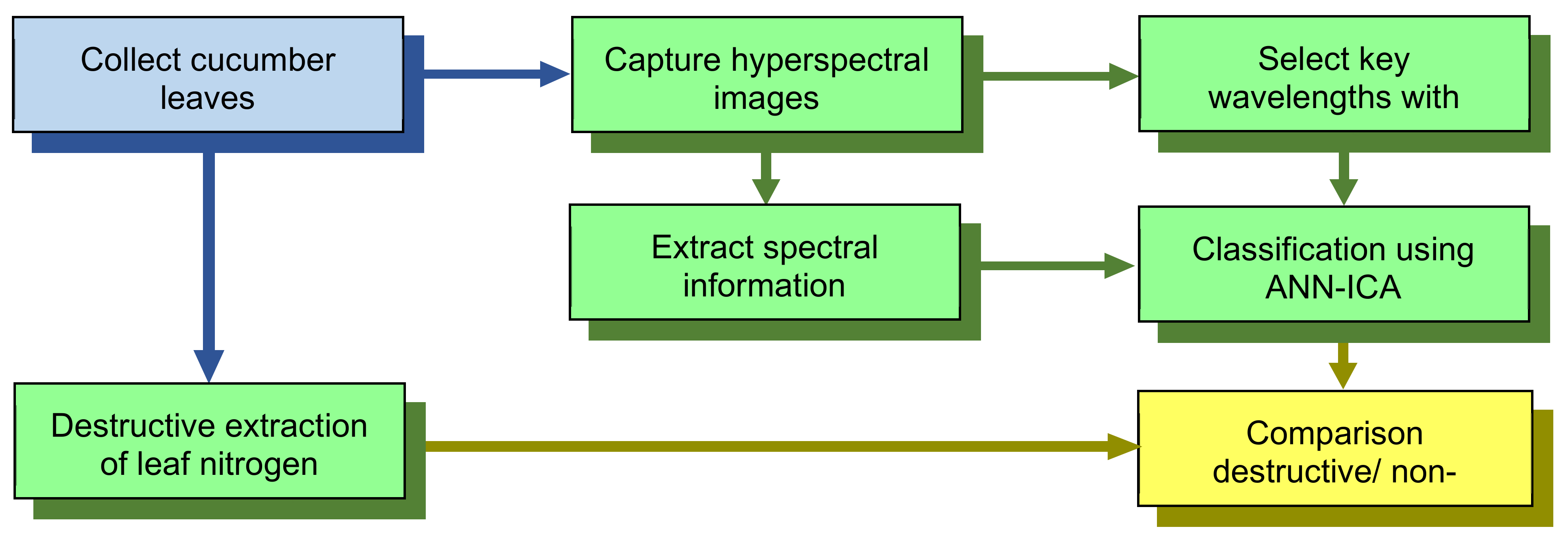
2. Materials and Methods

Figure 1 shows the main steps of the research process carried out in the present study, from the collection of the cucumber leaves used in the experiments to the comparison of the proposed method with a traditional laboratory analysis of the nitrogen content. These steps are described in detail in the following subsections.

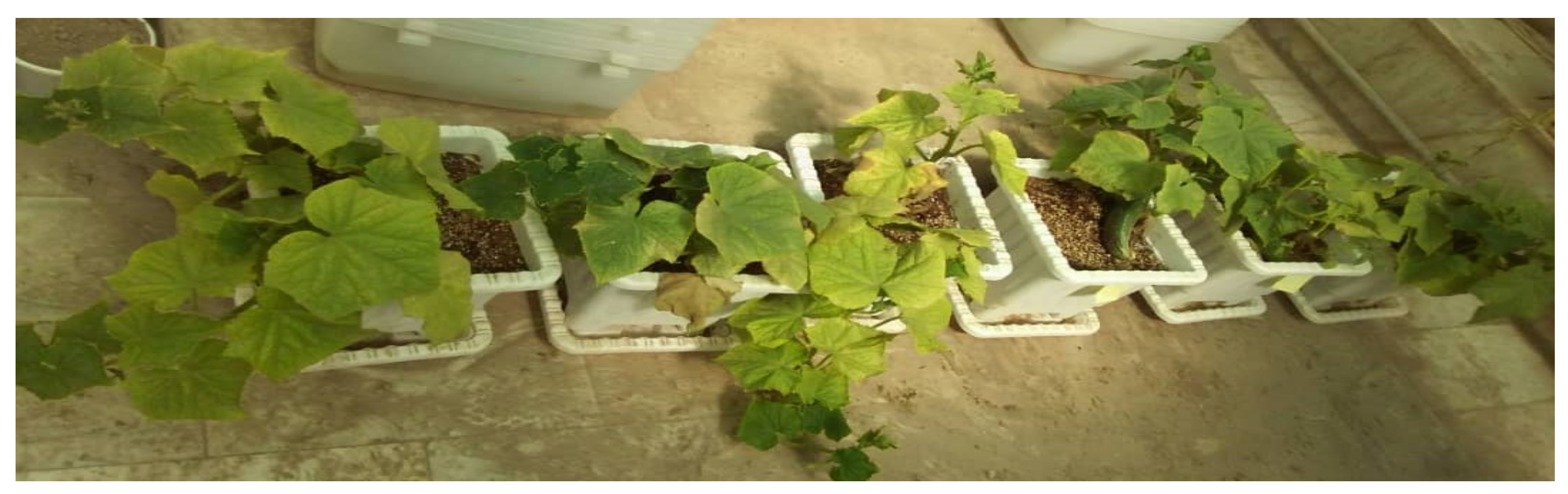
2.1. Data Collection

Initially, 18 pots were prepared and cucumber seeds (Super Arshiya-F1 cultivar) were planted in each pot and kept in the research greenhouse of the University of Mohaghegh Ardabili, Iran, as shown in Figure 2. All the pots consumed the same inputs until the plants grew. After that, 30% excess nitrogen was applied with irrigation water to 9 pots. Next, 6 leaves were picked from each pot every day, and hyperspectral images of these leaves were captured with a hyperspectral camera. The sampling process continued until the leaves turned yellow and the symptoms of fertilizer overapplication were clearly visible. This occurred on the fourth day, so the images go from Day 0 (just before applying excess nitrogen) until Day 3.

The increase of 30% in the application of nitrogen was selected by considering some previous works related to the use of fertilizers. For example, Ma et al. [31] presented a method to detect deficiencies and excess of nitrogen in soybean leaves using RGB color images, with levels of nitrogen of 0%, 50%, 100% and 150%. Yang et al. [32] analyzed the effect of different levels of nitrogen in cucumber yield and fertilization efficiency, with application levels of 250, 300 and 350 kg/hm², i.e., 20% and 40% increases, respectively. Thus, our selection of a 30% increase can be considered as an average value, trying to detect the excess nitrogen in relatively low increments.

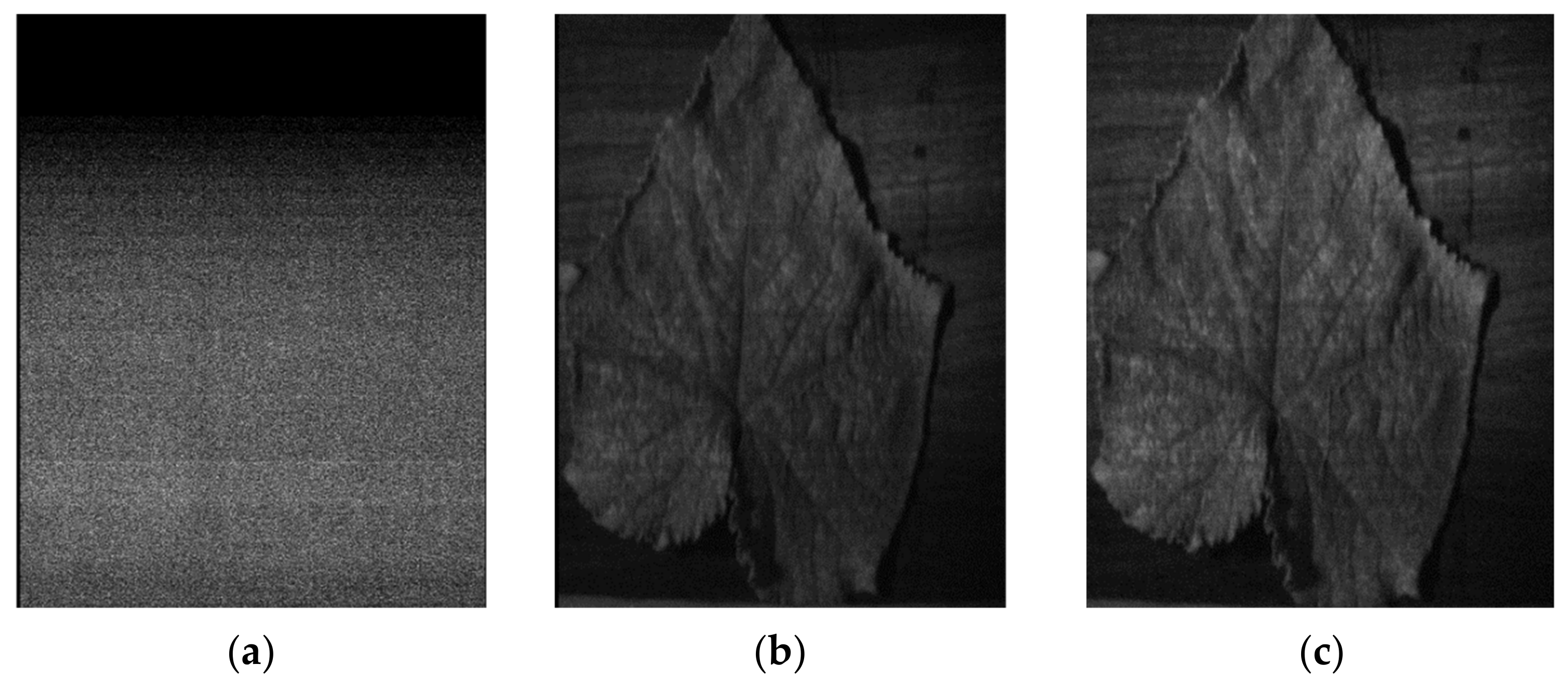
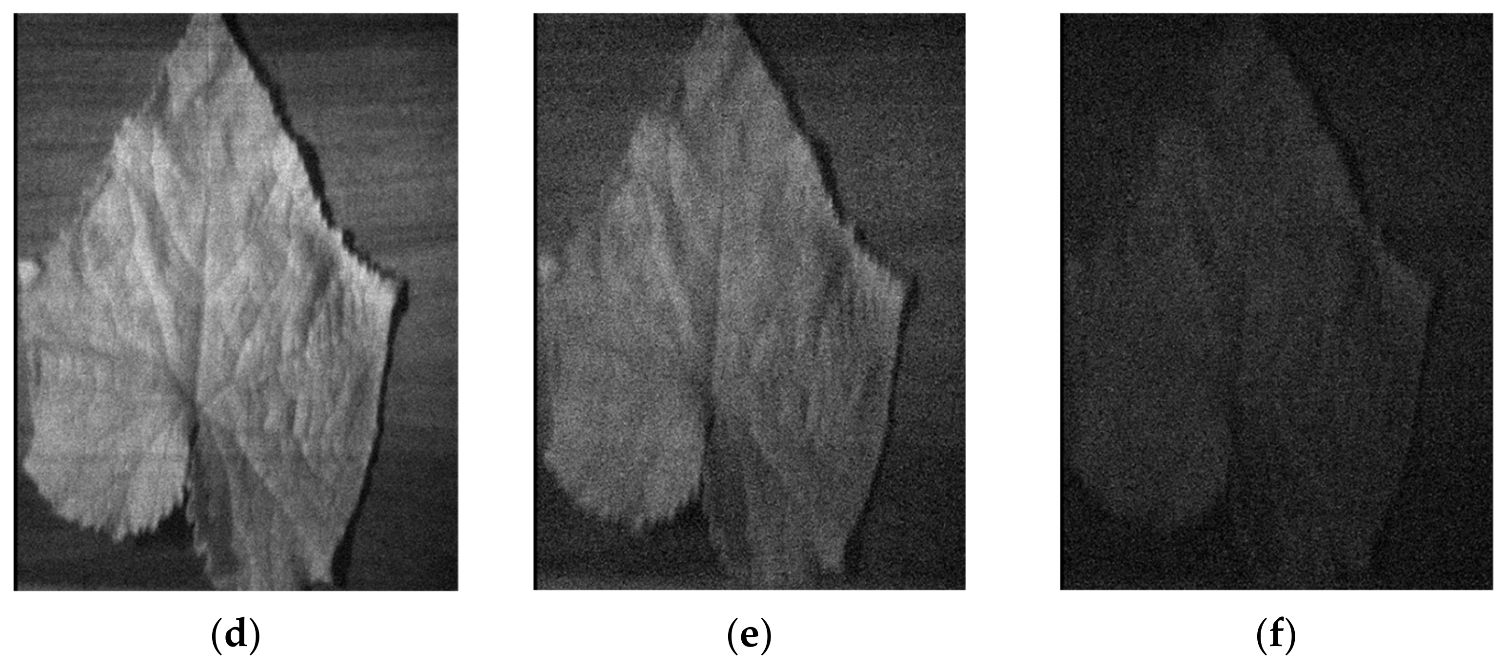
2.2. Capturing Hyperspectral Images and Extracting the Spectral Properties of the Leaves

To extract spectral images from the leaves, a hardware system was configured. The components of this system were: (1) a laptop with Intel Corei5CFI, 330 M at 2.13 GHz, 4 GB of RAM, and Windows 10; (2) a hyperspectral camera (FSR, Fanavaran Physics Noor Co., Tehran, Iran) with a spectral range from 400 to 1100 nm; (3) a light source of tungsten halogen with a power of 10 W (StellarNet, Tampa, FL, USA) and (4) an illumination chamber to prevent ambient light. The hyperspectral camera was located on the left side of the chamber, and the samples were located horizontally in front of the camera at a distance of 1 m. A pair of lamps illuminated the sample from the corners, as depicted in Figure 3.

Figure 4 shows some examples of the hyperspectral images of cucumber leaves in the range of 400–1100 nm. The image resolution is 400 × 640 pixels, with a depth of 8 bits per pixel for each wavelength.

In total, 327 images of wavelengths in the range of 400–1100 nm were captured for each cucumber leaf. As can be seen, at the beginning and the end of this range, the images have poor quality due to noise and lack of illumination. These images were also included in further processing but were automatically removed since they were not effective. Moreover, although the images contain a part of the background, as shown in Figure 4, these background pixels were removed from the analysis.

2.3. Selection of the Key Wavelengths for Early Detection of Excess Nitrogen

After imaging the leaves from pots with normal nitrogen levels and with excess nitrogen, a hybrid approach of artificial neural networks and the artificial bee colony algorithm (ANN-ABC) was used to find the most interesting wavelengths for the subsequent processes. ABC is a heuristic optimization process proposed by Pham et al. [33]. This algorithm is inspired by the behavior of bees in their search for food sources [34]. The steps of the ABC algorithm are as follows:

• First, the initial responses (or candidate sites) are generated and evaluated.
• The better responses are selected and the scout bees are sent to those sites.
• The scout bees return to the hive with a waggle dance (producing a neighboring response).
• All the answers are compared and the best one is selected.
• The position of the best answer is saved.
• If the ideal conditions are not met, return to Step 2.

Following this scheme, in this study, different vectors of wavelengths were sent as the input to an artificial neural network, and the output of the network was the corresponding nitrogen content of the leaf (i.e., the number of days of application of excess nitrogen). For example, consider that the selected vector of wavelengths is (700, 800, 900 nm); this means that the ANN receives tuples of 3 values, corresponding to the light intensities in these spectral frequencies for a given pixel of the images. For each vector of wavelengths, a complete process of training the ANN and testing the trained network on the test set was done. Each vector was recorded together with the answer to this input, which was given by the mean squared error (MSE) produced by the ANN in the classification of the test set. The vector with the least MSE was then selected as the optimal input, and the related wavelengths were selected as the key wavelengths. The structure of the ANN used in this procedure is presented in

Table 1. Structure of hidden layers of the artificial neural network (ANN) used to select the key wavelengths in the artificial neural networks and the artificial bee colony algorithm (ANN-ABC) process.

Property	Value
Number of hidden layers	1
Number of neurons	13
Transfer function	Radial basis
Back-propagation network training function	Levenberg-Marquardt
Back-propagation weight/bias learning function	Hebb weight learning rule

.

2.4. Pre-Processing of the Spectral Data

As depicted in Figure 4, the original data may be affected by noise due to the light source, the effect of the ambient light, the camera and so on. Therefore, the data must be pre-processed [35]. In this study, reflective spectral data were first converted to absorption using the following equation:

Absorption spectra = log(1/Reflectance spectra)

(1)

The light scattering was then corrected by a standard normal distribution (SNV) with wavelet detrending. Finally, the smoothing operation was performed with the Savitzki-Golay filter using ParLeS software, version 3.1 [36]. ParLeS is a specialized chemometrics software package that is used for multivariate modeling and forecasting, as shown in Figure 5.

2.5. Destructive Extraction of Nitrogen in the Laboratory

The process for extracting and measuring nitrogen in the leaves was a destructive laboratory procedure, using the classical Kjeldahl method [37]. Figure 6 depicts the equipment used in this process. The method consists of five steps:

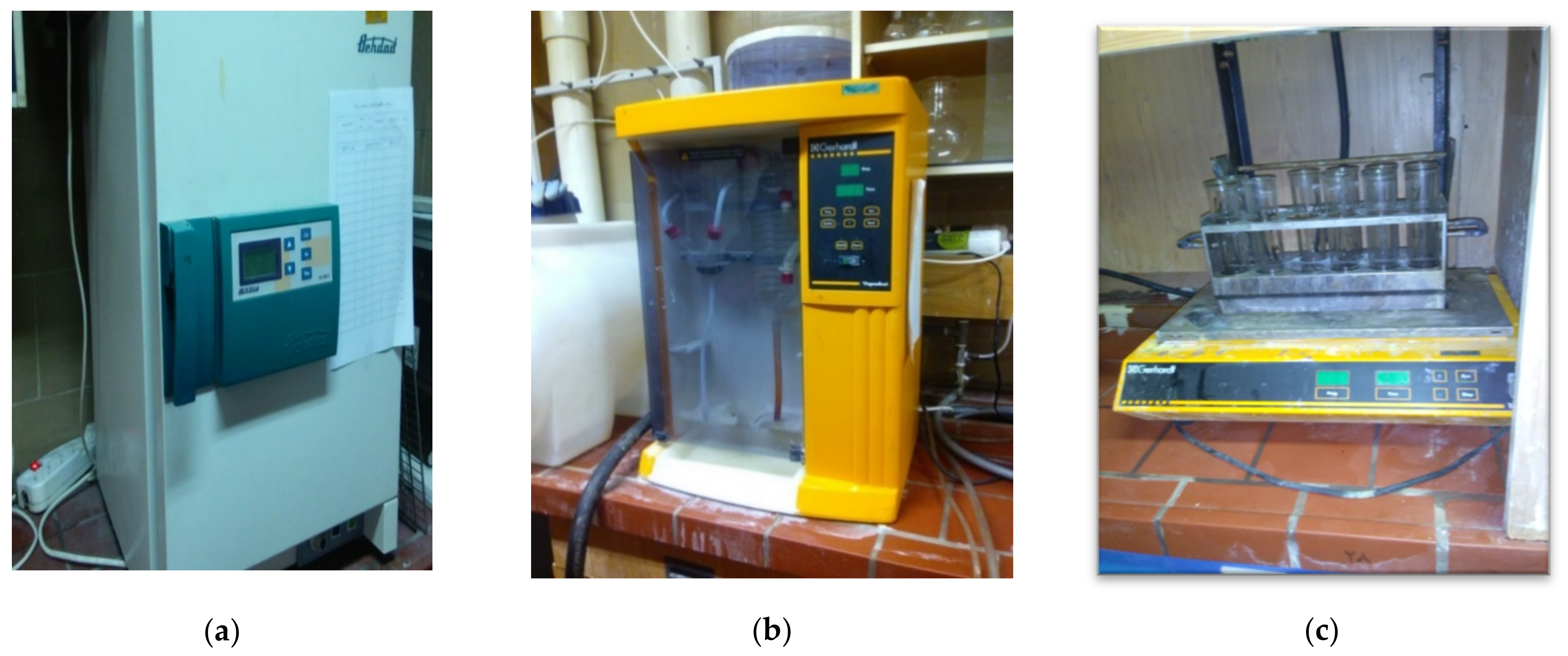
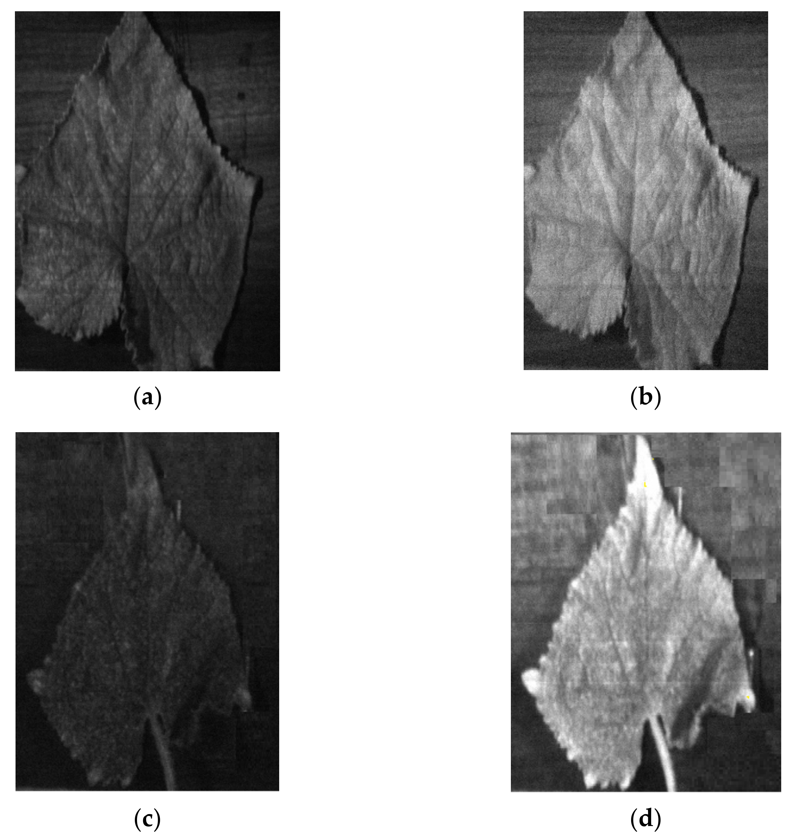
• Powdering. The samples (leaves) must first be powdered. For this purpose, an oven (model BC OVEN 70, Behdad Co., Tehran, Iran) was used. It is made of stainless steel, resistant to high heat and has an electrical protection system, as shown in Figure 6a.
• Kjeldahl device. In order to measure the total leaf nitrogen, a Kjeldahl device (model VAP20, Gerhardt GmbH & Co., Königswinter, Germany) was used, as shown in Figure 6b. The Kjeldahl method proceeds with the steps of digestion, distillation and titration to determine total nitrogen. First, the sample is digested with sulfuric acid; next, the nitrogen of the sample is converted to ammonium sulfate. The nitrogen of ammonium sulfate is then released in the form of ammonia and converted to ammonium borate with boric acid, titrated using normal sulfuric acid 1% and, finally, the total nitrogen content of the sample is obtained by calculating the consumed acid.
• Digestion. The first step in the standard procedure to determine total nitrogen of leaf is digestion. In this study, a digester of model VAP20 (Gerhardt GmbH & Co., Königswinter, Germany) was used, as can be seen in Figure 6c. It has 12 digestion stands. The main characteristics of this device include safety, processing of fatty and inhomogeneous samples, the possibility of digestion of samples with very low volume, an automatic digestion system with temperature control, and an automatic digestion system with time control.
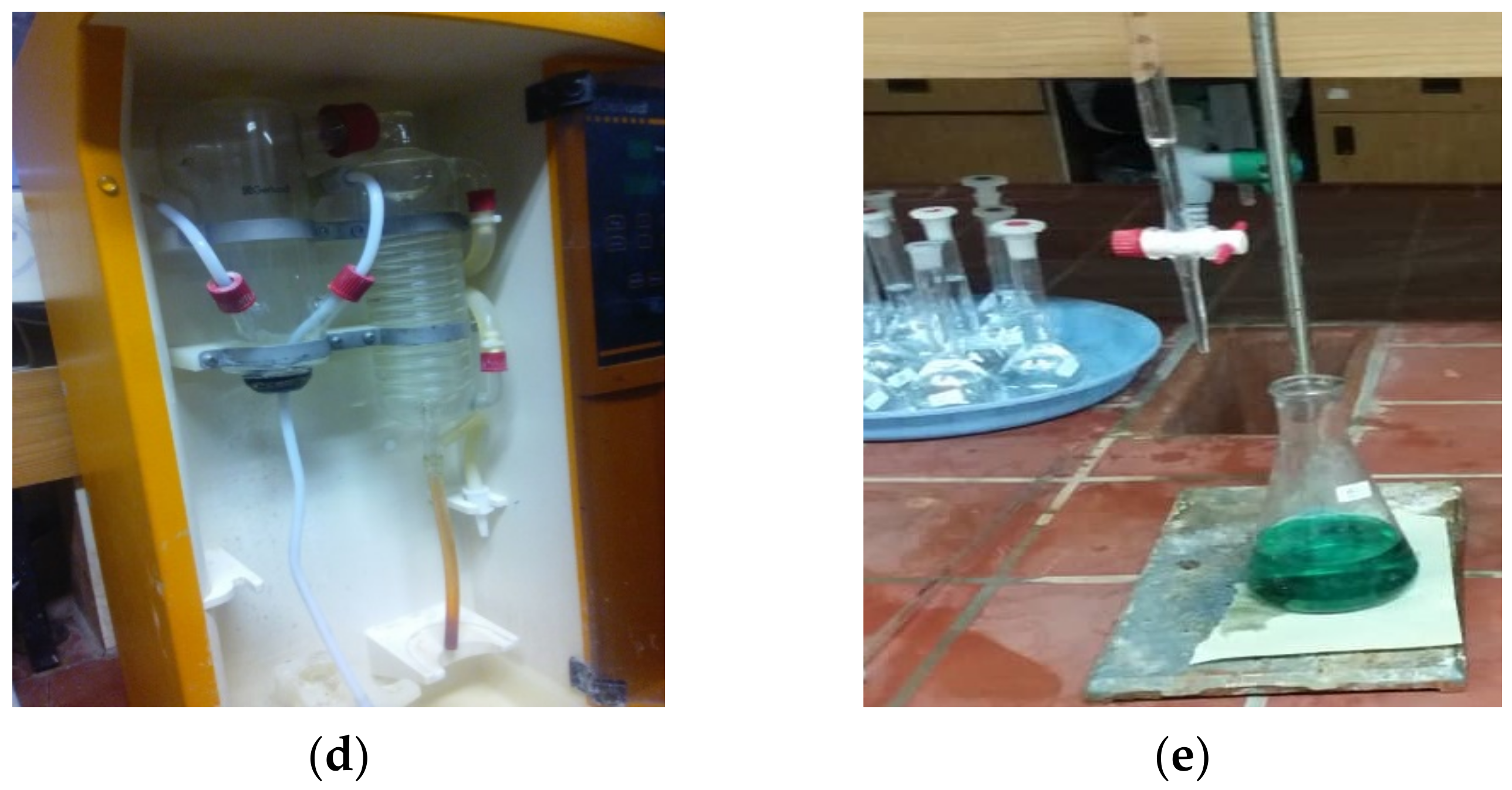
• Distillation. After the digestion step, a refrigerant was used to distill the sample. Distillation was performed in the shortest possible time by adding distilled water and NaOH at 32%. The heat required for distillation was supplied by constant-pressure steam, presented in Figure 6d.
• Titration. The last step is titration, which was carried out with a burette made of glass with a stopper and a valve at the tip to control the flow of the chemical solution.

After the titration step, the total nitrogen was obtained by calculating the acid consumption as:

Total N = (Vs-Vb)/md × N_H2SO4 × 0.014_meqN × 100

(2)

where Vs is the consumed volume of the sample, Vb is the consumed volume of the control treatment, md is the dry weight of the sample and N_H2SO4 is the normality of sulfuric acid with 0.014 mEq.

Figure 6. Laboratory equipment used for measuring the total nitrogen content of the leaves: (a) oven; (b) Kjeldahl device; (c) digestion; (d) distillation; (e) titration.

Figure 6. Laboratory equipment used for measuring the total nitrogen content of the leaves: (a) oven; (b) Kjeldahl device; (c) digestion; (d) distillation; (e) titration.

2.6. Classification of the Days of Application of Nitrogen to the Pots Using ANN-ICA

The objective of the present study was to detect excess nitrogen consumption using hyperspectral images in the key wavelengths selected. For this purpose, the images of the leaves were classified using an ANN, whose output was the number of days of application of excess nitrogen, as previously described. In this way, the system was able to predict overapplication of nitrogen in the early stages. Various parameters had to be set in the configuration of the ANN, which greatly affected the accuracy achieved in the classification. These included the number of hidden layers, the number of neurons, transfer functions, the back-propagation network training function, and back-propagation weight/bias learning function. In our case, the imperialist competitive algorithm (ICA) algorithm was used to optimally adjust the parameters of the ANN.

ICA is a metaheuristic algorithm based on cultural, social and political evolution. In this algorithm, all countries are looking for the general optimal point to solve an optimization problem [38,39]. As in the hybrid ANN-ABC approach, ICA controls the execution of the ANN under different configurations, combining the aforementioned parameters of the ANN and selecting the optimal configuration of the network. Specifically, the number of hidden layers can be between 1 and 3. The number of neurons in each hidden layer can be between 0 (no hidden layer) and 25. The transfer function for each layer was selected from a set of 8 transfer functions available in the neural network toolkit of MATLAB (MathWorks, Natick, MA, USA) such as tangential sigmoid, radial basis and softmax. The back-propagation training function was selected from a set of 6 functions, and the back-propagation weight/bias learning function was selected from a set of 15 different functions available in the same toolkit.

During the ANN-ICA process, the method considers a vector with a selection of the parameters, representing a specific configuration of the ANN. For example, the vector x = [13, logsig, traingdx, learnos] indicates that the ANN has 1 hidden layer with 13 neurons, a log-sigmoid transfer function, gradient descent with momentum back-propagation, and the Outstar weight/bias learning function, respectively. The MSE of each vector obtained in the training/test process of the ANN was measured and the vectors with the lowest MSE were selected as the optimal configuration of the network.

Table 2. Structure of hidden layers obtained by the artificial neural networks and the imperialist competitive algorithm (ANN-ICA) for the classification. Transfer functions: poslin: positive linear; satlins: symmetric saturating linear; tribas: triangular basis.

Property	Value
Number of hidden layers	3
Number of neurons per layer	1st: 12; 2nd: 9; 3rd: 21
Transfer functions	1st: poslin; 2nd: satlins; 3rd: tribas
Back-propagation network training function	Batch training
Back-propagation weight/bias learning function	Instar weight learning function

shows this selection of the parameters obtained by ANN-ICA.

After selecting the optimal structure of the ANN, 200 iterations were executed to evaluate the validity of the classifier. In all the iterations, 60% of the total data were randomly selected for training, 10% for validation and the remaining 30% for testing.

2.7. Evaluation of the Performance of the ANN-ICA Classifier

Different criteria are commonly applied to evaluate the performance of a classifier. Two groups can be distinguished. The first category includes the performance parameters extracted from the confusion matrix, i.e., recall, accuracy, specificity, precision and the F-measure. The second category is given by the graphical criteria associated with the receiver operating characteristic curve (ROC) and the area under the ROC curve (AUC) [2].

Table 3. Performance parameters of a classifier associated with the confusion matrix. TP: true positives; TN: true negatives; FN: false negatives; FP: false positives.

Name	Equation	Description
Recall	$\frac{TP}{TP+FN}\times 100$	Percentage of positive samples that have been correctly identified
Precision	$\frac{TP}{TP+FP}\times 100$	Percentage of positive outputs that have been correctly classified
Accuracy	$\frac{TP+TN}{TP+FN+FP+TN}\times 100$	Percentage of total correct classifications
Specificity	$\frac{TN}{TN+FP}\times 100$	Percentage of negative samples that have been correctly identified
F-measure	$\frac{2\times Recall\times Precision}{Recall+Precision}$	Harmonic weighted average of recall and precision

contains the definitions of the parameters in the first group.

3. Results and Discussion

3.1. Key Wavelengths for Classifying Leaves from Different Days

The key wavelengths for early and non-destructive detection of leaves with excess nitrogen were obtained using the ANN-ABC approach described in Section 2.3. The selected wavelengths were 715, 783 and 821 nm. Figure 7 presents some samples of the hyperspectral images of the selected wavelengths for different days.

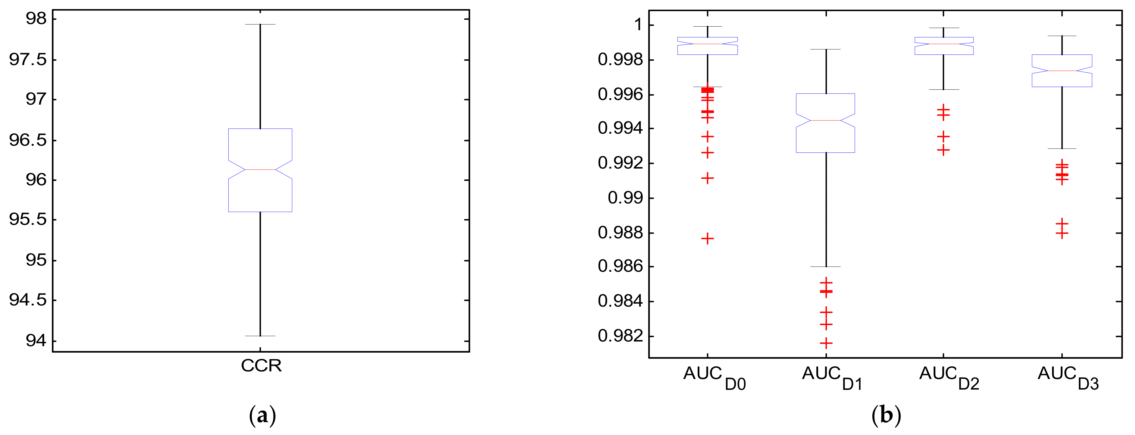
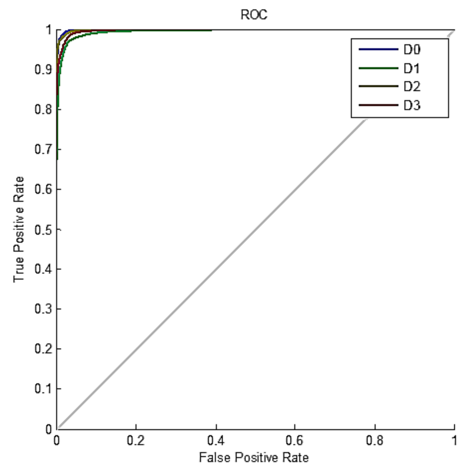
3.2. Performance of ANN-ICA for the Classification of Leaves with Excess Nitrogen

As described in Section 2.6, the hybrid ANN-ICA method was used to predict the number of days when the leaves began to receive excess nitrogen using the images of the selected wavelengths.

Table 4. Evaluation of the performance of the ANN-ICA classifier using the confusion matrix at 200 repetitions. D0: the day before applying excess nitrogen; D1, D2 and D3: one, two and three days after applying excess nitrogen, respectively.

Predicted/ Real Class	D0	D1	D2	D3	Total	Class Error Rate (%)	CCR (%)
D0	44,872	899	49	0	45,820	2.06	96.11
D1	1079	40,914	151	957	43,101	5.07
D2	1	617	29,581	416	30,615	3.37
D3	0	1008	847	33,609	35,464	5.23

presents the performance of the classifier using the confusion matrix, the accuracy or correct classification rate (CCR) and the error rate for the 200 iterations of the training/test process. This makes an equivalent of 155,000 test samples. Only 6024 of these samples were incorrectly classified in the wrong class. This number of misclassifications resulted in a total accuracy of 96.11%.

Table 5. Evaluation of the performance of the ANN-ICA classifier at 200 repetitions, using the criteria derived from the confusion matrix.

Class	Recall (%)	Accuracy (%)	Specificity (%)	Precision (%)	F-Measure (%)
D0	97.64	98.65	99.09	97.93	97.79
D1	94.18	96.93	98.01	94.92	94.55
D2	96.58	98.62	99.14	96.62	96.60
D3	96.07	98.87	98.41	94.76	95.41

evaluates the same results using the five performance criteria, namely recall, accuracy, specificity, precision and F-measure. A recall of 100% means that none of the samples was incorrectly classified in the given class; thus, the low recall obtained for D1 (94.18%) means that most of the samples were incorrectly classified in class D1. The reason is that in the early hours, it is more difficult to identify excess nitrogen than in the following days. According to the table, it is obvious that more samples were classified correctly in class D3 than in other classes, since the accuracy of class D3 was the highest (98.87%). In fact, on the third day, the leaves reacted clearly to the excess nitrogen and it was easy to detect them visually. The value of specificity was 99.14% for class D2, which was higher than the others. It means that class D2 had the least error. The accuracy was 94.76% for class D3, which was the lowest value among all classes, indicating that many samples were incorrectly classified in other classes. Finally, since the F-measure is the weighted harmonic mean of recall and accuracy, it can be understood that the value for class D0 was higher than the others.

Figure 8 represents the performance of the classifier using box plots of CCR and AUC for the 200 repetitions of the process. According to the results in Figure 8b, the box plot diagrams of AUCs are compact for all classes, indicating the high performance and stability of this classifier. It is also evident from the box plots that although the excess nitrogen could be detected on the first day after applying it (D1), from the second day onwards (D2 and D3), the AUC charts increased. This indicates that the detection algorithm had higher performance on D2 and D3 than on D1, as expected. However, contrary to expectations, the AUC of D2 was higher than that of D3. This could be due to newly sprouted leaves on the third day, which, compared with the older leaves, produced errors. However, these errors were not large enough to cause statistically significant differences.

Figure 9 shows the ROC curves of the classifier averaged for the 200 repetitions. These curves are independent of the number of samples in each class and only examine the performance of the classifiers based on the ratio of incorrectly classified samples; the lower the curves, the lower the performance of a classifier. According to Figure 9, the ROC curves of all the classes are very close to the ideal curve, indicating the very high performance of the proposed algorithm.

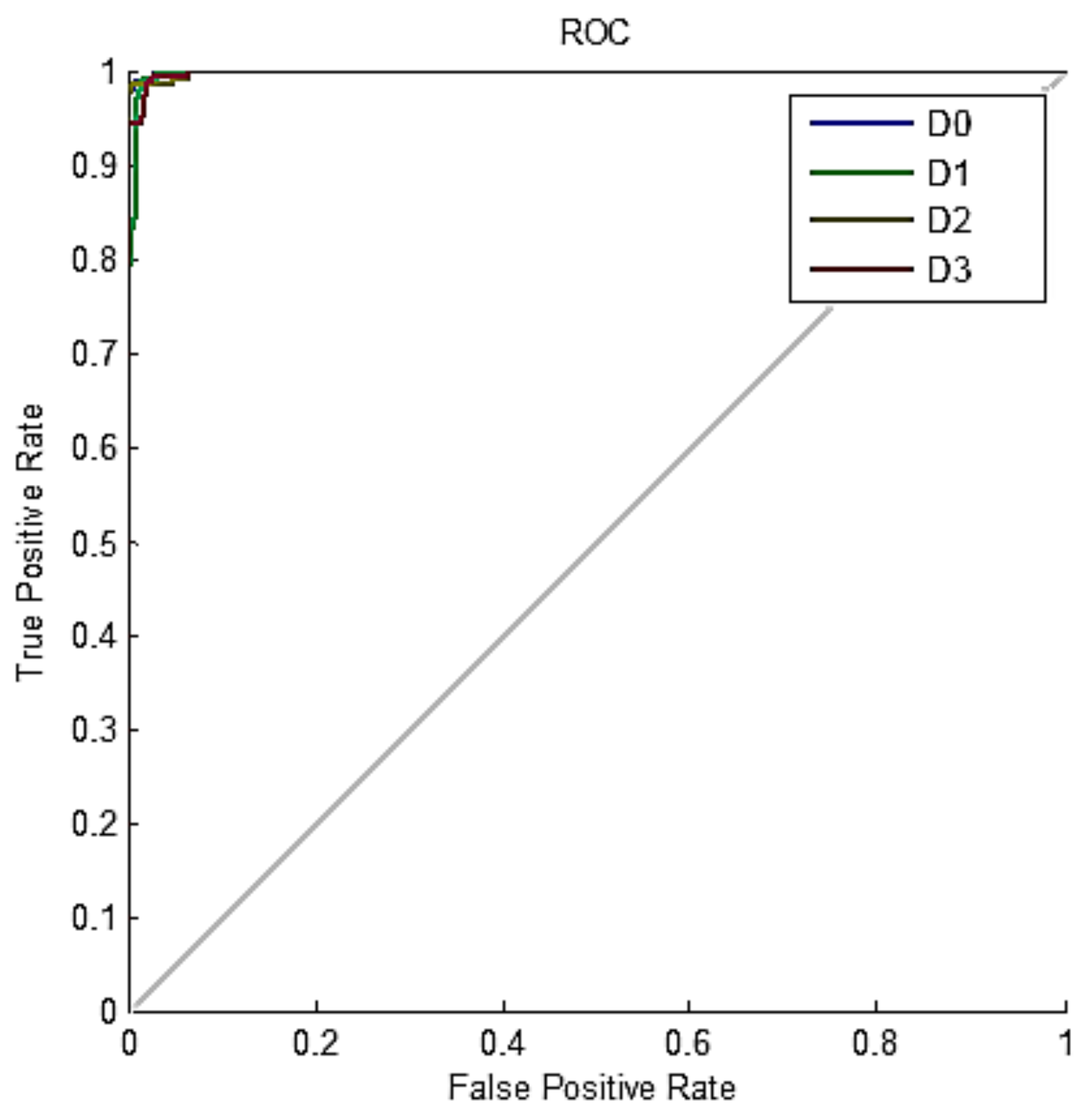
3.3. Performance of the Classifier in the Best Training Case

From the 200 repetitions of the training/test process, we considered it interesting to extract the results of the best case. The performance measures for this specific case are presented in

Table 6. Evaluation of the performance of the ANN-ICA classifier for the best training case.

Predicted/Real Class	D0	D1	D2	D3	Total	Class Error Rate (%)	CCR (%)
D0	237	4	0	0	241	1.65	97.93
D1	1	219	0	4	224	2.23
D2	0	2	142	0	144	1.38
D3	0	2	3	161	166	3.01

and

Table 7. Evaluation of the performance of the ANN-ICA classifier using the criteria derived from the confusion matrix, for the best training case.

Class	Recall (%)	Accuracy (%)	Specificity (%)	Precision (%)	F-Measure (%)
D0	99.57	99.34	99.23	98.34	98.95
D1	96.47	98.31	99.08	97.76	97.11
D2	97.93	99.34	99.67	98.61	98.26
D3	97.57	98.82	99.17	96.98	97.28

and in Figure 10.

Table 8. Performance of the ANN-ICA classifier for early detection of excess nitrogen using spectral data, comparing the mean and standard deviation (SD) of the 200 repetitions, and the best case.

Execution	CCR (%)	AUCD0	AUCD1	AUCD2	AUCD3
Mean	96.11	0.9985	0.9938	0.9986	0.9969
SD	0.739	0.00143	0.00314	0.00099	0.00195
Best	97.93	0.9996	0.9978	0.9991	0.9986

compares the performance of the ANN-ICA classifier using the mean and standard deviation of the CCR and AUC for the 200 repetitions and the best training case. As shown, the CCR and AUCs in the best training case indicate that the proposed algorithm was able to detect excess nitrogen early.

3.4. Statistical Analysis of the Key Wavelengths Using ANOVA and Tukey’s Test

To ensure a reliable classification of the proposed algorithm, a statistical analysis was performed on the effective spectrum data using ANOVA and the Tukey test. The null hypothesis (H₀) was that the spectral images of the key wavelengths were equal for all the days of treatment, and the alternative hypothesis (H_a) was that they were different. While the ANOVA tests only inform whether there are some differences in the means, the Tukey test analyzes which means are different from the others. For conciseness, the results of these tests are shown in

Table A1. Statistical analysis of ANOVA for the key wavelength of 715 nm for the four excess nitrogen treatments.

	Sum of Squares	Degrees of Freedom	Mean Square	F	Significance
Between groups	96.256	3	32.085
Within groups	39.493	2581	0.015	2097	0.000
Total	135.749	2584

,

Table A2. Statistical Tukey’s honestly significant difference (HSD) test for the key wavelength of 715 nm for the four excess nitrogen treatments: D0, D1, D2 and D3.

I Class	J Class	Mean Difference (I–J)	Standard Error	Significance
D0	D1	−0.26439385 *	0.00642292	0.000
	D2	0.05836787 *	0.00707141	0.000
	D3	−0.43466605 *	0.00677766	0.000
D1	D0	0.26439385 *	0.00642292	0.000
	D2	0.32276172 *	0.00715925	0.000
	D3	−0.17027220 *	0.00686926	0.000
D2	D0	−0.05836787 *	0.00707141	0.000
	D1	−0.32276172 *	0.00715925	0.000
	D3	−0.49303392 *	0.00747914	0.000
D3	D0	0.43466605 *	0.00677766	0.000
	D1	0.17027220 *	0.00686926	0.000
	D2	0.49303392 *	0.00747914	0.000

* The mean difference is statistically significant at the 0.05 level.

,

Table A3. Statistical analysis of ANOVA for the key wavelength of 783 nm for the four excess nitrogen treatments.

	Sum of Squares	Degrees of Freedom	Mean Square	F	Significance
Between groups	87.467	3	29.156
Within groups	22.280	2581	0.009	3378	0.000
Total	109.747	2584

,

Table A4. Statistical Tukey’s HSD test for the key wavelength of 783 nm for the four excess nitrogen treatments: D0, D1, D2 and D3.

I Class	J Class	Mean Difference (I–J)	Standard Error	Significance
D0	D1	−0.33859174 *	0.00482421	0.000
	D2	−0.27702890 *	0.00531128	0.000
	D3	−0.48981082 *	0.00509064	0.000
D1	D0	0.33859174 *	0.00482421	0.000
	D2	0.06156284 *	0.00537726	0.000
	D3	−0.15121908 *	0.00515945	0.000
D2	D0	0.27702890 *	0.00531128	0.000
	D1	−0.06156284 *	0.00537726	0.000
	D3	−0.21278192 *	0.00561752	0.000
D3	D0	0.48981082 *	0.00509064	0.000
	D1	0.15121908 *	0.00515945	0.000
	D2	0.21278192 *	0.00561752	0.000

* The mean difference is statistically significant at the 0.05 level.

,

Table A5. Statistical analysis of ANOVA for the key wavelength of 823 nm for the four excess nitrogen treatments.

	Sum of Squares	Degrees of Freedom	Mean Square	F	Significance
Between groups	8.748	3	2.916
Within groups	18.750	2581	0.007	401.397	0.000
Total	27.498	2584

and

Table A6. Statistical Tukey’s HSD test for the key wavelength of 823 nm for the four excess nitrogen treatments: D0, D1, D2 and D3.

I Class	J Class	Mean Difference (I–J)	Standard Error	Significance
D0	D1	−0.03132414 *	0.00442557	0.000
	D2	−0.07949664 *	0.00487239	0.000
	D3	−0.15395705 *	0.00466999	0.000
D1	D0	0.03132414 *	0.00442557	0.000
	D2	−0.04817250 *	0.00493292	0.000
	D3	−0.12263291 *	0.00473311	0.000
D2	D0	0.07949664 *	0.00487239	0.000
	D1	0.04817250 *	0.00493292	0.000
	D3	−0.07446041 *	0.00515334	0.000
D3	D0	0.15395705 *	0.00466999	0.000
	D1	0.12263291 *	0.00473311	0.000
	D2	0.07446041 *	0.00515334	0.000

* The mean difference is statistically significant at the 0.05 level.

in Appendix A.

These statistical tests also included an analysis of the values of the nitrogen content of the leaves obtained in the laboratory using the destructive Kjeldahl method. In this case, H₀ was that the nitrogen content was equal in all the treatments, while H_a was that they were different. The results are presented in

Table A7. Statistical analysis of ANOVA for the nitrogen content of the leaves for the four treatments.

	Sum of Squares	Degrees of Freedom	Mean Square	F	Significance
Between groups	0.893	3	0.298
Within groups	0.002	8	0.000	1127	0.000
Total	0.895	11

and

Table A8. Statistical Tukey’s HSD test for the nitrogen content of the leaves for the four excess nitrogen treatments: D0, D1, D2 and D3.

I Class	J Class	Mean Difference (I–J)	Standard Error	Significance
D0	D1	−0.6103333 *	0.0132707	0.000
	D2	−0.0956667 *	0.0132707	0.000
	D3	0.0956667 *	0.0132707	0.000
D1	D0	0.6103333 *	0.0132707	0.000
	D2	0.5146667 *	0.0132707	0.000
	D3	0.7060000 *	0.0132707	0.000
D2	D0	0.0956667 *	0.0132707	0.000
	D1	−0.5146667 *	0.0132707	0.000
	D3	0.1913333 *	0.0132707	0.000
D3	D0	−0.0956667 *	0.0132707	0.000
	D1	−0.7060000 *	0.0132707	0.000
	D2	−0.1913333 *	0.0132707	0.000

* The mean difference is statistically significant at the 0.05 level.

.

According to the obtained results, it is evident that there was a statistically significant difference between all the classes (days of treatment), both in the spectral images and in the nitrogen content, which means that it was possible to identify the plants with excess nitrogen consumption immediately after 1 day of applying it. These results are consistent with the results of the proposed classification algorithm; thus, the conclusions of the experimental results can be trusted.

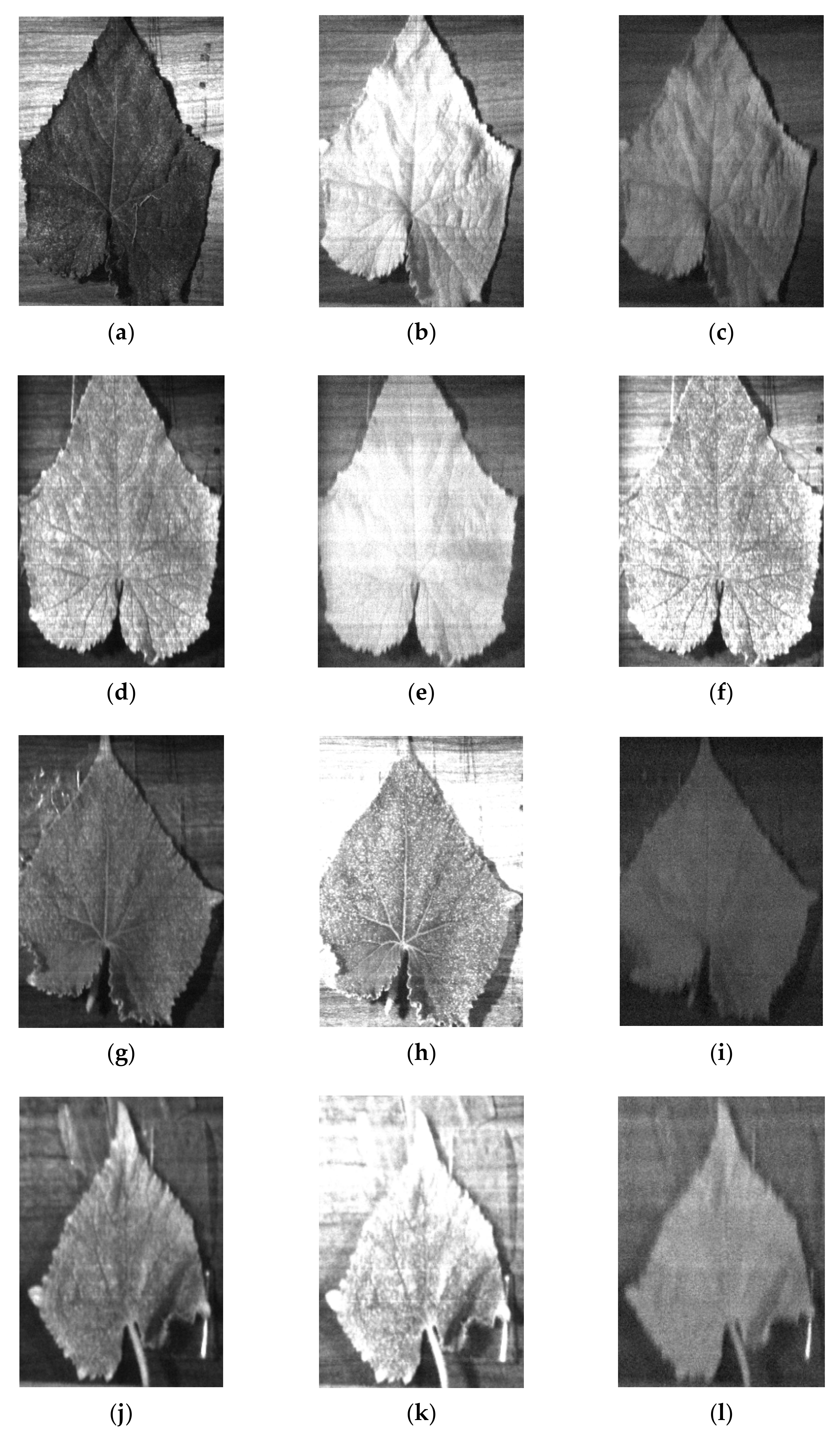
3.5. Sample Images and Comparison with Other Works

Some examples of the hyperspectral images of two classes of leaves with normal nitrogen fertilizer (D0) and leaves with excess nitrogen (D1) at two spectral ranges of visible (Vis) and near-infrared (NIR) light are shown in Figure 11. As can be seen, on the first day after applying excess nitrogen, the contaminated pixels were not detectable in the visible range. However, at the NIR range there were white pixels clearly visible at the edges of the leaf that represented excess nitrogen consumption. In other words, if classical spectral analysis were applied to the entire leaf, the detection of overapplication would be done at a later stage, since the negative effects start at the tips of the leaves. By using spectral images, the problems can be detected earlier.

After assessing the performance of the proposed algorithm, the results were compared with other methods conducted by different researchers.

Table 9. Comparison of the results obtained in this study with other research.

Method	Product Type	Early Detection Type	CCR (%)
Proposed method	Cucumber	Excess nitrogen	96.11
[40]	Tomato	Gray mold disease	94.44–97.22
[41]	Prawns	Freshness	95.0–98.33
[42]	Honey	Adulteration	84.0–95.0
[43]	Oilseed rape	Waterlogging stress	94.44–95.9
[44]	Wheat	Insects	96.7
[45]	Wheat	Fungi	94.6
[46]	Bell peppers	Bruises	94.9

compares the results of these methods using the reported values of classification accuracy (or CCR).

It must be observed that the problems addressed in these papers and the product types are different, since no comparable works have been found in the literature regarding the detection of excess nitrogen in cucumber leaves. Therefore, this information is offered to compare our results with other state-of-the-art work in HSI processing. The accuracy of the proposed method, above 96%, is comparable with or better than most of these previous techniques. Another important advantage of HSI with respect to traditional spectral analysis is that it enables automation of the image acquisition process. Although in the current experiment, the images were obtained in a capture chamber, it is possible to mount such cameras on drones or satellites. In this way, after obtaining the images, a leaf detector could be applied to find the leaves and then analyze the nitrogen content on each one of them. This is not possible if spatial information is not available. However, the problems derived from natural lighting and uncontrolled conditions should be addressed, which pose a challenge in NIR spectral analysis.

4. Conclusions

In recent years, agricultural producers have increased the use of chemical fertilizers per unit of area, instead of using modern agricultural knowledge to produce more. The illusion of increasing yield due to the use of more water and chemical fertilizers has led to the excessive use of water and fertilizer resources. The continuation of these practices has led, in some countries, to situations of soil and water contamination, in addition to additional expenses.

Hyperspectral imaging (HSI) has been recognized as a non-destructive and rapid analytical tool for evaluating product quality and diagnosing diseases using new technological advances in data measurement. In the present study, a new HSI methodology was proposed to evaluate early detection of excess nitrogen consumption in cucumber plants, complemented with computational intelligence methods using hybrid approaches of artificial neural networks (ANN) and metaheuristic algorithms (ABC and ICA). First, using the hybrid ANN-ABC algorithm, the wavelengths of 715, 773 and 821 nm were determined as the key wavelengths to analyze nitrogen in the leaves. The hybrid approach ANN-ICA was then applied to predict the number of days of treatment using the HSI data in the selected wavelengths.

The performance of the proposed classifier was evaluated using the confusion matrix and the ROC curves. The total correct classification rate achieved was 96.11%, indicating a good ability to detect excess nitrogen in cucumber plants. The statistical analysis showed that the differences between the images of the selected wavelengths for the different days of treatment were statistically significant.

By early detection of excess fertilizer, nitrogen-rich soil can be improved. One of the ways to improve the soil with excess nitrogen is by applying mulch. The nitrogen-rich soil of mulch decomposes large amounts of soil nitrogen. The proposed technique can be used to adjust the use of nitrogen to the optimum values, thus reducing the use of fertilizers and the risk of contamination.

One of the limitations of the proposed method is that it requires specialized imaging equipment, although the processing can be done on an average computer. The high cost of this equipment would not be affordable for most farmers. In the future, with the development of specialized cameras in the selected wavelengths, it will be possible to estimate the nitrogen content of the plants using images taken in the field, thus maintaining it at optimal levels. For this purpose, new challenges derived from the use of natural lighting conditions should be addressed. Another future research line would be to study different levels of nitrogen lower than 30% so that the system would be more sensitive to detect small excesses in the use of fertilizers.

References

1. Blasco, J.; Aleixos, N.; Cubero, S.; Gómez-Sanchís, J.; Moltó, E. Automatic sorting of satsuma (Citrus unshiu) segments using computer vision and morphological features. Comput. Electron. Agric. 2009, 66, 1–8. [Google Scholar] [CrossRef]
2. Pourdarbani, R.; Sabzi, S.; García-Amicis, V.M.; García-Mateos, G.; Molina-Martínez, J.M.; Ruiz-Canales, A. Automatic Classification of Chickpea Varieties Using Computer Vision Techniques. Agronomy 2019, 9, 672. [Google Scholar] [CrossRef] [Green Version]
3. Paliwal, J.; Shashidhar, N.S.; Jayas, D.S. Grain kernel identification using kernel signature. Trans. ASAE 1999, 42, 1921–1924. [Google Scholar] [CrossRef]
4. Paliwal, J.; Visen, N.; Jayas, D.; White, N. Cereal Grain and Dockage Identification using Machine Vision. Biosyst. Eng. 2003, 85, 51–57. [Google Scholar] [CrossRef]
5. Pourdarbani, R.; Sabzi, S.; Hernández-Hernández, M.; Hernández-Hernández, J.L.; García-Mateos, G.; Kalantari, D.; Molina-Martínez, J.M. Comparison of Different Classifiers and the Majority Voting Rule for the Detection of Plum Fruits in Garden Conditions. Remote Sens. 2019, 11, 2546. [Google Scholar] [CrossRef] [Green Version]
6. Sabzi, S.; Javadikia, P.; Rabbani, H.; Adelkhani, A.; Naderloo, L. Exploring the best model for sorting blood orange using ANFIS method. Agric. Eng. Int. CIGR J. 2013, 15, 213–219. [Google Scholar]
7. Pourdarbani, R.; Sabzi, S.; Kalantari, D.; Hernández-Hernández, J.L.; Arribas, J.I. A Computer Vision System Based on Majority-Voting Ensemble Neural Network for the Automatic Classification of Three Chickpea Varieties. Foods 2020, 9, 113. [Google Scholar] [CrossRef] [PubMed] [Green Version]
8. Lu, J.; Li, W.; Yu, M.; Zhang, X.; Ma, Y.; Su, X.; Yao, X.; Cheng, T.; Zhu, Y.; Cao, W.; et al. Estimation of rice plant potassium accumulation based on non-negative matrix factorization using hyperspectral reflectance. Precis. Agric. 2021, 22, 51–74. [Google Scholar] [CrossRef]
9. Mahesh, S.; Jayas, D.; Paliwal, J.; White, N. Hyperspectral imaging to classify and monitor quality of agricultural materials. J. Stored Prod. Res. 2015, 61, 17–26. [Google Scholar] [CrossRef]
10. Salimi, M.; Pourdarbani, R.; Nouri, B.A. Factors Affecting the Adoption of Agricultural Automation Using Davis’s Acceptance Model (Case Study: Ardabil). Acta Technol. Agric. 2020, 23, 30–39. [Google Scholar] [CrossRef] [Green Version]
11. Rehman, A.U.; Qureshi, S.A. A review of the medical hyperspectral imaging systems and unmixing algorithms’ in biological tissues. Photodiagnosis Photodyn. Ther. 2021, 33, 102165. [Google Scholar] [CrossRef] [PubMed]
12. Li, Z.; Zhang, Q.; Li, J.; Yang, X.; Wu, Y.; Zhang, Z.; Wang, S.; Wang, H.; Zhang, Y. Solar-induced chlorophyll fluorescence and its link to canopy photosynthesis in maize from continuous ground measurements. Remote. Sens. Environ. 2020, 236, 111420. [Google Scholar] [CrossRef]
13. Abdulridha, J.; Batuman, O.; Ampatzidis, Y. UAV-Based Remote Sensing Technique to Detect Citrus Canker Disease Utilizing Hyperspectral Imaging and Machine Learning. Remote. Sens. 2019, 11, 1373. [Google Scholar] [CrossRef] [Green Version]
14. Hu, J.; Zhao, M.; Li, Y. Hyperspectral Image Super-Resolution by Deep Spatial-Spectral Exploitation. Remote Sens. 2019, 11, 1229. [Google Scholar] [CrossRef] [Green Version]
15. Feng, W.; Qi, S.; Heng, Y.; Zhou, Y.; Wu, Y.; Liu, W.; He, L.; Li, X. Canopy Vegetation Indices from In situ Hyperspectral Data to Assess Plant Water Status of Winter Wheat under Powdery Mildew Stress. Front. Plant Sci. 2017, 8, 1219. [Google Scholar] [CrossRef]
16. Zheng, H.; Cheng, T.; Yao, X.; Deng, X.; Tian, Y.; Cao, W.; Zhu, Y. Detection of rice phenology through time series analysis of ground-based spectral index data. Field Crop. Res. 2016, 198, 131–139. [Google Scholar] [CrossRef]
17. Stroppiana, D.; Boschetti, M.; Brivio, P.A.; Bocchi, S. Plant nitrogen concentration in paddy rice from field canopy hyperspectral radiometry. Field Crop. Res. 2009, 111, 119–129. [Google Scholar] [CrossRef]
18. Xiaobo, Z.; Jiyong, S.; Limin, H.; Jiewen, Z.; Hanpin, M.; Zhenwei, C.; Yanxiao, L.; Holmes, M. In vivo noninvasive detection of chlorophyll distribution in cucumber (Cucumis sativus) leaves by indices based on hyperspectral imaging. Anal. Chim. Acta 2011, 706, 105–112. [Google Scholar] [CrossRef] [PubMed]
19. Ning, J.; Sun, J.; Li, S.; Sheng, M.; Zhang, Z. Classification of five Chinese tea categories with different fermentation degrees using visible and near-infrared hyperspectral imaging. Int. J. Food Prop. 2016, 20, 1–8. [Google Scholar] [CrossRef] [Green Version]
20. Huang, L.; Zhao, J.; Chen, Q.; Zhang, Y. Rapid detection of total viable count (TVC) in pork meat by hyperspectral imaging. Food Res. Int. 2013, 54, 821–828. [Google Scholar] [CrossRef]
21. Del Fiore, A.; Reverberi, M.; Ricelli, A.; Pinzari, F.; Serranti, S.; Fabbri, A.A.; Bonifazi, G.; Fanelli, C. Early detection of toxigenic fungi on maize by hyperspectral imaging analysis. Int. J. Food Microbiol. 2010, 144, 64–71. [Google Scholar] [CrossRef]
22. Singh, C.B.; Jayas, D.S.; Paliwal, J.; White, N.D.G. Fungal Detection in Wheat Using Near-Infrared Hyperspectral Imaging. Trans. ASABE 2007, 50, 2171–2176. [Google Scholar] [CrossRef]
23. Ghosal, S.; Blystone, D.; Singh, A.K.; Ganapathysubramanian, B.; Singh, A.; Sarkar, S. An explainable deep machine vision framework for plant stress phenotyping. Proc. Natl. Acad. Sci. USA 2018, 115, 4613–4618. [Google Scholar] [CrossRef] [Green Version]
24. Shamshiri, R.R.; Hameed, I.A.; Balasundram, S.K.; Ahmad, D.; Weltzien, C.; Yamin, M. Fundamental Research on Unmanned Aerial Vehicles to Support Precision Agriculture in Oil Palm Plantations. Agric. Robot. Fundam. Appl. 2019, 91–116. [Google Scholar] [CrossRef] [Green Version]
25. Audebert, N.; Le Saux, B.; Lefèvre, S. Deep Learning for Classification of Hyperspectral Data: A Comparative Review. IEEE Geosci. Remote Sens. Mag. 2019, 7, 159–173. [Google Scholar] [CrossRef] [Green Version]
26. Balasubramaniam, P.; Ananthi, V.P. Segmentation of nutrient deficiency in incomplete crop images using intuitionistic fuzzy C-means clustering algorithm. Nonlinear Dyn. 2016, 83, 849–866. [Google Scholar] [CrossRef]
27. Backhaus, A.; Bollenbeck, F.; Seiffert, U. High-throughput quality control of coffee varieties and blends by artificial neural networks and hyperspectral imaging. In Proceedings of the 1st International Congress on Cocoa, Coffee and Tea (CoCoTea), Novara, Italy, 13–16 September 2011. [Google Scholar]
28. Condori, R.H.M.; Romualdo, L.M.; Bruno, O.M.; Luz, P.H.D.C. Comparison Between Traditional Texture Methods and Deep Learning Descriptors for Detection of Nitrogen Deficiency in Maize Crops. In Proceedings of the 2017 Workshop of Computer Vision (WVC), Natal, Brazil, 30 October–1 November 2017; pp. 7–12. [Google Scholar]
29. Mogollón, R.; Contreras, C.; Neta, M.L.D.S.; Marques, E.J.N.; Zoffoli, J.P.; De Freitas, S.T. Non-destructive prediction and detection of internal physiological disorders in ’Keitt’ mango using a hand-held Vis-NIR spectrometer. Postharvest Biol. Technol. 2020, 167, 111251. [Google Scholar] [CrossRef]
30. Dezordi, L.R.; de Aquino, L.A.; de Almeida Aquino, R.F.B.; Clemente, J.M.; Assunção, N.S. Diagnostic Methods to Assess the Nutritional Status of the Carrot Crop. Rev. Bras. Ciência Solo 2016, 40. [Google Scholar] [CrossRef]
31. Ma, L.; Fang, J.; Chen, Y.; Gong, S. Color Analysis of Leaf Images of Deficiencies and Excess Nitrogen Content in Soybean Leaves. In Proceedings of the 2010 International Conference on E-Product E-Service and E-Entertainment, Henan, China, 7–9 November 2010; pp. 1–3. [Google Scholar]
32. Yang, Z.O.; Mei, X.; Gao, F.; Li, Y.; Guo, J. Effect of Different Nitrogen Fertilizer Types and Application Measures on Temporal and Spatial Variation of Soil Nitrate-Nitrogen at Cucumber Field. J. Environ. Prot. 2013, 4, 129–135. [Google Scholar] [CrossRef] [Green Version]
33. Pham, D.T.; Ghanbarzadeh, A.; Koc, E.; Otri, S.; Rahim, S.; Zaidi, M. The Bees Algorithm; Technical Note; Manufacturing Engineering Centre, Cardiff University: Cardiff, UK, 2005. [Google Scholar]
34. Hussain, A.; Zhang, M.; Üçpunar, H.K.; Svensson, T.; Quillery, E.; Gompel, N.; Ignell, R.; Kadow, I.C.G. Ionotropic Chemosensory Receptors Mediate the Taste and Smell of Polyamines. PLoS Biol. 2016, 14, e1002454. [Google Scholar] [CrossRef] [PubMed]
35. Wang, W.; Paliwal, J. Spectral Data Compression and Analyses Techniques to Discriminate Wheat Classes. Trans. ASABE 2006, 49, 1607–1612. [Google Scholar] [CrossRef]
36. Rossel, R.A.V. ParLeS: Software for chemometric analysis of spectroscopic data. Chemom. Intell. Lab. Syst. 2008, 90, 72–83. [Google Scholar] [CrossRef]
37. Kjeldahl, J. Neue Methode zur Bestimmung des Stickstoffs in organischen Körpern. Anal. Bioanal. Chem. 1883, 22, 366–382. [Google Scholar] [CrossRef] [Green Version]
38. Atashpaz-Gargari, E.; Lucas, C. Imperialist competitive algorithm: An algorithm for optimization inspired by imperialistic competition. In Proceedings of the 2007 IEEE Congress on Evolutionary Computation, Singapore, 25–28 September 2007. [Google Scholar] [CrossRef]
39. Pourdarbani, R.; Sabzi, S.; Kalantari, D.; Karimzadeh, R.; Ilbeygi, E.; Arribas, J.I. Automatic non-destructive video estimation of maturation levels in Fuji apple (Malus Malus pumila) fruit in orchard based on colour (Vis) and spectral (NIR) data. Biosyst. Eng. 2020, 195, 136–151. [Google Scholar] [CrossRef]
40. Xie, C.; Yang, C.; He, Y. Hyperspectral imaging for classification of healthy and gray mold diseased tomato leaves with different infection severities. Comput. Electron. Agric. 2017, 135, 154–162. [Google Scholar] [CrossRef]
41. Dai, Q.; Cheng, J.-H.; Sun, D.-W.; Pu, H.; Zeng, X.-A.; Xiong, Z. Potential of visible/near-infrared hyperspectral imaging for rapid detection of freshness in unfrozen and frozen prawns. J. Food Eng. 2015, 149, 97–104. [Google Scholar] [CrossRef]
42. Shafiee, S.; Polder, G.; Minaei, S.; Moghadam-Charkari, N.; Van Ruth, S.; Kuś, P.M. Detection of Honey Adulteration using Hyperspectral Imaging. IFAC-PapersOnLine 2016, 49, 311–314. [Google Scholar] [CrossRef]
43. Xia, J.; Cao, H.; Yang, Y.; Zhang, W.; Wan, Q.; Xu, L.; Ge, D.; Zhang, W.; Ke, Y.; Huang, B. Detection of waterlogging stress based on hyperspectral images of oilseed rape leaves (Brassica napus L.). Comput. Electron. Agric. 2019, 159, 59–68. [Google Scholar] [CrossRef]
44. Paliwal, J.; Wang, W.; Symons, S.J.; Karunakaran, C. Insect species and infestation level determination in stored wheat using near-infrared spectroscopy. Can. Biosyst. Eng. 2004, 46, 17–24. [Google Scholar]
45. Zhang, H.; Paliwal, J.; Jayas, D.S.; White, N.D.G. Classification of Fungal Infected Wheat Kernels Using Near-Infrared Reflectance Hyperspectral Imaging and Support Vector Machine. Trans. ASABE 2007, 50, 1779–1785. [Google Scholar] [CrossRef]
46. Babellahi, F.; Paliwal, J.; Erkinbaev, C.; Amodio, M.L.; Chaudhry, M.M.A.; Colelli, G. Early detection of chilling injury in green bell peppers by hyperspectral imaging and chemometrics. Postharvest Biol. Technol. 2020, 162, 111100. [Google Scholar] [CrossRef]
Figure 1. Different stages of the proposed methodology for classifying cucumber plant nitrogen content. ANN-ABC: artificial neural networks and artificial bee colony algorithm. ANN-ICA: artificial neural networks and imperialist competitive algorithm.
Agronomy 11 00575 g001
Figure 2. Overview of the cucumber pots used in the experiments.
Agronomy 11 00575 g002
Figure 3. Hardware configuration of the capture system: (a) hyperspectral camera; (b) illumination chamber.
Agronomy 11 00575 g003
Figure 4. Some examples of the hyperspectral images of cucumber leaves in the range of wavelengths from 400 to 1100 nm: (a) 420 nm; (b) 540 nm; (c) 690 nm; (d) 800 nm; (e) 950 nm; (f) 1040 nm.
Agronomy 11 00575 g004aAgronomy 11 00575 g004b
Figure 5. Some original and pre-processed spectral diagrams of different samples using ParLeS software, version 3.1.
Agronomy 11 00575 g005
Figure 7. Hyperspectral images of the selected wavelengths during the sampling days. Left column (a,d,g,j): 715 nm; middle column (b,e,h,k): 783 nm; right column (c,f,i,l): 821 nm. Rows: days since the excess nitrogen started, from top to bottom: D0 (ac), D1 (df), D2 (gi) and D3 (jl), respectively.
Agronomy 11 00575 g007
Figure 8. Box plots of the performance of the ANN-ICA classifier for the 200 repetitions: (a) correct classification rate (CCR); (b) area under the receiver operating characteristic (ROC) curve (AUC) for each class; AUCD0, AUCD1, AUCD2 and AUCD3 correspond to Days 0, 1, 2 and 3, respectively.
Agronomy 11 00575 g008
Figure 9. ROC curves of the ANN-ICA classifier at 200 repetitions for the four classes.
Agronomy 11 00575 g009
Figure 10. ROC curves of the ANN-ICA classifier for the four classes for the best training case.
Agronomy 11 00575 g010
Figure 11. Sample images of the cucumber leaves at different wavelengths. Upper row (a,b): without treatment (D0); lower row (c,d): after 1 day of application of excess nitrogen (D1). Left column (a,c): wavelength in the visible band (582 nm); right column (b,d): wavelength in the near-infrared range (NIR) band (908 nm).
Agronomy 11 00575 g011