
Evaluation of Injection Strategies in Supersonic Nozzle Flow


1
Department of Fluid-Flow Machinery, TU Wien, Getreidemarkt 9, 1060 Vienna, Austria
2
Department of Mechanics, Royal Institute of Technology (KTH), Osquars Backe 18, 10044 Stockholm, Sweden
*
Author to whom correspondence should be addressed.
Aerospace 2021, 8(12), 369; https://doi.org/10.3390/aerospace8120369
Submission received: 26 October 2021
/
Revised: 18 November 2021
/
Accepted: 26 November 2021
/
Published: 29 November 2021
(This article belongs to the Section Aeronautics)
Abstract
:The ability to manipulate shock patterns in a supersonic nozzle flow with fluidic injection is investigated numerically using Large Eddy Simulations. Various injector configurations in the proximity of the nozzle throat are screened for numerous injection pressures. We demonstrate that fluidic injection can split the original, single shock pattern into two weaker shock patterns. For intermediate injection pressures, a permanent shock structure in the exhaust can be avoided. The nozzle flow can be manipulated beneficially to increase thrust or match the static pressure at the discharge. The shock pattern evolution of injected stream is described over various pressure ratios. We find that the penetration depth into the supersonic crossflow is deeper with subsonic injection. The tight arrangement of the injectors can provoke additional counter-rotating vortex pairs in between the injection.
1. Introduction
A wide range of engineering applications capitalises on the benefits of fluidic injection into supersonic crossflows, e.g., flame-holding [1], thrust vectoring [2], supersonic air-breathing engines, and noise suppression [3,4]. The shock wave pattern associated with such high-speed applications has been described experimentally [5,6,7,8,9], and numerically using steady-state RANS calculations [10] and Large Eddy Simulations (LES) [11,12,13]. Multiple jets in crossflow have been used in gas turbine combustors [14] and shock wave translation [4,15].
Semlitsch & Mihăescu [16] applied multiple injection into nozzle crossflows to manipulate the shock pattern of supersonic exhausts using steady-state RANS simulations. A location slightly downstream from the nozzle throat with an inclination angle of was found to be optimal to reduce the shock wave strength. Morris et al. [17] used fluidic injection into a convergent–divergent nozzle to reduce screech and shock associated broadband noise. Even though the observation of noise reduction and numerous fundamental studies of a jet in crossflow have been made, it could not be identified why and when the internal fluidic injection is beneficial. Further, the understanding of the mutual influence of injected streams is limited especially in supersonic flow regimes where flow and shock structures interact. With this investigation, we shade light into the effects of fluidic injection into a supersonic convergent–divergent nozzle flow using the LES approach, where we focus on a beneficial location identified by Semlitsch & Mihăescu [16].
Flow Structure Generation with Jet Injection into Supersonic Crossflow
The interaction of injection and crossflow provokes intrinsic vortical flow structures, such as horseshoe vortices [10,11], hanging vortices [11,18], shear-layer vortices, and the counter-rotating vortex pair. Besides the injection and crossflow Reynolds numbers, the appearance of the jet in crossflow phenomena have been classified accordingly to the non-dimensional effective velocity ratio, ,
representing the square root of the momentum flux ratio. u is the velocity, is the density, is the specific heat ratio, p is the static pressure, and M is the Mach number. The subscript j relates the quantity to the injected jet, whereas references to the crossflow. The ratio of the incoming boundary layer thickness, , to the injection pipe diameter, is another dimensionless parameter classifying the horseshoe vortex evolution [19]. The incident boundary layer influences the flow structure generation at the orifice of the injection pipe, while its diameter governs the actual interfacial area between the jet and the crossflow. The amplified flow disturbances propagating in the turbulent boundary layer lead to a faster breakdown of the coherent shear-layer flow structures. Consequentially, the turbulent boundary layer increases the mixing rate, and coherent flow structures do not evolve as evident in high-speed as in low-speed flows. In supersonic flow, Genin & Menon [11], and Kawai & Lele [12] did not observe distinct shedding frequencies, which was linked to the turbulent inflow conditions.
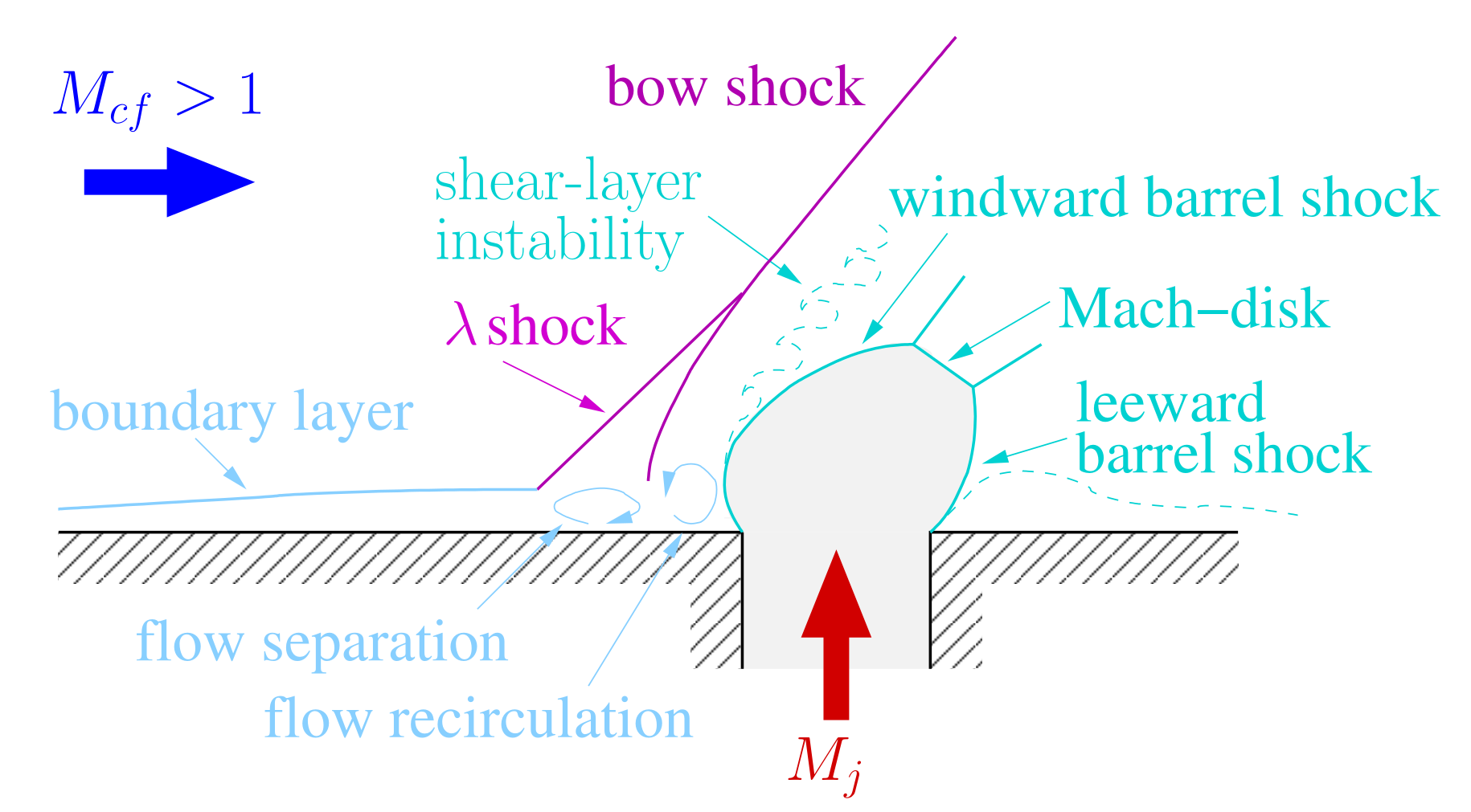
The supersonic injection comes with shock patterns, as exemplary sketched in Figure 1. The non-pressure matched sonic injection expands into the crossflow forming a Prandtl-Meyer expansion fan and a following barrel shock structure with Mach-disk. Kawai & Lele [12], and Genin & Menon [11] investigated the barrel shock motion and found that the windward barrel shock exhibits large scale motion, whereas the leeward barrel shock side remains static. Vortical structures shedding in the jet windward shear-layer cause the windward barrel shock to follow their motion. With the motion of the windward barrel shock, acoustic waves are emitted. These perturbations significantly displace the bow shock forming upstream of the injection [20]. Papamoschou & Hubbard [20] and Viti et al. [10] reported a flow recirculation region underneath the bow shock.
2. Materials and Methods
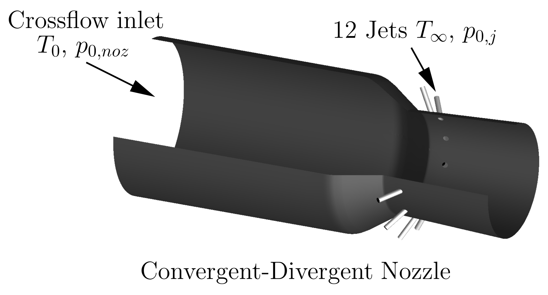
The considered geometry consists of an axisymmetric convergent–divergent nozzle, which is illustrated in Figure 2. Twelve cylindrical pipes, inclined to the nozzle centre-axis, are arranged equidistantly on its circumference in the divergent section. The design Mach number at the nozzle exit is , and the area ratio is , which is defined as the nozzle exit area to the throat cross-sectional area . A total pressure source, , drives the nozzle flow, which is four times the ambient pressure . The employed total temperature at the domain inlet is set slightly higher than the ambient temperature to mimic the operating conditions of the experimental measurements at the University of Cincinnati [21] and allow thereby direct comparison of the results. Downstream of the nozzle exit, the stream expands into a quiescent ambient environment. The applied boundary conditions are summarised in Table 1.
Three injection locations , i.e., , , and upstream from the nozzle exit, are considered to investigate the sensitivity of the shock pattern on the injection location found beneficial by Semlitsch & Mihăescu [16]. The injector diameter is of mm. The injector total temperature is set to the ambient temperature, and the flow is aligned with the pipe axis. The injector total pressure is an investigation parameter referred to as Injection Pressure Ratio (IPR), relating the applied total pressure at the injector inlet to the ambient pressure.
2.1. Numerical Simulation Procedure
The three-dimensional nozzle flow is simulated by solving the Navier–Stokes equations for compressible fluids numerically, which can be written as,
where t is the time, the spatial coordinates, is the fluid density, u the velocity, p the static pressure defined by the ideal gas law, , and the viscous stress tensor. For a Newtonian media, the viscous stress tensor can be written as,
where is the Kronecker delta, is the dynamic viscosity, and is the strain rate tensor. The temperature dependence of the dynamic viscosity, , is modelled using Sutherland’s formula,
where is the reference dynamic viscosity, is the reference temperature, and is the Sutherland temperature. The values set for the constants are; kg/s m, 273.15 , and 110.4 . The strain rate tensor can be defined as,
The conservation of mass and energy is guaranteed, by solving the conservation equations
and
respectively, where is the total internal energy and is the heat flux. The total internal energy can be linked to the other primary variables by,
The heat flux is calculated by employing Fourier’s law,
where K is the heat conductivity.
An explicit low-storage four-stage Runge–Kutta scheme of second-order accuracy was utilised for temporal integration. A constant time-step was set for time advancement to satisfy the Courant–Friedrichs–Lewy condition (see Table 2). The inviscid flux is computed for finite volumes using a second-order central difference scheme, where a Jameson-type artificial dissipation [22] is added to avoid spurious numerical oscillations near sharp gradients or discontinuities, such as shock waves. The added dissipation is based on a blend of second and fourth-order differences triggered by a pressure difference sensor. The viscous stresses in the governing equations can be expressed by a vector Laplacian of the flow-field. The identity of the Laplacian equation is used to calculate the second-order gradient terms. The remaining terms for a fully viscous approach are obtained using a Green–Gauss formulation. Thereby, a second-order accurate discretisation for the viscous terms is achieved. A more detailed description of the utilised solver, edge, has been provided by Eliasson [23].
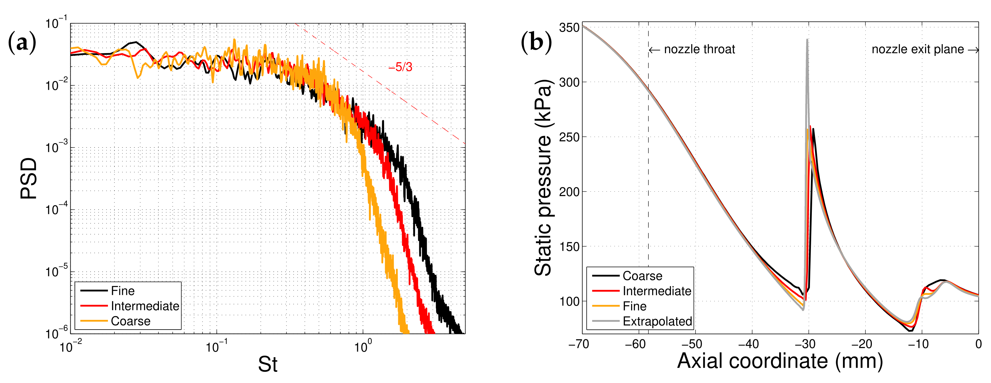
The smallest flow scales, i.e., shock wave thickness or smallest turbulent length scales, are lower than a mesh resolution with efficient use of computational resources could handle. Thus, the governing equations are spatially filtered, and the Favre-averaging of the equation set is performed. The arising subgrid-scale terms account for unresolved physics. The nature of the smallest flow scales is to dissipate the kinetic energy into heat at the molecular level. This effect needs to be endorsed employing some model since insufficient dissipation would promote an unphysical energy build up [24]. Smagorinsky [25] introduced an artificial viscosity model, similar to the eddy viscosity concept, acting as a subgrid-scale model to stabilise the numerical approach. Calibration coefficients are required, which can affect the flow-field substantially, e.g., shown by Uzun et al. [26], and need to be obtained empirically. Despite the recent development of novel subgrid-scale models [27,28,29], the compressible nature of nozzle flow challenges the choice of an adequate explicit subgrid-scale model. At a distance from solid walls, the dissipation is dominated by the kinetic energy transfer from the large to the small flow scales. This behaviour is statistically universal at sufficiently high Reynolds number accordingly to Kolmogorov’s hypothesis, which is promising for modelling. In the present approach, the subgrid scales are represented implicitly by the intrinsic numerical dissipation of the solver. The approach is also known as monotonically integrated Large Eddy Simulation or implicit LES. For a non-oscillatory finite volume discretisation of at least second-order accuracy, the numerical truncation error can be interpreted as a Clark-type subgrid-scale model for the momentum equation and as a Smagorinsky-type subgrid-scale model for the energy conservation Equation [30]. Hence, the kinetic energy fluctuations are absolutely decreasing with this approach and no spurious energy build-up at the high frequencies occurs, which is proven by the spectra shown in Figure 3a. The entire discretisation resolution of the mesh grid is exploited, and no information is truncated by an explicit filter [31,32]. Further, no calibration constants are required, which might be difficult to obtain for internal supersonic nozzle flows.
2.2. Meshes, Verification and Validation
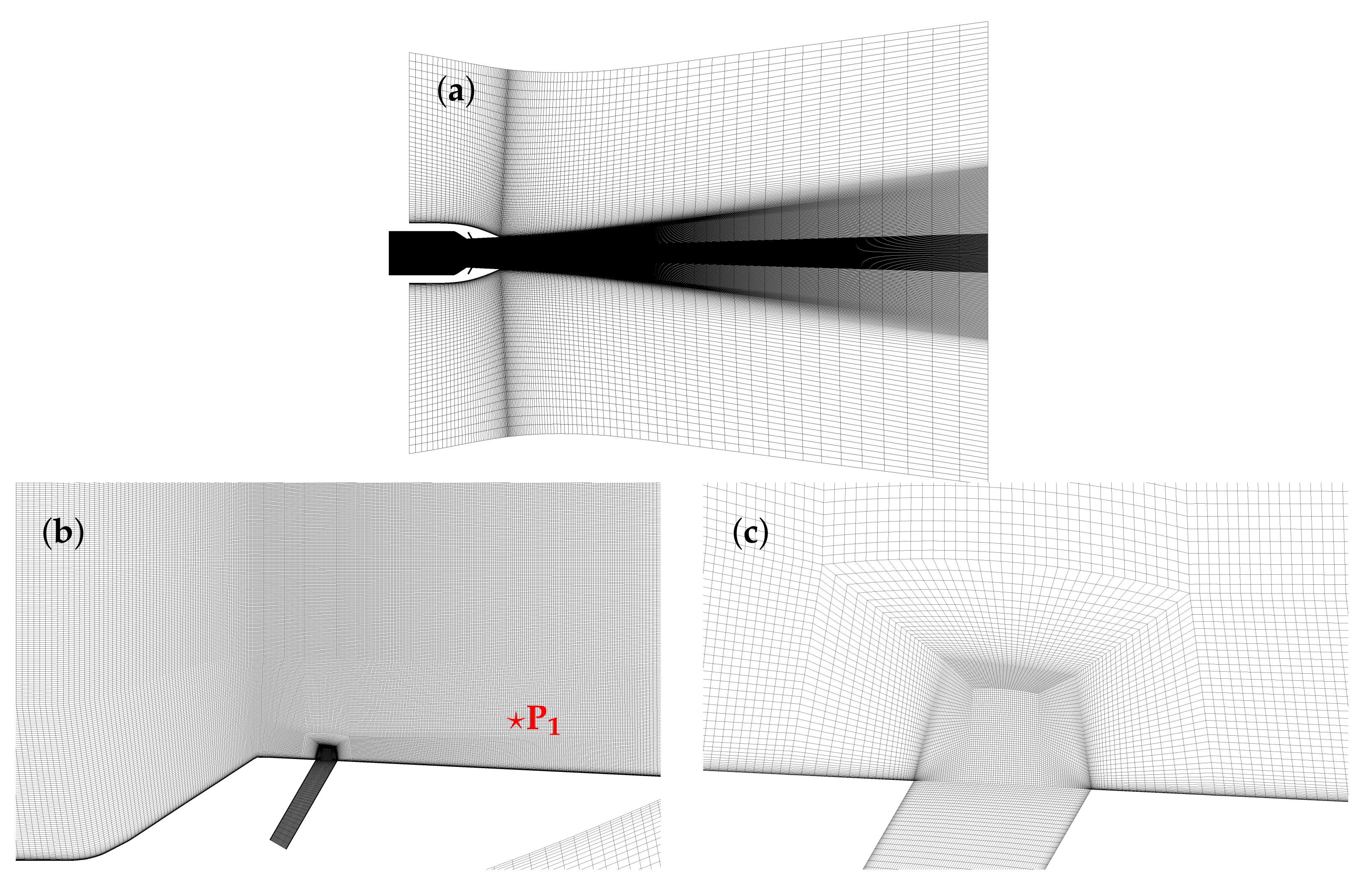
The numerical grids consist of 259 hexahedral blocks arranged in a centred O-structure, which is shown in Figure 4. The discretisations of all injectors are structured with an individual O-grid to enable consistent near-wall refinement. The mesh in the investigation section is retained to be as uniformly fine spaced as possible. The inlet and outlet sections assist to buffer undesired reflections by gradual cell size increments the boundary conditions. The buffer region downstream of the nozzle exit covers an expansion zone into stagnant ambient conditions.
A mesh resolution study was performed using three grid levels while conserving the block structure. The specific properties of the meshes are listed in Table 2. Figure 3a illustrates the velocity spectra obtained from static pressure signal recorded in the probe , which is located in the wake of the injection as indicated in Figure 4b. The spectra reveal the same broadband content at low frequencies (consistent with the reported results by Kawai & Lele [12], and Genin & Menon [11]), while the captured turbulent cascade is prolonged with the mesh refinement.
The methodology suggested by Celik et al. [33] has been chosen to analyse the effect of grid refinement quantitatively, which is based on the Richardson extrapolation. The numerical solution obtained on three grid levels is extrapolated to an infinite fine grid, and the resulting error is assessed. For an injection pressure ratio of at the intermediate jet injection location (i.e., on the divergent slope of the nozzle at upstream from the nozzle exit), the solutions of the estimated static pressure on the nozzle centreline with three grids and the Richardson extrapolation are shown in Figure 3b. The solutions show nearly overlapping contours in the smooth flow-field regions and a shift (in the order of a mesh cell) of the shock wave in the upstream direction with increased mesh resolution.
Table 3 shows that the mean relative error between intermediate and fine grid is small, although the maximal relative error is high. Shock waves represent steep discontinuous gradients, which induce even for a small shift a large maximal relative error. The relative errors between the numerical solution and the extrapolation are even lower (as shown in Table 3), which suggests that the grids are properly designed to capture shock pattern changes with fluidic injection accurately.
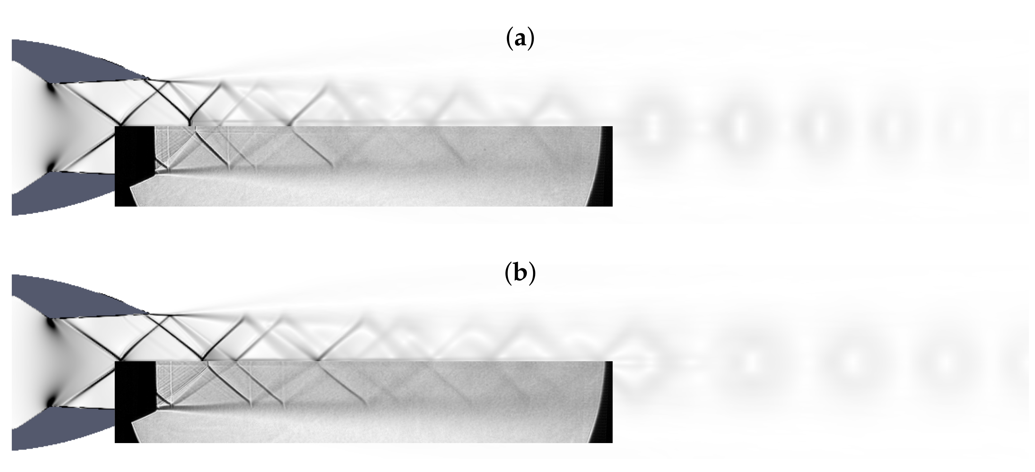
The experimental visualisation of confined supersonic flow is challenging. Instead, the numerical simulation data are compared to measurements of the external shock pattern performed at the University of Cincinnati [34]. Figure 5 reveals that the numerical approach captures (on a coarser mesh resolution than the intermediate mesh) accurately the shock wave angles and locations, which are the focus of the present investigation. More quantitative validation with particle image velocimetry data has been documented by Semlitsch et al. [4] for external fluidic injection, where a good agreement regarding the streamwise velocity magnitudes and shock wave angles and locations are reported.
3. Results
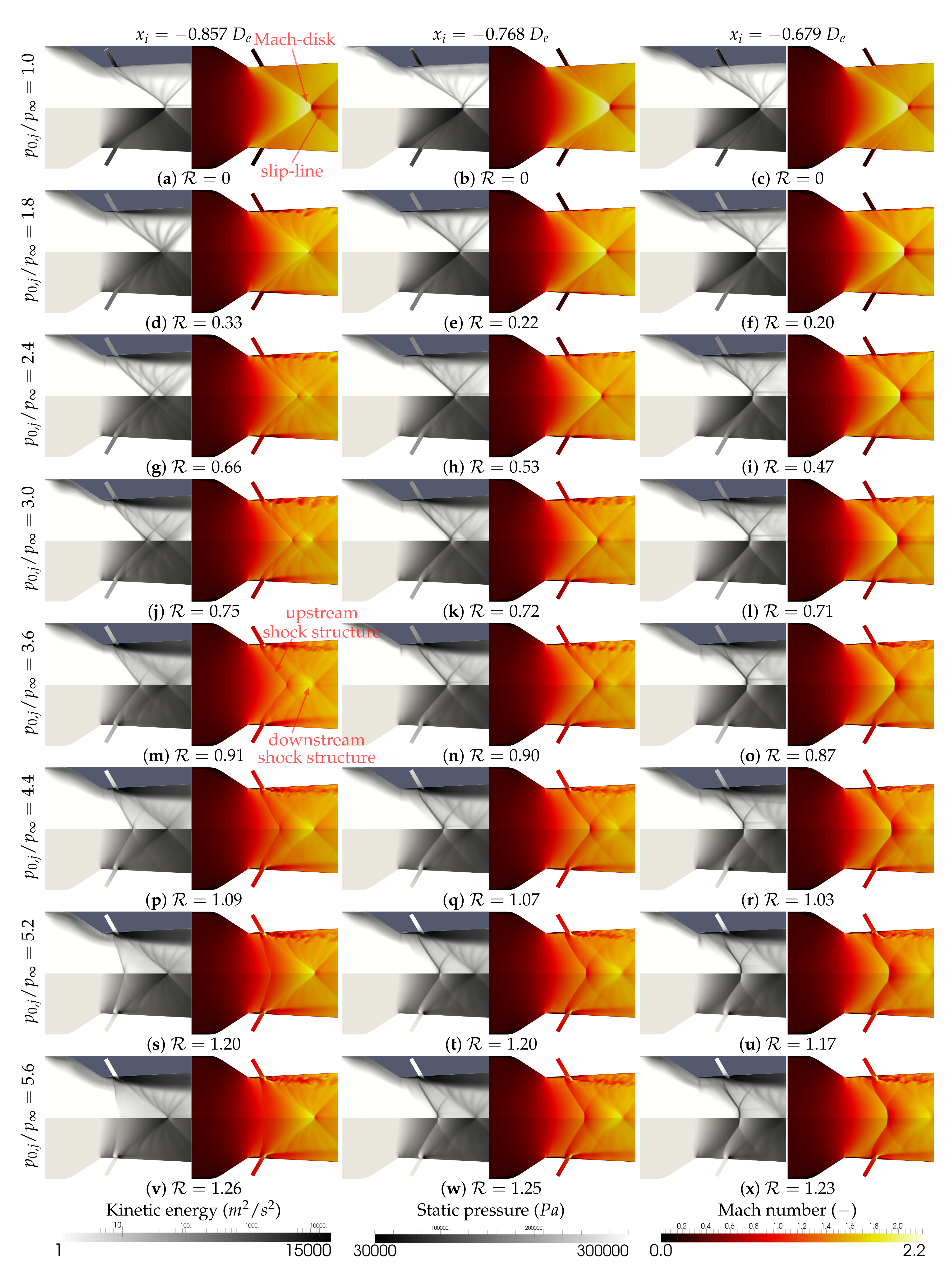
Figure 6 illustrates the shock pattern transformation in the divergent nozzle section for different injection pressures and locations. We define the shock pattern occurring without injection as the baseline, where an oblique shock anchors slightly downstream of the nozzle throat and merges in the core in the form of a Mach-disk. There, shock wave reflections and slip-lines arise. This shock structure can be split into two separate employing fluidics. Bow shocks establish upstream of the injection governing the shock structure. A second shock structure establishes on top of the injected flow. The upstream shock structure steepens with increasing injection pressure, and the downstream shock structure shifts the nozzle exit.
The oblique shock angle, , is governed by the pressure ratio across it, the upstream Mach number, , and the ratio of specific heats, ,
where the indices 1 and 2 refer to the quantities to the upstream and downstream locations, respectively. Figure 6 shows that the static pressure distributions (without injection) differ on the nozzle circumference for the individual injection locations. As a consequence, the crossflow momentum is there different, which pushes against the injected stream. The force balance of the injected flow momentum blocking the crossflow induces locally high static pressure regions at the injector orifice (for all ). The mass flow rate and the effective velocity ratios, , develop differently for individual injector configurations with equal IPRs accordingly to the static pressure at the injector orifice. The pressure ratio over the bow shock increases with increasing IPR. This also amplifies the static pressure downstream of the bow shock continuation, and the angle of the first upstream shock structure steepens.
The flow accelerates in the divergent nozzle section until hitting the first upstream shock. Hence, the further downstream the first upstream shock is situated, the higher the upstream Mach number, , and the lower the upstream static pressure, , of the shock. The pressure downstream of the first upstream shock, , is governed by the injection. The pressure ratio is too high for an oblique shock, and a Mach disk establishes for the downstream injection location. On the contrary, the flow did not accelerate enough to reach low enough pressures to support a normal shock wave for the upstream injection location.
The fluidic injection contracts the core flow. Thereby, the penetration depth governs the location of the second downstream shock structure. For low injection pressure ratios, the injected jets remain attached to the nozzle walls. The kinetic energy fluctuations indicate that once the injection separates from the nozzle walls, the penetration depth into the crossflow scales with the effective velocity ratio, , until the injectors choke (). The radial penetration ceases beyond choke.
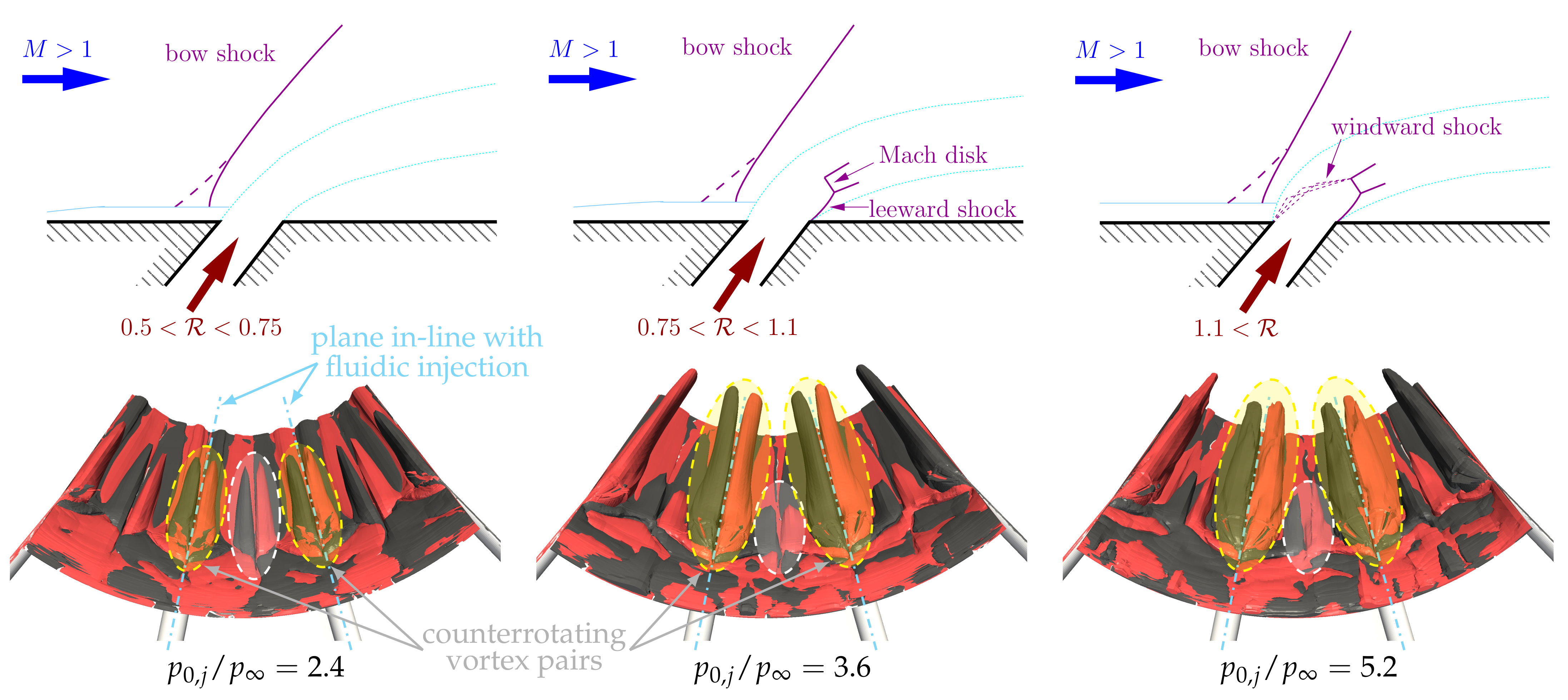
The evolution of the injection shock pattern with increased is sketched in Figure 7. The injection remains subsonic for below . A leeward shock arises for separating the injected jet and the flow recirculation downstream of it. Mach disks appear spontaneously on top of the leeward shock. The crossflow shears the windward side of the injection, and windward shocks do not emerge until reaches . These windward shocks remain weak and exhibit intense motion. Genin & Menon [11], and Kawai & Lele [12] simulated higher effective velocity ratios and observed that this motion of the shocks in the injection causes vortex breakdown or bursting.
Figure 7 shows the counterrotating vortex pairs in terms of streamwise vorticity iso-surfaces, which reveal a lower penetration depth in radial direction for injection with shocks () than injection with sporadic shocks (). The counterrotating vortex pair results relatively weak for , but an additional counterrotating vortex pair establishes in between the injection (highlighted in white in Figure 7). In proximity to the nozzle wall, the nozzle flow is diverted and partially forced in between the injection. Thereby, the incoming stream is contracted and pushed partially away from the walls. Such an additional counterrotating vortex pair can also be observed for other injector operating conditions but evolves less clearly due to the enhanced unsteadiness.
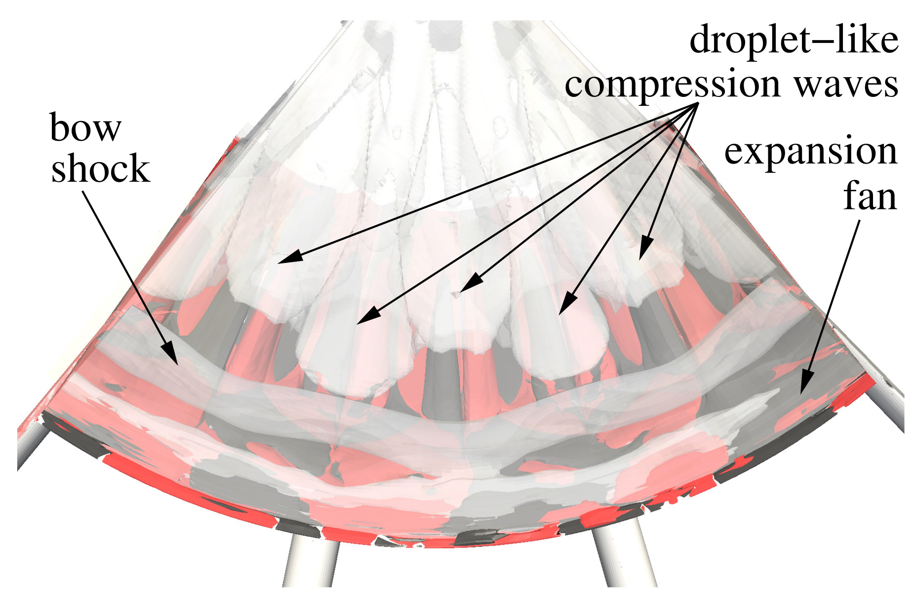
Several compression waves form the second downstream shock structure (see Figure 6). Illustrating the time-averaged pressure fluctuations as transparent iso-surface on top of the counterrotating vortex pair in Figure 8 demonstrates that the compression waves anchor on the injected stream. Especially for higher injection pressure ratios, these compression waves display strong motion as the kinetic energy fluctuations show in Figure 6, which is related to the injection unsteadiness. For intermediate injection pressure ratios (3.0–4.4) at the upstream and intermediate injection location, compression waves cannot always focus as a second downstream shock pattern (the transient behaviour of the compression waves can be observed in the animation provided as Supplementary Material.). It is noteworthy that the first upstream shock structure is not reflected (at all times), and therefore, the exhaust remains without persistent shock waves.
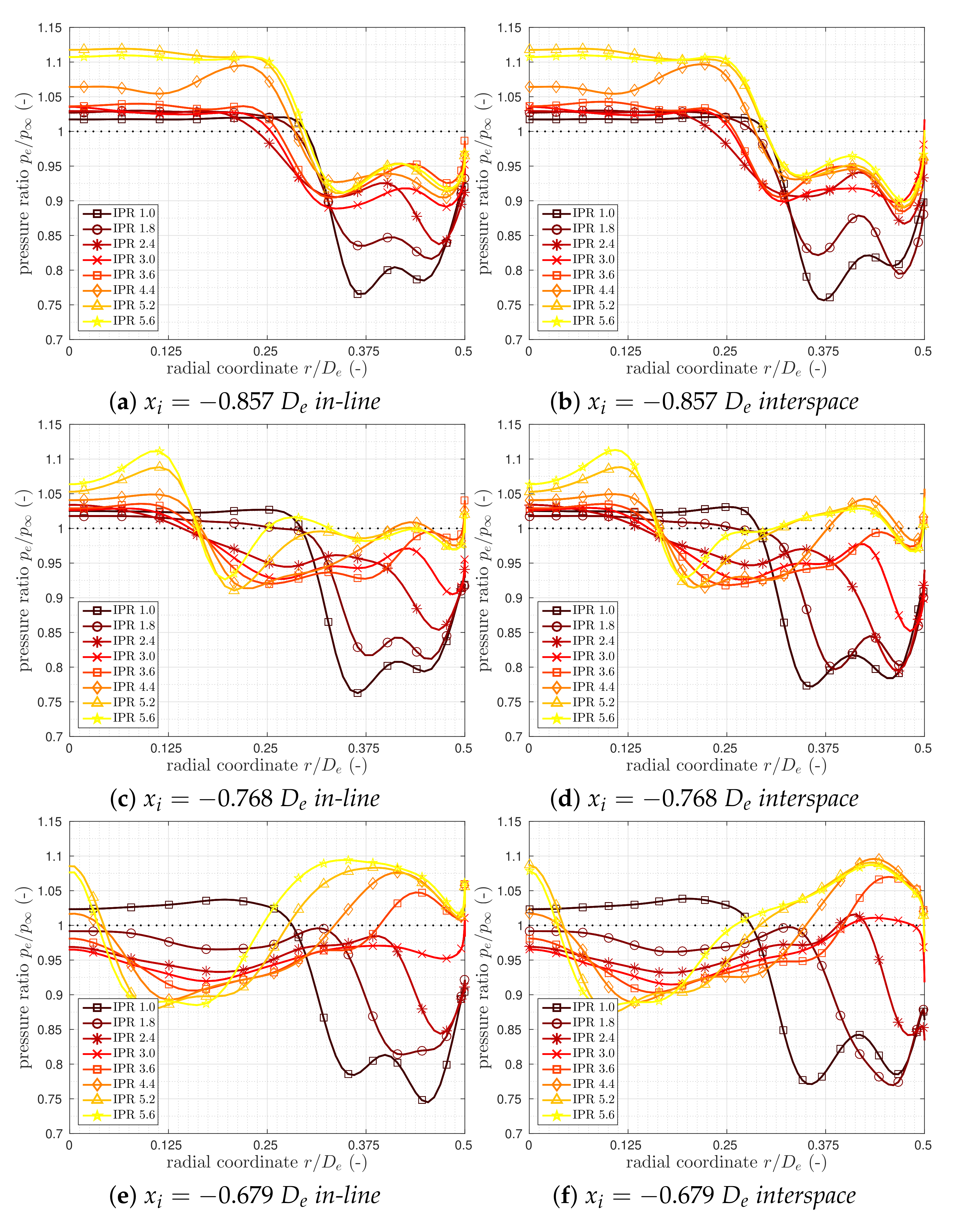
Fluidics can be potentially used to compensate for the under-expansion of an exhausting jet and match the static with the ambient pressure at the nozzle exit. The profiles of the time-averaged static pressures shown in Figure 9 exhibit significant radial variations at the nozzle exit, which can be attributed to the shock waves and injected wakes penetrating this plane. Without fluidic injection, the static pressure is high in the interior flow while being significantly lower at the outer circumference. Figure 9 demonstrates that injection augments the static pressure successively at the circumference, where the injection location affects its impact. Significant differences between the wake and in between wake profiles can only be noted for the most downstream injection location. Hence, the injected flow is not the principal contributor to the static pressure rise at the circumference. Moreover, the downstream shift of the second, downstream shock pattern towards the nozzle exit is the cause. The best pressure match (uniform around the circumference) is achieved for injection pressure ratios of approximately for the intermediate injection location.
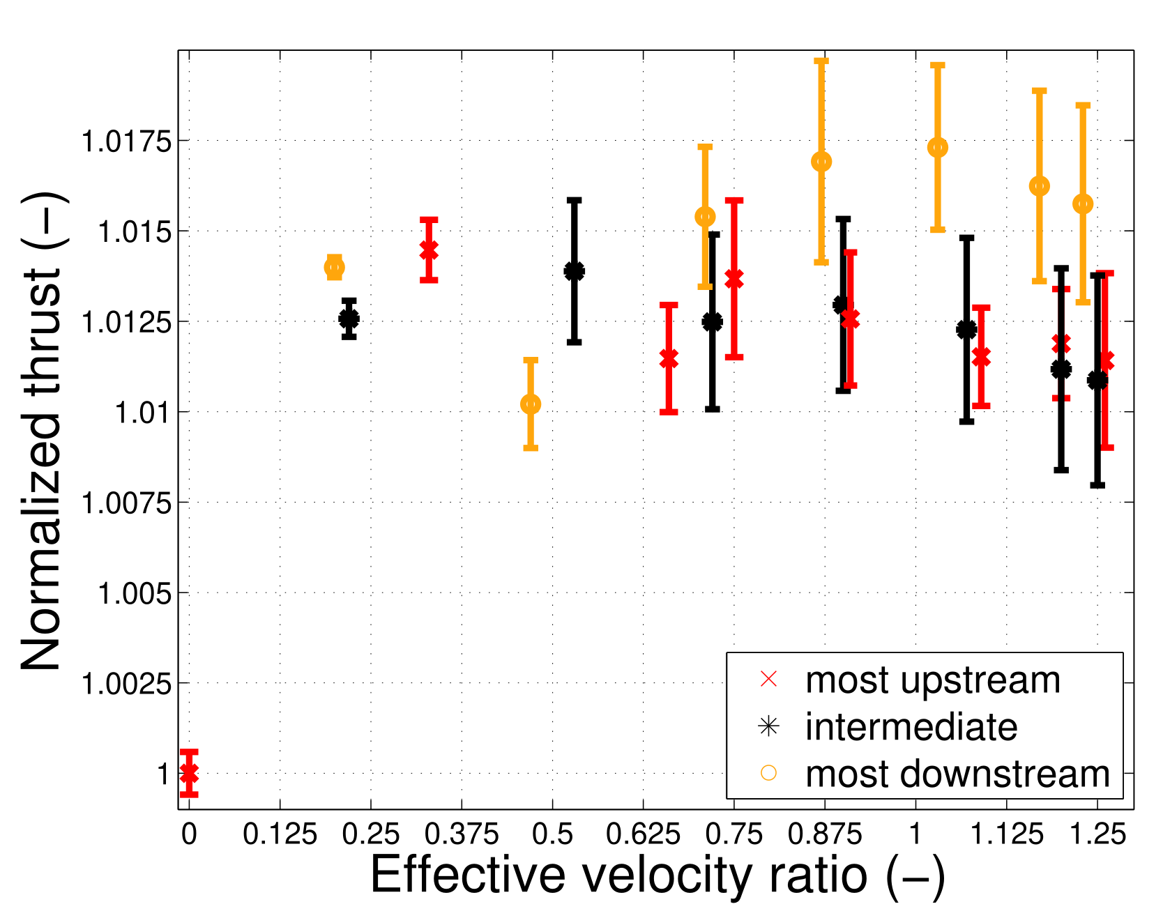
Shock, mixing and blockage losses reduce the nozzle efficiency to generate thrust. The mean and variance of the thrust (samples over simulation time) are illustrated in Figure 10. Even low injection amounts increase the thrust, while a little additional benefit is achieved with higher injection pressures. This is not unexpected because the nozzle is operating an underexpanded exhaust, as shown in Figure 5.
Figure 6 shows that the Mach-disk is most extensive for the downstream injection configuration. Although the most considerable shock associated losses may be expected for this configuration (neglecting bow shock losses), the thrust is the highest, as revealed by Figure 10. (the cross-sectional area of the Mach-disk remains small compared to the total cross-section.) The high thrust results are due to the high flow velocities in the core flow and beneficial static pressures at the circumference for this configuration. Thus, shifting the shock pattern is more beneficial for thrust optimisation than shock strength reduction.
The thrust variance can be reduced using fluidics with low injection pressure ratios, i.e., . The injection introduces unsteadiness in the divergent nozzle section for higher injection pressures. The generated thrust unsteadiness arises from induced shock pattern motion rather than the flow unsteadiness in the injection wakes.
4. Conclusions
The ability to transform shock patterns in convergent–divergent nozzles with fluidic injection has been investigated using Large Eddy Simulations. The numerical approach has been validated with Shadowgraph visualisations, and the uncertainty due to the grid resolution has been assessed. We showed that fluidics could transform a single shock pattern manifesting in a converged-divergent nozzle into two weaker shock structures. The bow shocks (upstream of the injection) form the first shock structure, and a second shock structure establishes on top of the penetrating injection. The first upstream shock pattern steepens with increased injection amount, while the second shock pattern location shifts downstream. The sensitivity of the shock pattern to injection pressure changes is linked to the injection location. The surface static pressure is lowest towards the nozzle throat. Consequentially, higher mass flow rates arise for injection close to the nozzle throat, which causes deeper injection penetration. Once the injected jets choke, the shock waves compensate partially for the pressure difference.
It was shown that even low injection pressures augment the thrust, compensating for the underexpanded nozzle operating condition. The most favourable injection configuration was found when a (second downstream) shock pattern was shifted towards the nozzle exit plane. Although the shock associated losses are high for this configuration, the high core-flow velocities in combination with high static pressures at the nozzle circumference generate the highest thrust.
The closely spaced fluidic injection can provoke additional counter-rotating vortex pairs in between injectors. The generated vorticity forms the source of the additional established counter-rotating vortex pairs within the injection ports for some of the injection pressure ratios considered. The formation of additional counter-rotating vortex pairs was linked with compression waves forming in between the upstream shock wave and the consecutive shock wave reflection.
We have shown that the shock pattern could be transformed into a transient compression wave pattern for some injection configurations. The compression waves exhibited intense motion and did focus only at times to a shock pattern. The fluidic injection can also be used to match the static pressure at the nozzle exit plane for over-expanded exhausts to evade shock formation at the nozzle exit. We find that the injection pressure is not of primary importance to achieve pressure distributions favouring ideal expanded operating conditions at the nozzle exit. The shift of the shock pattern inside of the nozzle is the critical parameter. Hence, shock associated noise can be attenuated most efficiently using internal fluidic injection, as demonstrated by Morris et al. [17] and Cuppoletti et al. [21].
Supplementary Materials
The Supplementary Materials are available online at https://www.mdpi.com/article/10.3390/aerospace8120369/s1.
Author Contributions
Conceptualisation, B.S.; methodology, B.S.; validation, B.S.; investigation, B.S.; data curation, B.S.; writing—original draft preparation, B.S.; writing—review and editing, B.S. and M.M.; supervision, M.M. All authors have read and agreed to the published version of the manuscript.
Funding
The authors would like to acknowledge the Swedish Defense Materiel Administration (FMV) for financial support for this research through the grant; 311956-A1 722654. This work was supported by the Swedish National Infrastructure for Computing (SNIC 002-12-11 & SNIC 2013-11-19) via HPC2N and PDC.
Data Availability Statement
Not applicable.
Acknowledgments
Ephraim J. Gutmark and Daniel Cuppoletti from the University of Cincinnati are acknowledged for providing experimental data used in this study to validate the numerical results.
Conflicts of Interest
The authors declare no conflict of interest.
Abbreviations
The following nomenclature and abbreviations are used in this manuscript:
| Abbreviations | |
| LES | Large Eddy Simulation |
| IPR | Injection Pressure Ratio |
| RANS | Reynolds-Averaged Navier–Stokes |
| Latin symbols | |
| e | specific internal energy () |
| p | pressure () |
| q | heat flux () |
| t | time (s) |
| u | velocity |
| x | axial coordinate (m) |
| A | area () |
| D | diameter (m) |
| K | heat conductivity () |
| M | Mach number (−) |
| apparent order (−) | |
| R | specific gas constant () |
| effective velocity ratio (−) | |
| strain rate tensor () | |
| Strouhal number (-) | |
| T | temperature (K) |
| Greek symbols | |
| shock wave inclination angle (rad) | |
| ratio of the specific heats (-) | |
| boundary layer thickness (m) | |
| Kronecker delta function (−) | |
| relative error (%) | |
| dynamic viscosity () | |
| density () | |
| viscous shear stress tensor (Pa) |
| Superscript | |
| average | |
| narrowest cross-section | |
| Subscript | |
| 0 | stagnation or total quantity state |
| ∞ | ambient quantity state |
| variable is referred to the crossflow | |
| e | variable is referenced to the nozzle exit |
| j | variable is referred to injection or injector |
| constant is referred to as reference value | |
| constant of Sutherland’s formula | |
| variable is referred to nozzle inlet |
References
- Ben-Yakar, A.; Hanson, R. Experimental investigation of flame-holding capability of hydrogen transverse jet in supersonic cross-flow. In Symposium (International) on Combustion; Elsevier: Amsterdam, The Netherlands, 1998; Volume 27, pp. 2173–2180. [Google Scholar] [CrossRef]
- Strykowski, P.; Krothapalli, A.; Forliti, D. Counterflow thrust vectoring of supersonic jets. AIAA J. 1996, 34, 2306–2314. [Google Scholar] [CrossRef]
- Henderson, B. Fifty years of fluidic injection for jet noise reduction. Int. J. Aeroacoust. 2010, 9, 91–122. [Google Scholar] [CrossRef]
- Semlitsch, B.; Cuppoletti, D.; Gutmark, E.; Mihăescu, M. Transforming the Shock Pattern of Supersonic Jets using Fluidic Injection. AIAA J. 2019, 57, 1851–1861. [Google Scholar] [CrossRef] [Green Version]
- Lee, M.; McMillin, B.; Palmer, J.; Hanson, R. Planar fluorescence imaging of a transverse jet in a supersonic crossflow. J. Propuls. Power 1992, 8, 729–735. [Google Scholar] [CrossRef]
- Santiago, J.G.; Dutton, J.C. Velocity measurements of a jet injected into a supersonic crossflow. J. Propuls. Power 1997, 13, 264–273. [Google Scholar] [CrossRef]
- Tomioka, S.; Jacobsen, L.S.; Schetz, J.A. Sonic injection from diamond-shaped orifices into a supersonic crossflow. J. Propuls. Power 2003, 19, 104–114. [Google Scholar] [CrossRef]
- Beresh, S.J.; Henfling, J.F.; Erven, R.J.; Spillers, R.W. Penetration of a transverse supersonic jet into a subsonic compressible crossflow. AIAA J. 2005, 43, 379–389. [Google Scholar] [CrossRef]
- Beresh, S.J.; Henfling, J.F.; Erven, R.J.; Spillers, R.W. Crossplane velocimetry of a transverse supersonic jet in a transonic crossflow. AIAA J. 2006, 44, 3051–3061. [Google Scholar] [CrossRef]
- Viti, V.; Neel, R.; Schetz, J.A. Detailed flow physics of the supersonic jet interaction flow field. Phys. Fluids 2009, 21, 046101. [Google Scholar] [CrossRef]
- Génin, F.; Menon, S. Dynamics of sonic jet injection into supersonic crossflow. J. Turbul. 2010, 11, N4. [Google Scholar] [CrossRef]
- Kawai, S.; Lele, S.K. Large-eddy simulation of jet mixing in supersonic crossflows. AIAA J. 2010, 48, 2063–2083. [Google Scholar] [CrossRef]
- Mousavi, S.M.; Roohi, E. Large eddy simulation of shock train in a convergent–divergent nozzle. Int. J. Mod. Phys. C 2014, 25, 1450003. [Google Scholar] [CrossRef] [Green Version]
- Holdeman, J.D.; Walker, R. Mixing of a Row of Jets with a Confined Crossflow. AIAA J. 1977, 15, 243–249. [Google Scholar] [CrossRef]
- Verma, S.; Manisankar, C. Shockwave/Boundary-Layer Interaction Control on a Compression Ramp Using Steady Micro Jets. AIAA J. 2012, 50, 2753–2764. [Google Scholar] [CrossRef]
- Semlitsch, B.; Mihăescu, M. Fluidic Injection Scenarios for Shock Pattern Manipulation in Exhausts. AIAA J. 2018, 56, 4640–4644. [Google Scholar] [CrossRef]
- Morris, P.J.; McLaughlin, D.K.; Kuo, C.W. Noise reduction in supersonic jets by nozzle fluidic inserts. J. Sound Vib. 2013, 332, 3992–4003. [Google Scholar] [CrossRef]
- Yuan, L.L.; Street, R.L.; Ferziger, J.H. Large-eddy simulations of a round jet in crossflow. J. Fluid Mech. 1999, 379, 71–104. [Google Scholar] [CrossRef]
- Kelso, R.; Smits, A. Horseshoe vortex systems resulting from the interaction between a laminar boundary layer and a transverse jet. Phys. Fluids 1995, 7, 153–158. [Google Scholar] [CrossRef]
- Papamoschou, D.; Hubbard, D. Visual observations of supersonic transverse jets. Exp. Fluids 1993, 14, 468–476. [Google Scholar] [CrossRef]
- Cuppoletti, D.; Gutmark, E.; Hafsteinsson, H.; Eriksson, L.E. Elimination of Shock-Associated Noise in Supersonic Jets by Destructive Wave Interference. AIAA J. 2019, 57, 720–734. [Google Scholar] [CrossRef]
- Jameson, A.; Schmidt, W.; Turkel, E. Numerical solutions of the Euler equations by finite volume methods using Runge–Kutta time-stepping schemes. In Proceedings of the 14th Fluid and Plasma Dynamics Conference, Palo Alto, CA, USA, 23–25 June 1981; Volume 81, p. 1259. [Google Scholar] [CrossRef] [Green Version]
- Eliasson, P. A Navier–Stokes Solver for Unstructured Grids. In FOI/FFA Report FOIR-0298-SE, FOI; Swedish Defence Research Agency: Stockholm, Sweden, 2001. [Google Scholar]
- Verstappen, R. How much eddy dissipation is needed to counterbalance the nonlinear production of small, unresolved scales in a large-eddy simulation of turbulence? Comput. Fluids 2018, 176, 276–284. [Google Scholar] [CrossRef]
- Smagorinsky, J. The beginnings of numerical weather prediction and general circulation modeling: Early recollections. Adv. Geophys. 1983, 25, 3–37. [Google Scholar] [CrossRef]
- Uzun, A.; Blaisdell, G.A.; Lyrintzis, A.S. Sensitivity to the Smagorinsky constant in turbulent jet simulations. AIAA J. 2003, 41, 2077–2079. [Google Scholar] [CrossRef]
- Maulik, R.; San, O.; Jacob, J.D.; Crick, C. Sub-grid scale model classification and blending through deep learning. J. Fluid Mech. 2019, 870, 784–812. [Google Scholar] [CrossRef] [Green Version]
- Zahiri, A.P.; Roohi, E. Anisotropic minimum-dissipation (AMD) subgrid-scale model implemented in OpenFOAM: Verification and assessment in single-phase and multi-phase flows. Comput. Fluids 2019, 180, 190–205. [Google Scholar] [CrossRef]
- Zhou, H.; Li, X.; Qi, H.; Yu, C. Subgrid-scale model for large-eddy simulation of transition and turbulence in compressible flows. Phys. Fluids 2019, 31, 125118. [Google Scholar]
- Margolin, L.G.; Rider, W.J. A rationale for implicit turbulence modelling. Int. J. Numer. Methods Fluids 2002, 39, 821–841. [Google Scholar] [CrossRef]
- Fureby, C.; Grinstein, F. Monotonically integrated large eddy simulation of free shear flows. AIAA J. 1999, 37, 544–556. [Google Scholar] [CrossRef]
- Grinstein, F.F.; Fureby, C. Recent progress on MILES for high Reynolds number flows. J. Fluids Eng. 2002, 124, 848–861. [Google Scholar] [CrossRef]
- Celik, I.B.; Ghia, U.; Roache, P.J.; Freitas, C.J. Procedure for estimation and reporting of uncertainty due to discretization in CFD applications. J. Fluids Eng. 2008, 130, 078001. [Google Scholar] [CrossRef] [Green Version]
- Munday, D.; Heeb, N.; Gutmark, E.; Burak, M.; Eriksson, L.E.; Prisell, E. Forward flight effects on the shock structure from a chevron C-D nozzle. In Proceedings of the 48th AIAA Aerospace Sciences Meeting Including the New Horizons Forum and Aerospace Exposition, Orlando, FL, USA, 4–7 January 2010. [Google Scholar]
Figure 1.
The shock pattern structure with jet in supersonic crossflow.

Figure 2.
Geometry and set-up.

Figure 3.
The effect of grid refinement is illustrated comparing the streamwise velocity spectra obtained in probe location (a) and the static pressure on the centreline (b).
Figure 3.
The effect of grid refinement is illustrated comparing the streamwise velocity spectra obtained in probe location (a) and the static pressure on the centreline (b).

Figure 4.
The numerical grid is shown in a mid-plane view; entire computational domain (a), zoomed view of the investigation section (b), and detailed view at the interface between a jet pipe and nozzle surface (c).
Figure 4.
The numerical grid is shown in a mid-plane view; entire computational domain (a), zoomed view of the investigation section (b), and detailed view at the interface between a jet pipe and nozzle surface (c).

Figure 5.
Numerical schlieren, i.e., the density gradient magnitude, images are compared to experimental shadowgraph images. (a) , (b) .
Figure 5.
Numerical schlieren, i.e., the density gradient magnitude, images are compared to experimental shadowgraph images. (a) , (b) .

Figure 6.
Left column: the kinetic energy fluctuations and time-averaged static pressure contours are shown on the top and bottom half, respectively. Right column: the instantaneous and time-averaged Mach number contours are plotted on the top and lower half, respectively. The effective velocity ratios, , are specified.

Figure 7.
Top row: sketch of the shock pattern appearance as function of in-line with the fluidic injection. Lower row: time-averaged streamwise vorticity iso-surfaces looking towards the nozzle exit (red and black colour represent positive and negative streamwise vorticity, respectively).
Figure 7.
Top row: sketch of the shock pattern appearance as function of in-line with the fluidic injection. Lower row: time-averaged streamwise vorticity iso-surfaces looking towards the nozzle exit (red and black colour represent positive and negative streamwise vorticity, respectively).

Figure 8.
The time-averaged streamwise vorticity iso-surfaces are shown for for a quarter section of the nozzle. On top, iso-surfaces of the pressure fluctuation are plotted to indicate the location of shock waves and compression waves.
Figure 8.
The time-averaged streamwise vorticity iso-surfaces are shown for for a quarter section of the nozzle. On top, iso-surfaces of the pressure fluctuation are plotted to indicate the location of shock waves and compression waves.

Figure 9.
Effect of injection pressure and location: radial time-averaged static pressure profiles (normalised by the ambient pressure) are shown at the nozzle exit, in-line with injection (in-line: (a,c,e)) and in between the injection (interspace: (b,d,f)), respectively.
Figure 9.
Effect of injection pressure and location: radial time-averaged static pressure profiles (normalised by the ambient pressure) are shown at the nozzle exit, in-line with injection (in-line: (a,c,e)) and in between the injection (interspace: (b,d,f)), respectively.

Figure 10.
Thrust estimations where the variance is represented by errorbars.


Table 1.
Reference values and operating conditions.
| Parameter | Symbol | Value | Unit |
|---|---|---|---|
| nozzle inlet diameter | |||
| nozzle exit diameter | |||
| nozzle area ratio | (-) | ||
| nozzle design Mach number | (-) | ||
| nozzle pressure ratio | 4 | (-) | |
| nozzle inlet temperature | 367 | ||
| injector pipe diameter | |||
| injector inclination angle | 60 | ||
| ambient pressure | 101,325 | ||
| ambient temperature | 288.15 |
Table 2.
Mesh attributes; total number of cells, wall next cell height , average cell size in the investigation region, and the time step .
Table 2.
Mesh attributes; total number of cells, wall next cell height , average cell size in the investigation region, and the time step .
| Number of Cells | min | |||
|---|---|---|---|---|
| I | 11 million | 1.0 × m | m | s |
| II | 22 million | m | m | s |
| III | 44 million | m | m | s |
Table 3.
Key values of the grid resolution study using the Richardson extrapolation, where the mean, minimal, and maximal values of the relative error between fine and intermediate mesh , the apparent order , the relative error between extrapolated solution and fine mesh, and grid convergence index are listed.
| mean | ||||
| min | 6.4 | |||
| max |
Publisher’s Note: MDPI stays neutral with regard to jurisdictional claims in published maps and institutional affiliations. |
© 2021 by the authors. Licensee MDPI, Basel, Switzerland. This article is an open access article distributed under the terms and conditions of the Creative Commons Attribution (CC BY) license (https://creativecommons.org/licenses/by/4.0/).
Share and Cite
MDPI and ACS Style
Semlitsch, B.; Mihăescu, M. Evaluation of Injection Strategies in Supersonic Nozzle Flow. Aerospace 2021, 8, 369. https://doi.org/10.3390/aerospace8120369
AMA Style
Semlitsch B, Mihăescu M. Evaluation of Injection Strategies in Supersonic Nozzle Flow. Aerospace. 2021; 8(12):369. https://doi.org/10.3390/aerospace8120369
Chicago/Turabian StyleSemlitsch, Bernhard, and Mihai Mihăescu. 2021. "Evaluation of Injection Strategies in Supersonic Nozzle Flow" Aerospace 8, no. 12: 369. https://doi.org/10.3390/aerospace8120369
Note that from the first issue of 2016, this journal uses article numbers instead of page numbers. See further details here.