Application of an Efficient Gradient-Based Optimization Strategy for Aircraft Wing Structures


1
School of Mechanical and Aerospace Engineering, Queen’s University Belfast, Belfast BT9 5AH, Northern Ireland, UK
2
Engineering Design Centre, Department of Engineering, University of Cambridge, Cambridge CB2 1PZ, UK
3
School of Aerospace, Transport and Manufacturing, Cranfield University, Cranfield Mk43 0AL, UK
*
Author to whom correspondence should be addressed.
Aerospace 2018, 5(1), 3; https://doi.org/10.3390/aerospace5010003
Submission received: 8 December 2017
/
Revised: 26 December 2017
/
Accepted: 2 January 2018
/
Published: 4 January 2018
(This article belongs to the Special Issue Feature Papers in Aerospace)
Abstract
:In this paper, a practical optimization framework and enhanced strategy within an industrial setting are proposed for solving large-scale structural optimization problems in aerospace. The goal is to eliminate the difficulties associated with optimization problems, which are mostly nonlinear with numerous mixed continuous-discrete design variables. Particular emphasis is placed on generating good initial starting points for the search process and in finding a feasible optimum solution or improving the chances of finding a better optimum solution when traditional techniques and methods have failed. The efficiency and reliability of the proposed strategy were demonstrated through the weight optimization of different metallic and composite laminated wingbox structures. The results show the effectiveness of the proposed procedures in finding an optimized solution for high-dimensional search space cases with a given level of accuracy and reasonable computational resources and user efforts. Conclusions are also inferred with regards to the sensitivity of the optimization results obtained with respect to the choice of different starting values for the design variables, as well as different optimization algorithms in the optimization process.
1. Introduction
Optimization methods play a key role in aerospace structural design; their very purpose is to find the most optimal way for an engineer to obtain the utmost benefit from the available resources. Structural optimization methods evolved in the aerospace industry in the late 1950s, when the need to design lightweight structures was critical [1,2,3]. Since then, the aerospace manufacturing industry has shown increasing interest in the application of optimization methods for the optimum design of minimum-weight aircraft structural components [4,5,6]. There is a large number of publications on the structural optimization of aircraft. A few of these key studies are referenced in this section to provide the reader with some background information on the field. In the 1960s, Brandt and Wasiutynski [7] reviewed the present state of knowledge in the field of optimal design of structures. In addition, survey papers by Schmit [8] and Vanderplaats [9] offered numerous and important references on the theory and applications of structural optimization. The development of structural optimization methods can be tracked to the early works of Maxwell [10] and Michell [11]. In the 1940s and early 1950s, substantial analytical work was done on component optimization, of which the work presented by Shanley [12] is a typical example. Dantzig [13] developed linear programming techniques, and with the advent of computer technology, these techniques were applied to the design of frame and beam structures, as explained by Heyman [14]. In his work, Schmit [15] offered a comprehensive study on the application of mathematical programming techniques to solve different types of nonlinear and inequality-constrained problems concerned with the design of elastic structures under a variety of loading conditions. This was done by combining numerical optimization with the finite element analysis methods available at the time. In addition, the discretized optimality criteria methods presented by Venkayya [16], which were based on the early work of Prager and Taylor [17], offered an efficient way of solving problems with large numbers of design variables, but were limited to small numbers of design constraints. Schmit and Farshi [18] published the concept of using approximation techniques for structural synthesis. These techniques resurrected the use of mathematical programming for structural optimization. Starnes, Jr. and Haftka [19] overcame the difficulties in using approximation techniques for some constraints, such as buckling, by introducing the concept of conservative constraint approximations.
In the early 1960s, extensive research was done in the area of structural optimization, and as a result gradient-based optimization methods were recognized as the most efficient strategies for solving the optimization problem. However, the continually increasing number of design variables and the increasing size of the finite element models, together with very slow and extremely expensive computers, were the main difficulties facing structural optimization technology at the end of the 1960s, according to Gellatly et al. [20]. In the mid-1960s, Nastran, the National Aeronautics and Space Administration (NASA) Structural Analysis System, was developed by NASA to provide a finite element analysis capability for its aerospace development [21]. During the 1980s, force approximation techniques for stress constraints with intermediate variables began to evolve. These methods would improve the quality of approximate optimization techniques but were difficult to integrate into existing analysis programs. A key development in making structural optimization a widespread reality was the work performed in the field of design sensitivity analysis [22,23]. Meanwhile, Nastran became a world-recognized standard in the field of structural analysis, offering the designer a large variety of modeling tools and analysis disciplines such as structural analysis, elastic stability analysis, and thermal and fatigue analysis. Among other capabilities, Nastran provides a multidisciplinary design optimization solution for a wide range of engineering problems faced by the aerospace industry.
The MacNeal-Schwendler Corporation (MSC) Nastran optimization module utilizes gradient-based algorithms. One of the key advantages underlying the selection of gradient-based methods is their effectiveness in solving optimization problems where the design space is significantly large, and where the number of design variables is therefore considerably greater than the number of objectives and constraints. Another advantage is their relative computational efficiency due to rapid convergence rates with clear convergence criteria. However, one of the main drawbacks of gradient-based methods is the presence of multiple local optima, resulting in solutions where global optimality cannot be easily guaranteed. In gradient-based methods, global optimality is sought by randomly searching the design space from different starting points. However, for large nonlinear optimization problems that involve a combination of continuous and discrete design variables, this becomes a slow and computationally inefficient method, especially when a single run of the optimizer may not converge to an optimally feasible solution. Several review articles on methods for the optimization of nonlinear problems with mixed variables can be found in [24,25,26]. In many aerospace structural applications, optimization must be performed with different standard gauges (from a range of manufacturers) that are available off the shelf, involving, for example, several types of metallic sheet thicknesses and sizes, and different total thicknesses of the composite laminates and percentages of each fiber oriented in the overall thickness.
Usually, many efforts are made to achieve sufficiently accurate results in a given amount of time. However, with a large number of discrete design variables, the optimization problem becomes large, and the selection of the alternative designs becomes difficult. In addition, how widely the allowable design variable values are separated may govern the behavior of some of the optimization algorithms as well as the final optimized optimum solution to the problem, and therefore substantially more computational effort may be required as compared to the continuous variable optimization problems. In practice, one normally seeks procedures through which the design search space is explored in a cost-effective manner, aiming for a better optimal solution within an acceptable level of accuracy depending on the size and nature of the optimization problem. The objective of this paper is to propose, investigate, and demonstrate the efficiency of an industrially oriented practical optimization approach in solving large-scale nonlinear structural optimization problems using gradient-based algorithms. Particular emphasis is placed on generating good initial starting points for the search process and improving the possibility of finding a better optimum solution. This paper is organized as follows. Section 2 describes the realization of the MSC Nastran design optimization process. In Section 3, the structural optimization problem is formulated. The gradient-based optimization solution procedure is introduced is Section 4. The proposed practical optimization procedure is evaluated by conducting two case studies, and the results obtained are discussed in detail in Section 5. Finally, Section 6 presents our conclusions.
2. Realization of MSC Nastran Design Optimization Process
The model used for design optimization process in MSC Nastran can be logically divided into two parts: the analysis model and design model. In the analysis model the grid is allocated across the modeled structures, elements are configured and assigned with properties, information about materials and loads are defined, and boundary conditions and load cases are applied. In the design model, design variables and responses are described, objectives and constraints are applied to the model, and links between element properties and variables are established. The initial design is the starting point of the optimization process.
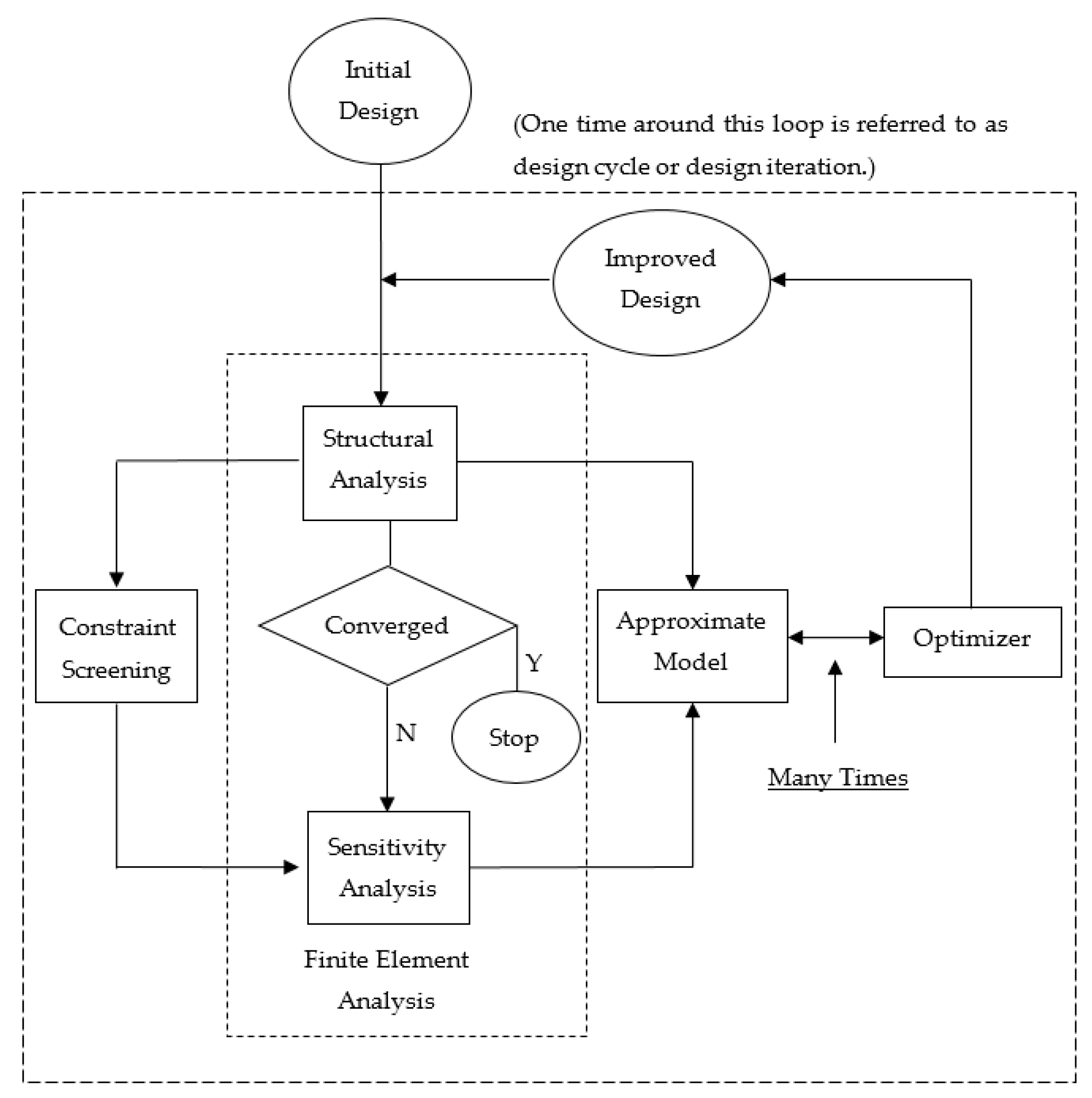
The MSC Nastran design optimization process is composed of finite element analysis, constraint screening, sensitivity analysis, approximate and improved models, and the optimizer. The optimization process is started with the finite element analysis of the initial design; subsequently, the analysis is repeated multiple times during the process, with the repetition frequency defined by the design sensitivity. Constraint screening is required to select constraints that may start the redesign process. Designs constraints near the violation threshold or that are already violated are activated during constraint screening. Design sensitivity analysis calculates the speed of change of the structural response and constraint values with changes in design variables. When design optimization is required, the sensitivity analysis function is called automatically. The finite element analysis results are approximated and combined with the information obtained during sensitivity analysis to form the approximate model. This approximation allows for minimizing the complex finite element analyses. The approximate model is used during the optimization process to construct the improved model. In MSC Nastran, gradient-based, sequential linear programming and sequential quadratic programming optimization methods are available to improve the approximate model. A soft convergence test is performed by comparison of approximate and improved models, and convergence is achieved when the changes to the model are within required range. If the design has not converged, another loop of the optimization process is initiated by finite element analysis of the improved model. A hard convergence test is performed by comparison of current and previous design cycle finite element analysis results. The design optimization loop may be interrupted when either hard or soft convergence is achieved. The structural optimization process can be significantly improved if certain approximation concepts are applied.
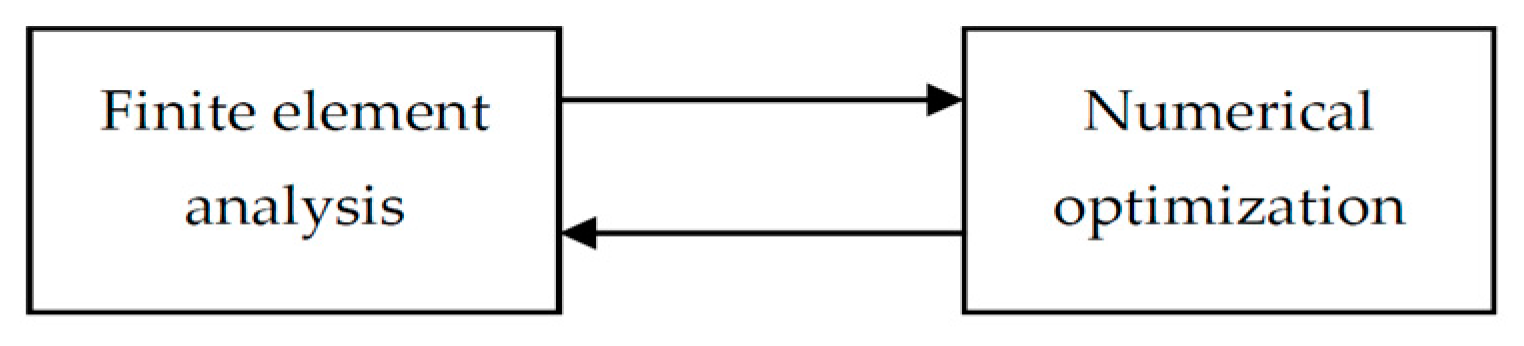
During the optimization process, numerous function evaluations and response derivations are required to compute design responses and sensitivities, respectively. Figure 1 illustrates the traditional approach to the structural optimization, where every request for function evaluation requires finite element analysis of the model. Since the finite element analysis needs a significant amount of computational power, the traditional approach can only be used to solve small-scale design problems.
To reduce the number of finite element analyses, approximation concepts have been developed and implemented in MSC Nastran. These concepts that can be classified as design variable linking, constraint screening and the approximate design model, are described below.
2.1. Design Variable Linking
In general, the design task can be narrowed if the number of design variables is minimized. To improve the efficiency of design optimization and reduce the amount of computation, proportionally transformed design variables should be combined together, resulting in a significantly reduced set of variables. Ideally, a small number of independent variables should be used during design optimization. In MSC Nastran, design variable linking is manually performed by the user. Other concepts, such as the screening of design variables, could be considered. Pre-screening for the dimensional reduction of designs and for variable selection could play an important role in reducing the cost of the design task by identifying the most important design variables; this would allow the user to deal with large-scale design optimization problems more effectively.
2.2. Constraint Linking
Constraint screening is another concept that can be applied to the design optimization process to reduce the required computational power. Only constraints that are near the violation threshold or are already violated should be considered during optimization, while non-critical design constraints can be deactivated. In other words, only those constraints that can trigger the redesign process should be visible to the optimizer. Constraint screening will also simplify sensitivity analysis by reducing the number of structural response derivatives required to compute design sensitivities. The reader may wish to refer to Appendix A.2 for some background information on the field.
2.3. Approximate Design Model
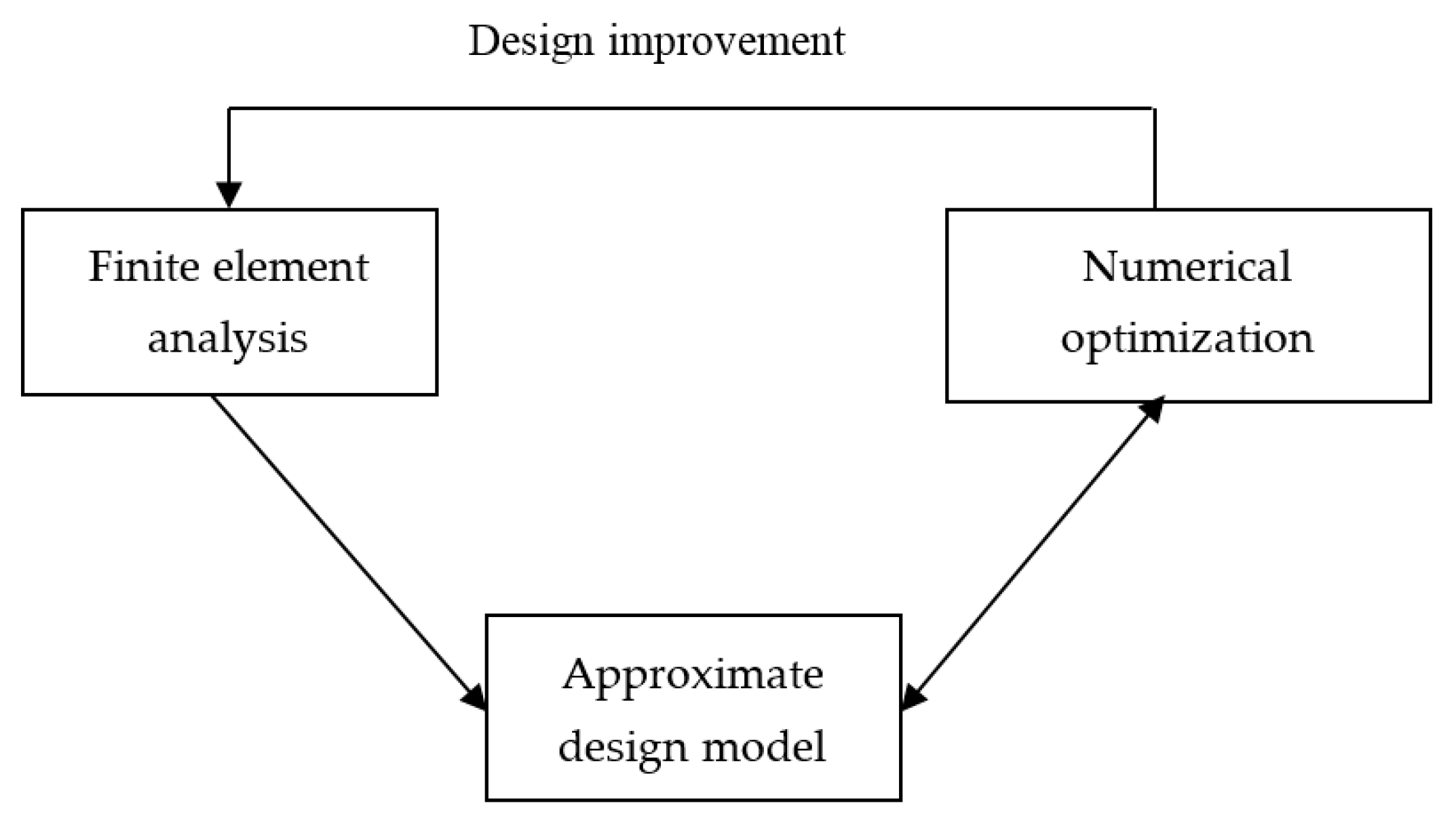
In order to establish how the active constraint set is affected by design modifications, parametric analysis is performed after the constraint screening. Response quantities, used in a parametric analysis, are approximated or expanded in series in terms of design variables. Compared to implicit finite element analysis results, formal approximations are explicitly expressed in design variables. Explicit formal approximations, computed using sensitivity analysis results, are used by the optimizer during gradient or function evaluations. Figure 2 shows how the approximate design model is created and evolves during the optimization process. The approximate model involves the construction of high-quality approximations to the finite element results, so that the number of full-scale finite element analyses can be kept to a minimum. The core of the approximate model is formed by formal approximation of the finite element analysis results. Constraint screening and design variable linking are used to simplify the approximate model. It should be noted that in MSC Nastran, formal approximation and constraint screening are automated [27]. The approximation functions used are based on Taylor series expansions of the objective function and constraints. Given a function , an infinite series about a known value in terms of the change in an independent variable can be written as
In addition to the function value , this series requires that all derivatives at be known as well. Determining these derivatives may present some difficulty, so the series is often truncated to a given power in , yielding an approximate representation of the original function. In the design optimization process, where we are concerned with a vector of design variables , the approximations for the objective function and the constraints become
where a gradient term replaces the first derivative term of Equation (1).
When the new configuration is generated by the optimizer, the proposed design is analyzed to ensure that the design constraints are satisfied and the objective function has been improved. This process is illustrated by the ‘design improvement’ arrow in Figure 2. If further design optimization is required, the finite element analysis is performed again to form the basis for the next generation approximate model. The sequence of design modifications, also referred to as design cycles, may be repeated a number of times. Design convergence is achieved when another design cycle or the optimizer are unable to produce significant changes to the model. The detailed schematic diagram of MSC Nastran design cycle is illustrated in Figure 3 [27]. Compared to the traditional design approach where the finite element model is optimized, MSC Nastran operates with the approximate model. When the updated design configuration is generated, a finite element analysis creates new version of the finite element model based on the results produced by the optimizer.
3. Formulation of the Structural Optimization Problem
Structural optimization problems are characterized by the nature of the objective and constraint functions, which are generally nonlinear functions of the design variables. Usually, these functions are non-convex, discontinuous, and implicit, as in many problems in engineering design. Furthermore, due to manufacturing constraints, design variables are quite often restricted to taking discrete values from a set of standard sizes, which gives rise to mixed integer nonlinear optimization. Mathematically, the optimization problem can be described as minimizing or maximizing the objective function with respect to the design variables x under the inequality constraint and the equality constraint . The structural optimization problem can be formalized and written as follows:
Here, is the scalar objective function, is the vector of n components, is the vector of inequality constraints, is the vector of equality constraints, and are the lower and upper bounds on each of the design variables (design search space), respectively, is the vector of discrete design variables, and is the set of discrete values. The inequality and equality constraints and demand a solution x to be achievable only if all the constraints are satisfied. The set of all feasible solutions is named the feasible space. Typically, at least one solution x exists in the feasible space, and if this solution corresponds to the minimum objective value it is called the optimum solution.
4. Gradient-Based Optimization Solution Procedure
Gradient-based algorithms use function gradient information to search for an optimal design. The first step in the numerical search process is to calculate the gradients of the objective function and the constraints for a given point in the design space. The gradients are calculated using a first-forward finite difference approximation of the derivative (finite difference techniques). Appendix A.1 provides the reader with more details. Once the gradient is computed, there are several options for finding a minimum. For constrained problems, sequential quadratic methods and the Modified Method of Feasible Directions (MMFD) can be used [28], whereas for unconstrained problems, quasi-Newton methods are effectively used with a line search procedure [29]. As the search direction is determined, the search process continues in that direction and can be repeated until an optimum solution has been found. The choice of optimization method and solver is design-dependent, and generally the size of the problem and the accuracy and precession of the solvers play an important role in making the decision. In this study, the commercially available off-the-shelf MSC Nastran software is used. The design optimization module is based on gradient-based solution techniques. It utilizes the MMFD of Design Optimization Tool (DOT) and MSCADS, a modified version of the Automated Design Synthesis (ADS) code for performing size optimization.
4.1. Generating Good Initial Points for the Design
Since gradient-based optimization methods do not guarantee global optimality, different approaches are used to enhance the performance of the optimization design models by generating good initial starting points for the design variables. In the first approach, two essential starting points are assigned by the user as initial starting points. Typically, the upper and lower bounds of the continuous or discrete design variable are used. A number of interior points in the bounded design region are chosen by the user as additional initial starting points to cover more regions in the design space. These interior points can be randomly selected in the design space or, more practically, can be defined as a fraction of the upper bound value of the design variables, or by using the internal halving method. Given a bounded design space , where the bounds on each of the design variables are in the form , a set of initial starting points {, , , , ..., } is generated, where , and R {, , , ..., }. is a set of additional interior points which can be generated using one of the following methods:
- As a fraction of the upper bound value of the design variables:where is a fraction value defined by the user between , with
- Internal Halving Method:
In both methods, the interior points selected must be reasonably separate from each other to minimize the number of repeated visits to the same region of attraction in the search design space, and to avoid the optimizer getting stuck in local optima where no improving neighbors are available. In the second approach, the Fully Stressed Design (FSD) algorithm, which is widely applied in the design of structures, is used to produce an initial design from a set of different starting points for the design variables provided by the user at the start of the optimization process. Even within the limited class of problems that can be addressed, and its capability of handling a design condition subjected to strength limits only, the FSD algorithm can still provide an efficient way to begin a design task, and the output can still serve as an excellent starting point for more general optimization tasks that need to satisfy a variety of design criteria. The FSD provides a quantitative value for the best-case estimate on the amount of material required to satisfy the applied design conditions. This technique is particularly useful if the structural weight minimization of the designed aerospace construction is the most important requirement. This method is basically useful for the design of aerospace structures where the overriding requirement is that the structural weight be minimized. The basic concept of the FSD algorithm is summarized in [27].
4.2. Practical Optimization Framework
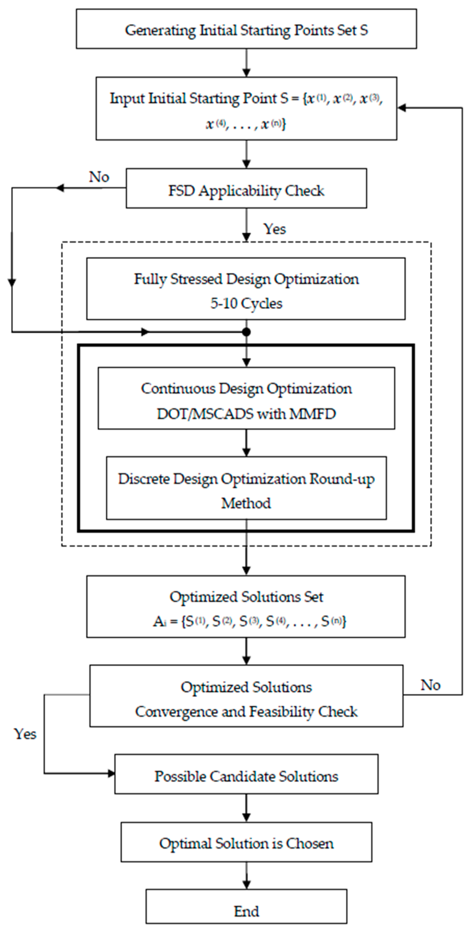
Gradient-based algorithms are very efficient at operating local searches but not so good at global searches, due to their tendency to get stuck in local optima and thus not make a thorough exploration of the design search space. A practical optimization framework is presented in this study to enhance the overall performance of the optimization gradient-based algorithms. The first step is to generate a set S of initial starting points for the design variables. Then, we must decide on the number of starting points to try and how to distribute them in the search design space. This decision is usually guided by intuition and previous experience, since there is no clear methodology available as a guide. The applicability of the FSD procedure is checked by the structural designer. If it is applicable, then a number of FSD cycles, usually 5–10 cycles, are used to generate a solution based on the FSD concept that will hopefully serve as an improved starting point for the optimization process, because optimization can give very poor results if poor initial guesses for the design variables are used. More general optimization algorithms are used in the later steps of the optimization process. The idea here is to use two different gradient-based algorithms rather than just one. The reason behind this approach is the fact that the two different algorithms will likely have completely different search directions between the initial and final points, which are output as the solutions. The DOT and MSCADS optimization codes implemented in MSC Nastran with the MMFD are used to perform continuous and discrete optimization. Discrete optimization in MSC Nastran is implemented as a post-processing step to a continuous solution or FSD; this means one additional finite element analysis followed by the discrete optimization results. As a result, a set of solutions called Ai is created. This set contains all optimized solutions obtained using the set S of the initial starting points. Each solution is then checked to see if it meets the convergence criteria and if it is a feasible design. If this is the case, the solution with the minimum optimized mass that satisfies all the design requirements is chosen as the best of all possible candidate solutions. On the other hand, if no feasible solution exists, the user can try to test different sets of initial starting points, making sure that the optimization problem is a well-conditioned one, that no errors have been made in specifying the model constraints, and that no wrong numbers in the data are used in the optimization. This process can be repeated until all the initial starting points defined by the user are exhausted or when the computational resources used by the algorithms, such as the computation time and memory space, exceed pre-defined limits. Figure 4 shows a flowchart of the proposed practical framework.
4.3. Improving the Search for the Optimum Solution
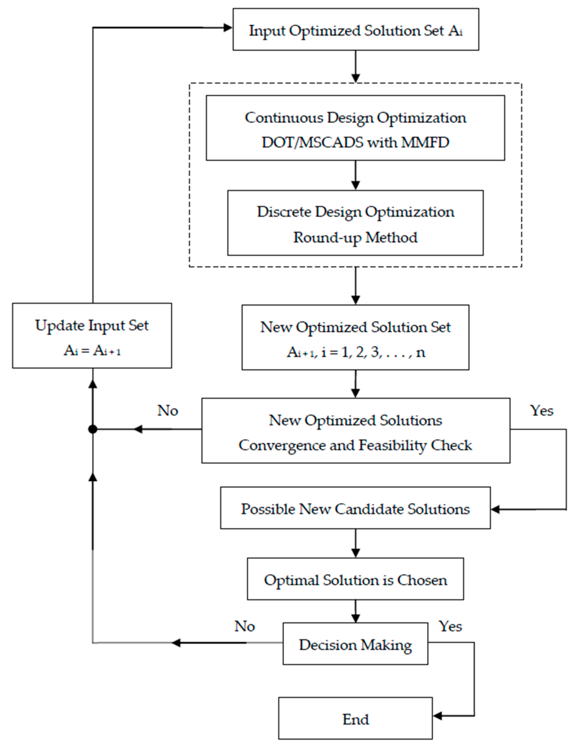
In practice, difficulties can emerge when trying to solve a structural optimization problem, especially when the design space is too large and contains design variables of different sensitivities, or when the optimization problem has highly nonlinear objective and constraint functions. Problems also occur when the design variables are discrete, meaning that the search design space is discrete too. In such scenarios, it can be difficult to achieve a convergence solution, leading to a final design that is unfeasible [30]. In this study, an improved strategy is proposed and used to enhance the search for the optimum solution. Figure 5 shows a flowchart of this improved strategy.
The strategy employed in the present work is to take the design solutions obtained using one algorithm and use them as a starting point for the other one and vice versa. A continuous and discrete optimization solution is performed and a new set of solutions, Ai + 1, is obtained at the end of the process. Convergence and design feasibility checks are performed, as explained in the previous section, and the solution with the minimum optimized mass that satisfies all design requirements is chosen as the best of all possible candidate solutions. In the same manner, the proposed strategy can be used to search for an improved optimum solution from the one obtained using the framework described in the previous section. This process can be repeated until an optimum feasible solution is obtained, or an improvement in the values of the design objective is achieved.
5. Structural Design Optimization Case Studies
The public domain NASA wing, commonly referred as Common Research Model (CRM), is used as a design and optimization case study [31,32] to demonstrate the efficiency and reliability of the proposed practical optimization framework and improved strategy. The relevant aircraft data are presented in Table 1.
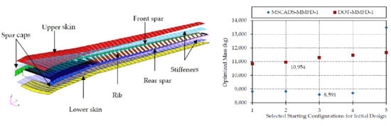
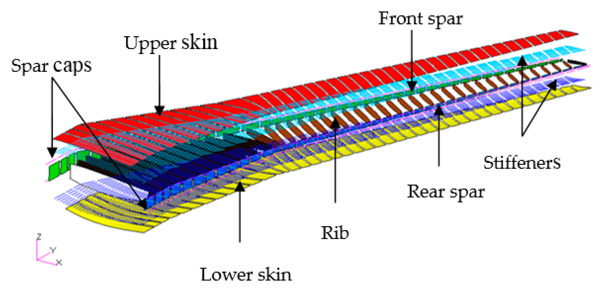
The CRM wing considered in the case studies is modified to have airfoil sections with the same twist angle along the semi-span of the wing. Therefore, the chord lines of the airfoils at the root and tip wing sections are rotated in a spanwise direction with respect to the chord line of the airfoil at the kink wing section to produce a similar geometrical twist angle of 0.8°. The CRM primary wing structure is modeled to meet the minimum design requirements set forth by the Federal Aviation Regulations (FAR) Part 25 [33] and/or the European Aviation Safety Agency (EASA) CS-25 [34]. A traditional two-spar wingbox architecture is used as a baseline design. The external geometry is defined by CRM.65-BTE airfoil sections and the wingbox is derived from the wing surface model by defining the front and rear spar positions at 12% and 71%, respectively, of the local airfoil chord. The internal layout is defined by the stiffener pitch, rib pitch, and orientation based on the values for a typical large transport aircraft wing. The wingbox model contains 1870 design zones for the upper and lower skins, spar webs, ribs, spar caps and stiffeners, as given in Figure 6. The chordwise design zones are prescribed by the stiffener pitch, while in the spanwise direction the design zones are limited by the rib spacing. In the finite element model, each design field consists of a number of finite elements that all comprise the same thicknesses/cross-sectional areas and stiffness properties.
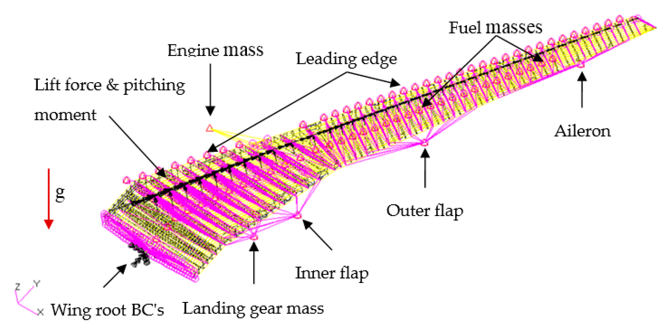
In the current study, the thin-walled structures of the CRM wingbox configurations (skins, webs and ribs) were modeled using two-dimensional quadrilateral and triangular shell elements (CQUAD4, CTRAI3) with in-plane membranes and bending stiffness. On the other hand, stiffeners and spar caps were modeled using one-dimensional rod elements (CROD) with axial stiffness. The CRM aircraft wingbox is optimized subjected to aerodynamic loads, lift force, and pitching moment, with inertial relief loading due to the engine, fuel, and undercarriage masses as well as the mass of the wingbox itself and the secondary structure masses, as shown in Figure 7.
The 2.5 g symmetric pull-up maneuver load is considered as critical for the design, analysis, and sizing optimization of the CRM wingbox. In the current study, the aerodynamic loads are calculated with two different programs in order to ensure the versatility and accuracy of the tool. Two existing aerodynamic codes are used for this work, including the ESDU 95010 computer program [35] and the Tornado VLM code [36] implemented in MATLAB. Aerodynamic loading is discretely distributed along the wing by computing the equivalent lift force and pitching moment components at rib boundary locations at 25% of the local chord length. The aerodynamic loads are introduced to the wingbox structure by means of multipoint constraint (MPC) non-stiffening rigid body elements (RBE3) in the rib’s perimeter nodes. The engine mass is modeled as a concentrated lumped mass using point elements at the centre of gravity of the engine. For the engine pylon, a simple beam structure was created to realize a distributed engine pylon-to-wingbox connection. Rod elements (CROD), mounted on front and aft fittings, modeled using a combination of non-stiffening (RBE3), and stiffening (RBE2) rigid body load carrying elements, are used to model the engine and pylon structural components. Due to the high complexity level of the geometrical and structural modeling of the main landing gear, its component masses are modeled as a concentrated lumped mass using point elements, and it is introduced to the wingbox structure rear spar at its centre of gravity position using RBE3 elements. The component masses of the leading and trailing edge devices are estimated based on the corresponding surface area using the semi-empirical and analytical equations of Torenbeek [37]. The inertial load impacts of these masses are modeled as lumped masses using point elements at the centre of area of the leading and trailing edge devices, and are attached to the front and rear spars of the wingbox along the span via RBE3 interpolation elements. The inertial load impact of the wingbox self-structural mass is derived by adding a downward gravitational acceleration (g = 9.81 m/s2) to the finite element model of the wingbox. Spring elements (CEALS1) combined with RBE2 elements are used to create realistic boundary conditions at the wingbox root at the aircraft centerline. The translational and rotational stiffness properties were selected to result in end boundary conditions sufficiently close to the clamped case.
5.1. Definition of the CRM Wingbox Optimization Problem
The CRM wingbox structural optimization that is presented in this study purposely deals with property optimization. Therefore, the locations of the ribs, stiffeners, and spars are considered invariable and shape optimization is not performed in this study. The aim of the study is to minimize the masses of the metallic and composite configurations of the CRM wingbox when subjected to static strength/stiffness constraints and side constraints (manufacturing requirements) on the design variables. The optimization problem is mathematically formulated in this section as previously described in Section 3. The objective function, static strength/stiffness constraints, side constraints, and the types of design variables involved in the optimization problem are identified.
5.1.1. Objective Function
The objective function is the structural mass of the CRM wingbox excluding any non-structural masses, like fuel mass, landing gear mass, and engine mass. The objective function can be represented by:
5.1.2. Design Variables
For the optimization problem, considering the wingbox construction material to be a metallic material, one design variable per design field is defined. The design variables include the thicknesses of the wingbox skins, spar webs, and ribs, as well as the cross-sectional areas of the wingbox spar caps and stiffeners. A minimum gauge thickness of 2 mm and a cross-sectional area of 144 mm2 are specified for the design variables. The limits on the design variables are defined as follows:
On the other hand, considering the wingbox construction material to be a composite material, the corresponding design variables for the wingbox skins, spar webs, and ribs are the thicknesses of each ply or lamina in the composite laminate associated with each design field. The cross-sectional areas of the composite spar caps and stiffeners are also treated as individual design variables for each design zone. For modeling the wingbox using a composite material, a symmetric and balanced laminate with ply orientation angles of [45/0/–45/90]s is created to obtain an orthotropic material. The minimum ply thickness is taken to be 0.127 mm, while a 3 mm minimum gauge laminate thickness is recommended to maintain an adequate level of laminate damage tolerance. The laminate ply thicknesses are treated as individual design variables and a count is made of the required number of plies in each ply orientation angle. The limits on the number of plies in each ply orientation angle are given as
Minimum cross-sectional areas of 216 mm2 for the composite spar caps and stiffeners are specified and the limits on the design variables are defined as
5.1.3. Static Strength Constraints
The failure mode of the wingbox structural components depends on their allowable stress/strain state based on the load case under consideration and the construction material. Thus, for the metallic CRM wingbox structural elements (skins, spar webs, ribs, and spar caps/stiffeners), the strength constraints imposed in each design zone can be described as follows. For metallic skin panels, spar webs, and ribs, the von Mises stress is checked against the material allowable stress as defined in the following equation:
The allowable limit value is obtained by dividing the ultimate stress by a factor of 1.5. The von Mises stress criterion is useful since it is a single equation and is accurate for ductile materials such as aluminum alloys, which are widely used in the construction of aircraft structures. The metallic spar caps and the longitudinal stiffeners are designed to carry axial stress only. Therefore, they are designed according to their stress state (tension or compression) against the allowable stress of the material as defined in the following equation:
For composite skin panels, spar webs and ribs, the Tsai–Wu criterion [38,39,40] is used to predict the strength of the composite laminate in terms of the failure index (). For orthotropic plate analysis, under the plane stress state, the Tsai–Wu strength theory predicts that a lamina will undergo failure when the following inequality is satisfied:
The coefficients –, with the exception of , are described in terms of strengths in the principal material directions. accounts for the interaction between normal stresses, and .
The principal strains in each ply are also checked against the material allowable strain to ensure the integrity of the plies and failure-free laminates. Thus, the following constraint is placed on the strain value used for sizing the structure:
The ultimate strain value to be used is suggested in [41] to be 0.5%, and the allowable limit value is obtained by dividing the ultimate strain by a factor of 1.5. The allowable strain value of 0.35% (3500 με) includes the margins due to fatigue and damage tolerance, assuming that the allowable strains are identical in terms of tension and compression. The composite spar caps and longitudinal stiffeners are designed to carry axial stress only. Due to the orientation of the fibers in the longitudinal direction of the composite rods, the longitudinal strength of the composite rods is considered to be much higher than the transverse strength. Longitudinal properties are dominated by the fibers, while the transverse properties are dominated by the matrix. Therefore, the composite rods are designed according to their stress state (tension or compression) against the allowable stress of the longitudinal fibers. Generally, to obtain the properties of the composite rod, rod samples are tested for compression and tension. However, in this study, the assumed allowable stress value has been obtained by dividing the stress of the longitudinal fibers by a factor of 2. The use of a factor of safety greater than 1.5 is recommended for composite rod analysis, to account for the possible uncertainty and variability of the values of the rod properties. The axial stress constraint can be written as
5.1.4. Static Stiffness Constraints
In aircraft wing design, a major requirement for stiffness arises from diverse considerations such as aeroelasticity, wing flexibility and redistribution of aerodynamic loads and these effects may be included in the optimization process. Torsional stiffness is necessary to counteract the twisting of the wing under aerodynamic loads and thus prevent flutter. The flexibility of the wing can cause undesirable effects on its aerodynamic performance. Lift loss due to wing deformation is one of these effects that must be taken into account in the aerodynamic load calculation. The change in wing twist distribution and bending under aerodynamic loads can have a significant effect on the wing incidence angle and consequently the aerodynamic loads acting on the wing. The redistribution of aerodynamic loads results in the redistribution of stresses/strains in the wing structures, and as a result failure can occur. Therefore, the flexural stiffness of the wingbox is controlled by limiting the vertical displacement of the wingtip leading edge, and the torsional stiffness is controlled by constraining the twist angle at the tip chord of the wing.
In general, structural stiffness information is not publicly available for commercial aircraft. However, some estimation can be made on the structural stiffness of the wingbox, providing the wing deflection is known. In this study, the wingtip deflection for the CRM wing at a 2.5 g pull-up maneuver is assumed to be 15% of the wing semi-span b. This is based on the relative deformations that can be expected in the wing of a transport-category aircraft as a function of the load factor, as presented in the open scientific literature [19,42]. This value also ensures that the aircraft wingtip does not strike the ground during a taxi bump load or landing operation. The current maximum allowable deflection constraint placed on a single component of the displacement at a prescribed node is defined as follows:
The angular deformation at the wingtip chord is constrained by limiting it to a value of 6° to ensure sufficient torsional stiffness and thus an adequate aeroelastic response [43]. The twist angle constraint is defined using the vertical displacements at the wingtip chord ends. Equation (18) shows that the twist angle at the wingtip should not exceed 6°. and are the maximum vertical displacements in positive and negative directions of the z-coordinate, respectively. Here, is the wing chord length at the required location:
5.1.5. Static Stiffness Constraints
Practical design rules and manufacturing constraints are considered during the design and optimization process of the CRM wingbox. A minimum gauge thickness of 2 mm is considered for the design of the metallic wingbox thin panel structures. This is because the value of 2 mm is considered an acceptable sheet metal thickness if rivets are to be used as mechanical fasteners to join the sheet metal parts of the aircraft together. For ease of manufacturing, the thin panel thicknesses of the wingbox are chosen from a set of discrete values defined between the lower bound and the upper bound and incremented by 0.1 as
Generally, the calculation of the cross-sectional areas of the spar caps and stiffeners depends on the shape and dimensions of the cross-section of a given profile. In this study, the metallic and composite spar caps and stiffeners are modeled using rod elements, and therefore for ease of manufacturing the rods are sized using a discrete set of values from which any flange shape, such as L, T, and Z shapes, can be produced. The discrete sets of cross-sectional areas for the metallic and composite rod elements are defined as
For ease of manufacturing, the limits on the number of plies in each ply orientation angle are selected from a set of discrete integer values defined between the lower bound and the upper bound and incremented by 1 as
Practical design criteria are applied to the design and optimization process of the composite laminate wingbox structures. The ply orientation percentages within a laminate are bounded by lower and upper bound values of 10% and 60%, respectively. This aims to avoid matrix-dominated behaviors. An optimization constraint is applied to link the +45° and −45° layers, ensuring that their thicknesses are identical. This is done to ensure that the laminate is balanced and to minimize the possibility of introducing manufacturing stresses such as torsion. A maximum property drop-off rate criterion is applied. It aims on the one hand at avoiding delamination and, on the other hand, at obtaining ply layouts that can actually be manufactured. The property drop-off rate between neighboring elements/panels is evaluated according to the following equation [44]:
where is the element/panel property value of the parent (1) or adjacent (2) element/panel, and the distance is computed along the element/panel surfaces between adjacent centroids.
5.2. CRM Wingbox Case Studies
The CRM wingbox considered in this case study is optimized to meet static strength and stiffness requirements and manufacturing constraints. Five different initial starting point values are used for the design variables during the optimization process. MSC Nastran Sol 200 is used for the sizing optimization of the wingbox model. A number of fully stressed design cycles are performed at the beginning of the optimization process, followed by a number of continuous and discrete optimization cycles. Both optimization algorithms, DOT and MSCADS, are individually used to solve the optimization problem. Then the estimated solution is updated on an iteration-by-iteration basis with the aim of improving the optimum value of the mass of the CRM wingbox model.
5.2.1. Metallic Wingbox Model
In this case study, the wingbox of the CRM aircraft is designed by considering metallic materials with a total number of 1870 design variables. High-strength aluminum 7050-T7451 alloy [45] is used for the design of the upper skins, upper stiffeners and spar caps, and 2024-T351 alloy [46] is used for the design of the lower skins, lower stiffeners and the ribs, since it is better suited for structures stressed by cyclic tension loads and therefore prone to fatigue damage. The physical and mechanical material properties are listed in Table 2.
Table 3 shows the optimized masses of the metallic CRM wingbox using different starting values for the design variables defined as fraction of the upper bound value of the design variables along with different optimization algorithms. In all solutions, convergence is achieved along with feasible discrete designs. The bold value denotes the local minimum solution obtained.
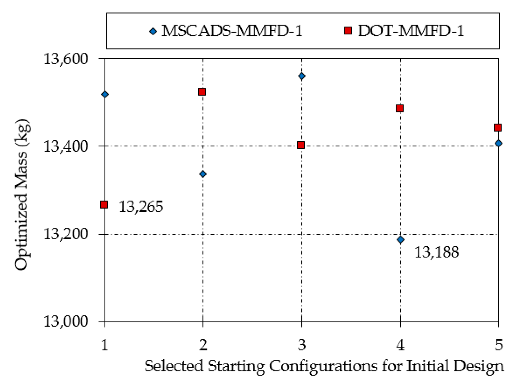
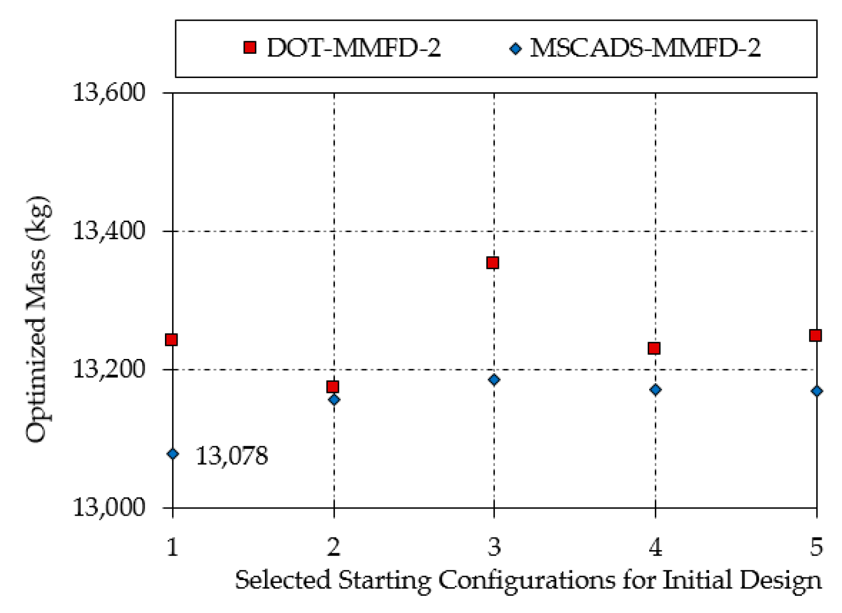
Figure 8 and Figure 9 illustrate the results of the first and second optimization iterations obtained using the DOT and MSCADS algorithms for the metallic CRM wingbox model.
From the results presented in Table 2 and illustrated in Figure 8 and Figure 9, the following observations can be made. In the gradient-based optimization problem, using different starting values for the design variables can lead to local optimum designs, since the optimized wingbox configurations do not have exactly the same mass. Similarly, different gradient-based algorithms used to perform the same optimization problem terminate at different local optima, and thus return different solutions even for the same initial starting values for the design variables. It is also observed that optimum solutions are not restricted to extreme or corner points of the research design space. Furthermore, it can be seen that the minimum optimized mass of the metallic CRM wingbox is obtained using the MSCADS-MMFD-2 iterative solution with a value of 13,078 kg. Comparing this value with the related optimized value (13,265 kg) obtained earlier in the first iterative solution, and with the minimum optimized value (13,188 kg) obtained using MSCADS-MMFD-1, it can be seen that the value of the objective function against the initial optimized value has improved.
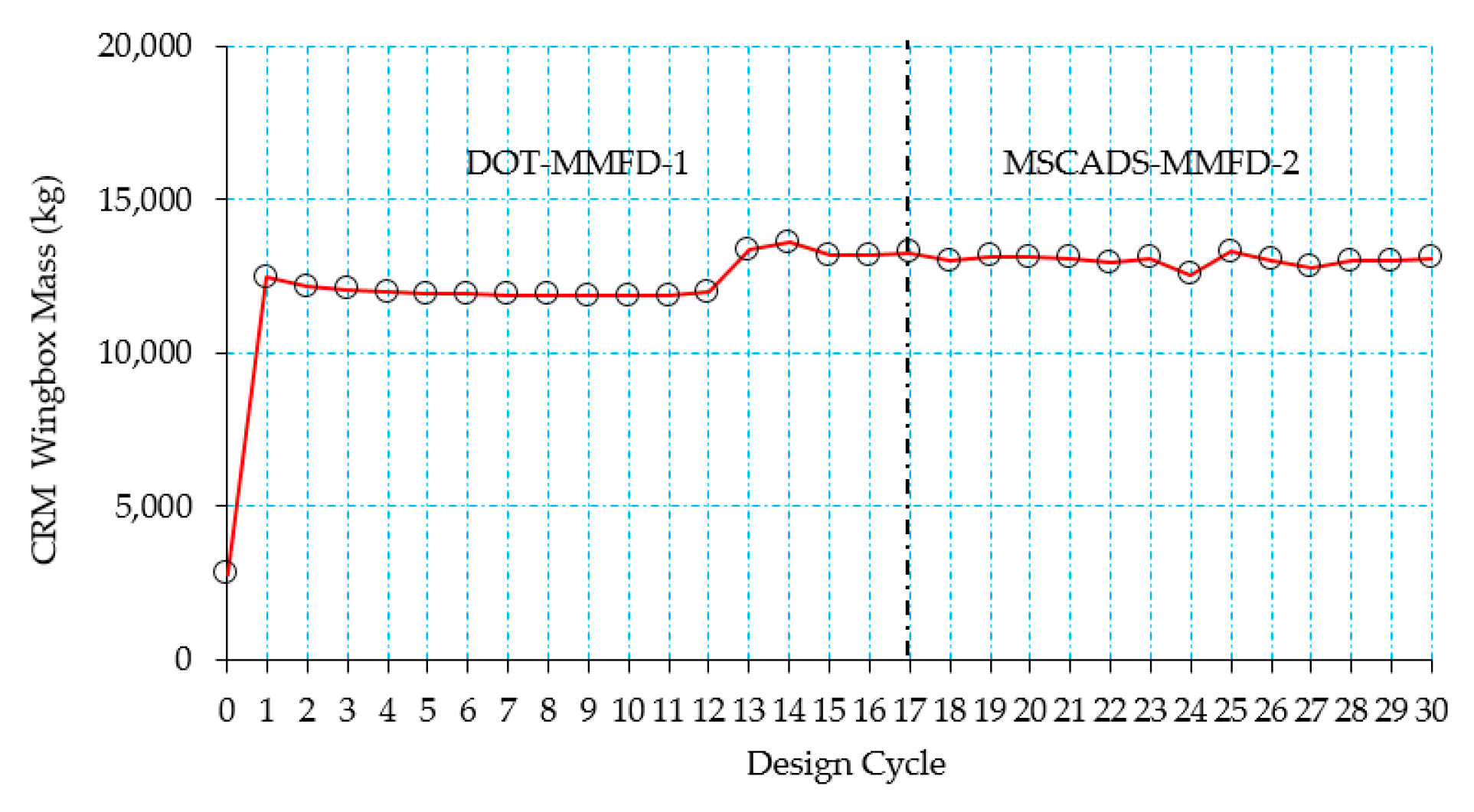
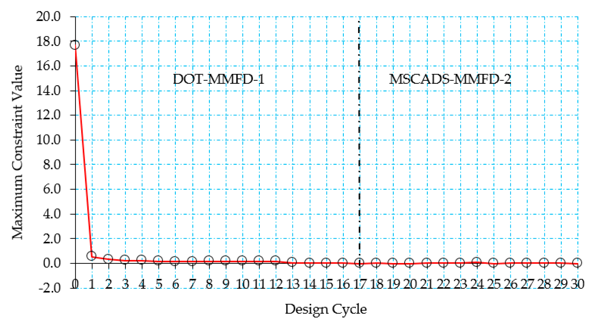
Figure 10 shows the history of the objective function as a function of the design cycles for the metallic CRM wingbox model. As can be seen from Figure 10, hard convergence to an optimum and feasible discrete solution is achieved in 17 design cycles for the metallic CRM wingbox using the DOT-MMFD-1 solution and an improved solution is founded using the MSCADS-MMFD-2 solution in 13 design cycles. The 0th design cycle corresponds to the initial mass of the wingbox model, which is based on the starting values of the design variables. Continuous optimization for the metallic wingbox model is achieved in 16 design iterations using the DOT-MMFD-1 and in 12 design iterations using the MSCADS-MMFD-2 solution. The 17th and 30th design cycles, as shown in Figure 10, correspond to the rounded-up discrete solution. In the round-up method, the standard size list for the design variables is used as a metric to round up continuous solutions for the design variables. Consequently, the increase of objective function value over the last design cycle in Figure 10 corresponds to the discrete feasible solution, founded by using the round-up method.
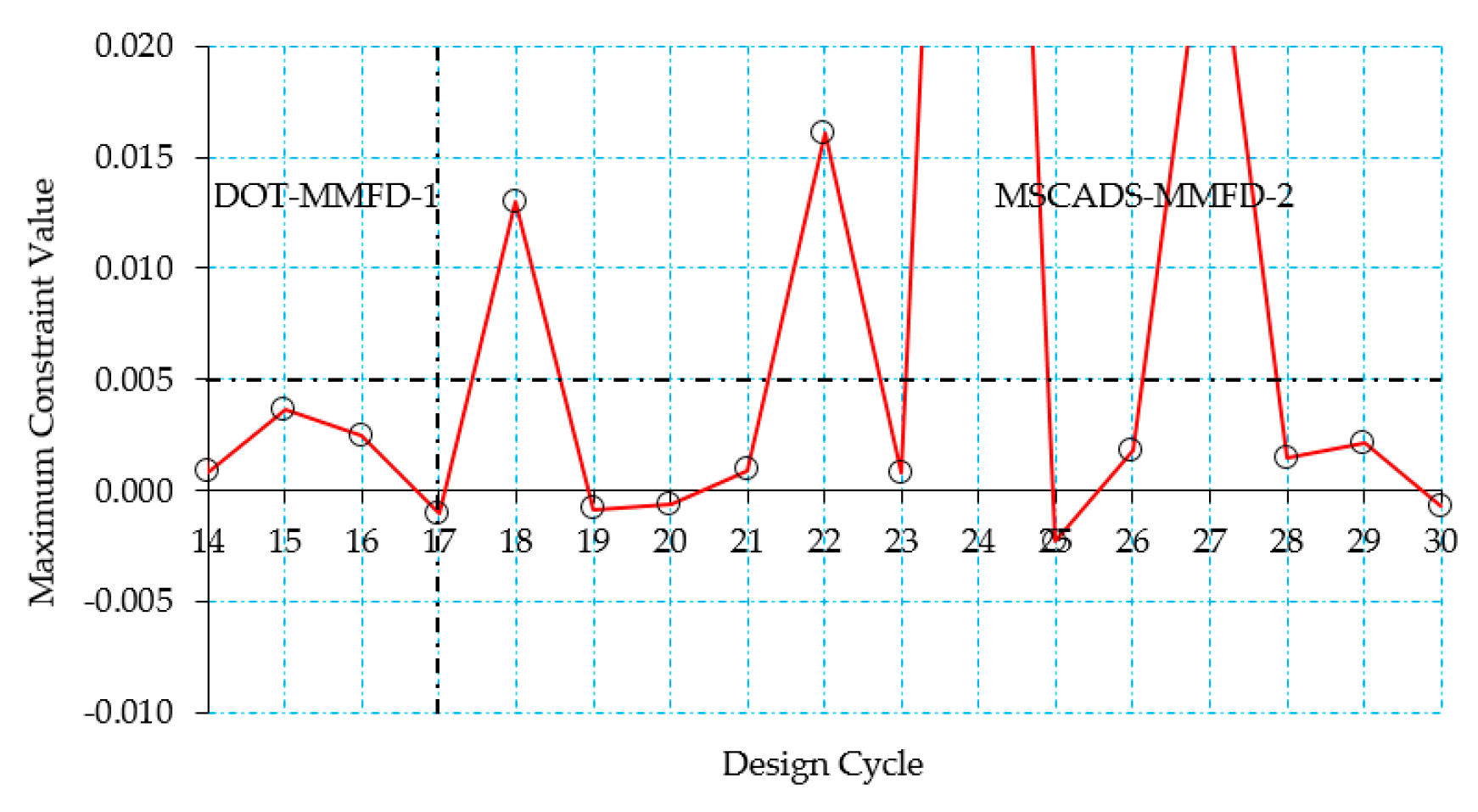
Figure 11 and Figure 12 (zoomed region) show the history of the maximum constraint value as a function of the design cycles for the metallic CRM wingbox model. As can be seen from Figure 11, the initial constraints are violated because the maximum constraint value is far greater than the allowable value of 0.005. The 0th design cycle corresponds to the initial mass of the wingbox, which is calculated using the lower bound of the design variables. In this case, the search direction has been chosen to reduce the constraint violation. Thus, the objective function value will increase, since the first priority is to overcome the constraint violations. If it is not possible to overcome the constraint violations in this direction, they may at least be reduced. By using a number of fully stressed design cycles at the beginning of the optimization process, the large value of the maximum constraint violation is reduced to a smaller value during the 12th design cycle, as can be seen from Figure 11. After this happens, the value of the objective function starts to increase, allowing additional reduction in the allowable constraint value as can be seen from Figure 10 and Figure 11.
5.2.2. Composite Wingbox Model
In this case study, composite materials made up of T300 carbon fibres and N5208 epoxy resin (widely used in the aircraft industry), are used as a second material choice for the design of the CRM wingbox structure with a total number of 2500 design variables. Table 4 defines the material properties of T300/N5208 [47].
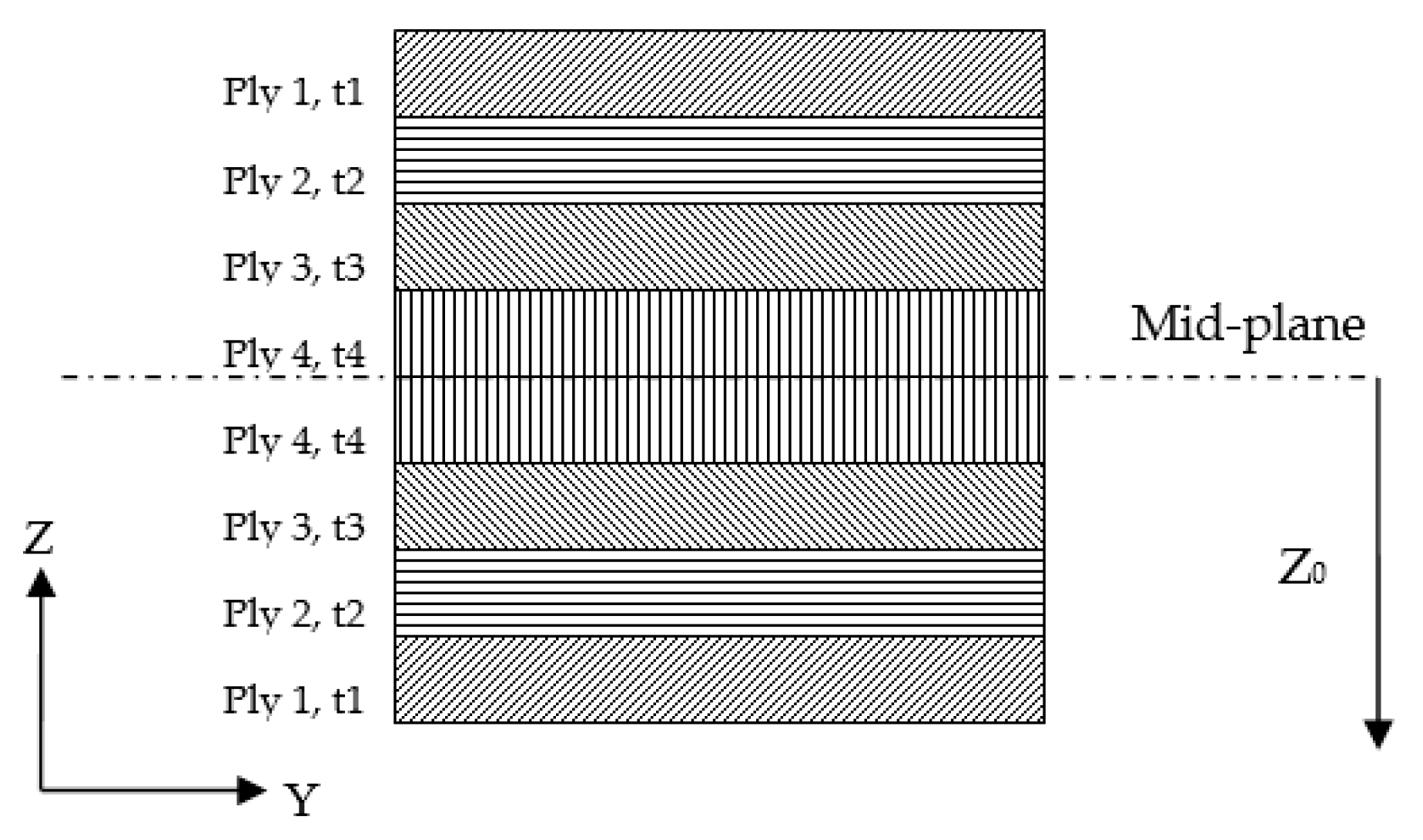
For modeling the wingbox using a composite material, a symmetric and balanced laminate with ply orientation angles of [45/0/–45/90]s was created in order to get an orthotropic material. The aim of this design procedure is to avoid shear extension and membrane bending coupled behaviors. The schematic of the composite laminate is given in Figure 13. The stacking sequence is symmetric about the mid-plane and is balanced with the same number of +45° and −45° plies. No 0° ply was placed on the lower or upper surface of the laminate. The minimum ply thickness is taken to be 0.127 mm; while a 3 mm minimum gauge laminate thickness is recommended to maintain an adequate level of laminate damage tolerance. The mechanical properties of the composite laminate were evaluated using the MSC Patran Laminate Modeler [48].
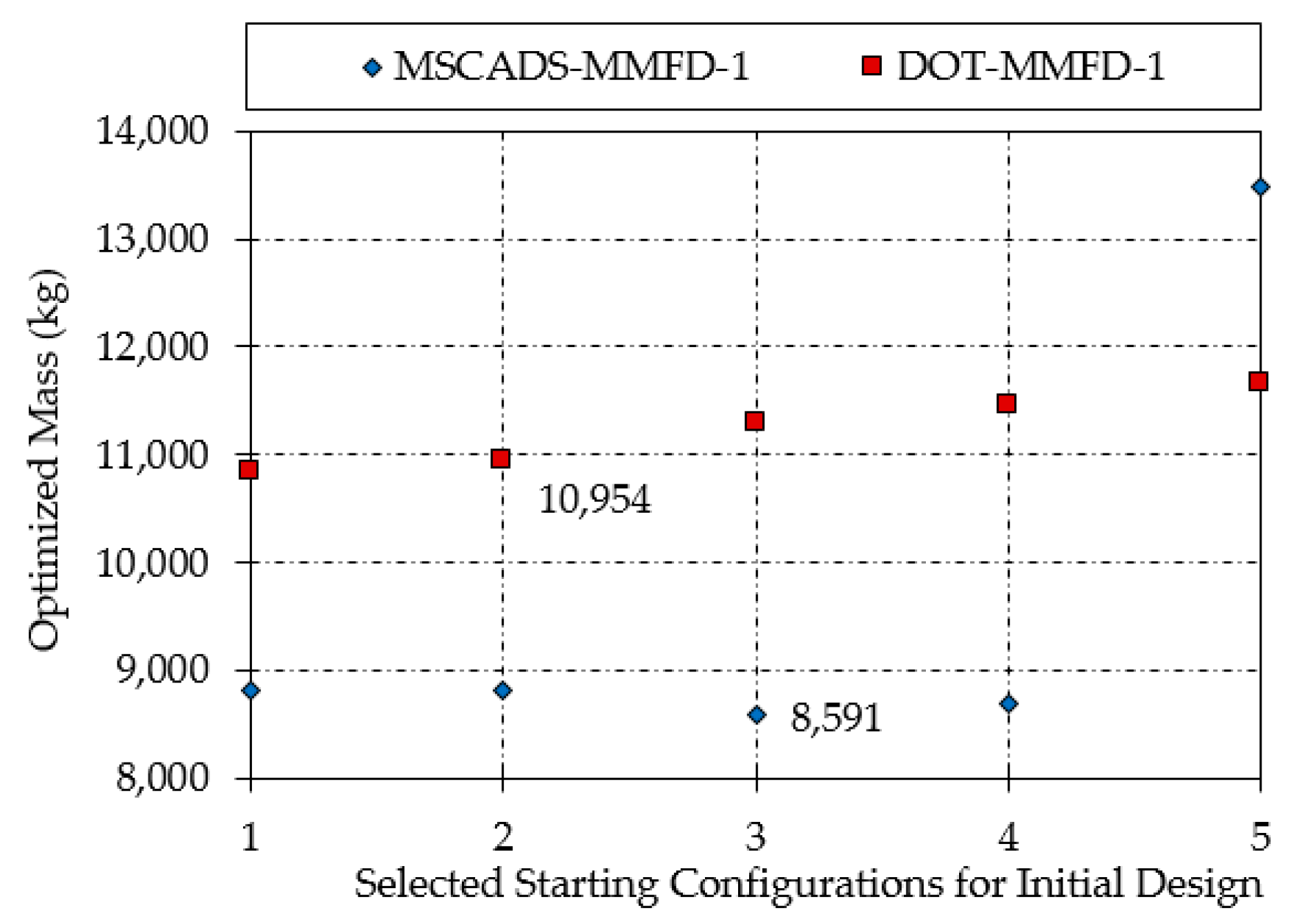
Table 5 shows the optimized masses of the composite CRM wingbox, using different starting values for the design variables along with different optimization algorithms. The bold values refer to the discrete feasible solutions that have been obtained for the composite CRM wingbox.
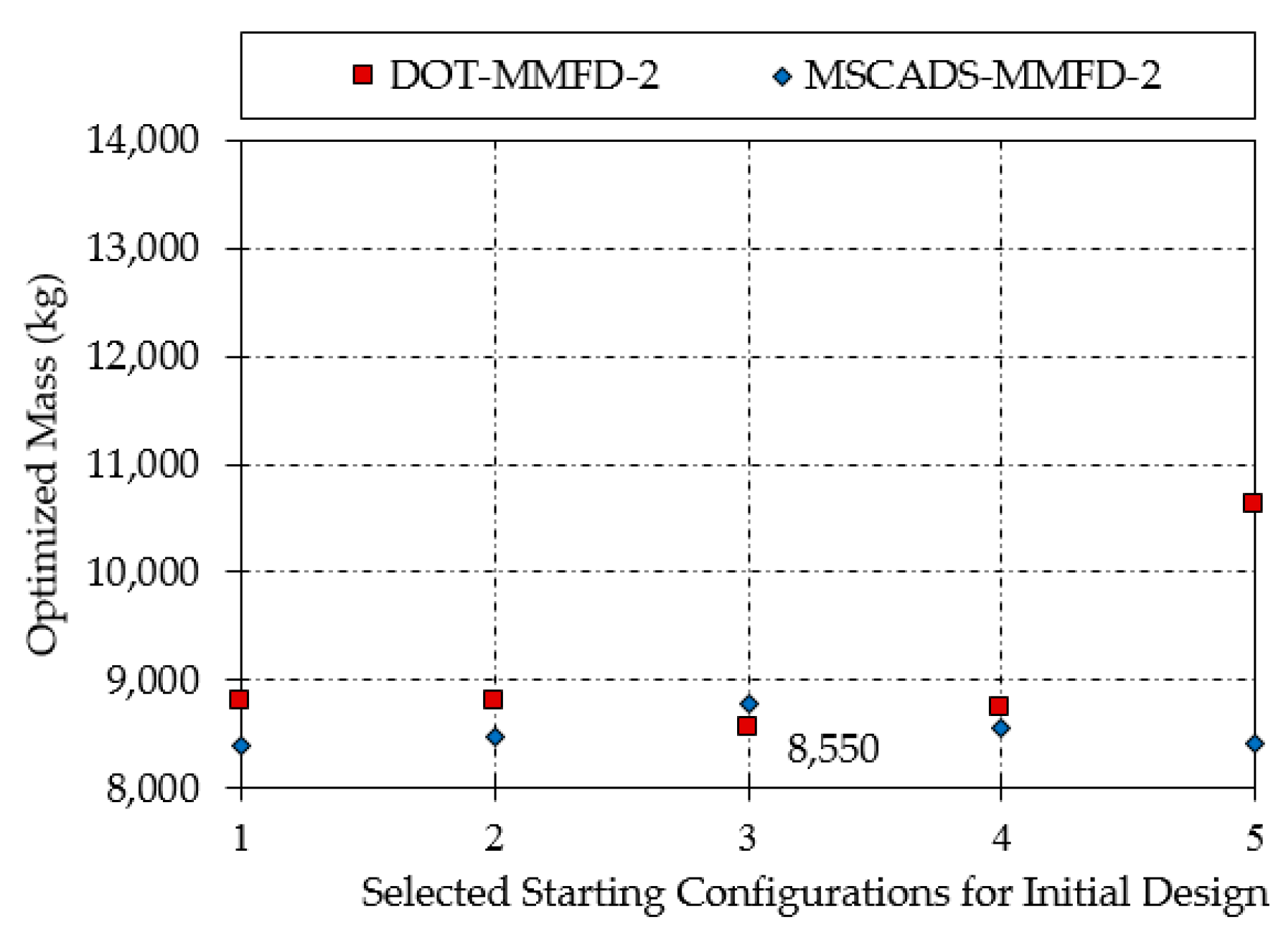
Figure 14 and Figure 15 illustrate the results of the first and second optimization iterations obtained using the DOT and MSCADS algorithms for the composite CRM wingbox model.
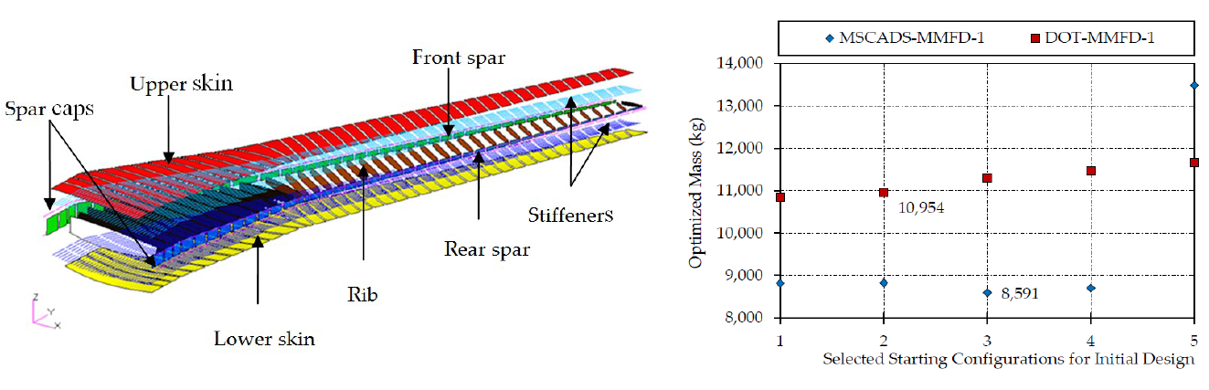
From the results presented in Table 5 and illustrated in Figure 14 and Figure 15, the same observations hold as we already mentioned in Table 3 and Figure 8 and Figure 9. However, the results in Table 5 show that the value of the objective function of the composite CRM wingbox is case-sensitive to both the choice of the optimization algorithm and the starting values for the design variables. For instance, using the MSCADS algorithm in the first run of the optimization obtained infeasible discrete solutions. On the other hand, by using the DOT algorithm in the first run, a feasible discrete design was obtained. Not only have the chances of finding feasible discrete solutions increased in the second run, but the value of the objective function against the initial optimized value has also improved. The minimum optimized mass of the composite CRM wingbox is obtained using the DOT-MMFD-2 iterative solution with a value of 8550 kg, compared to the initial optimized mass of 10,954 kg.
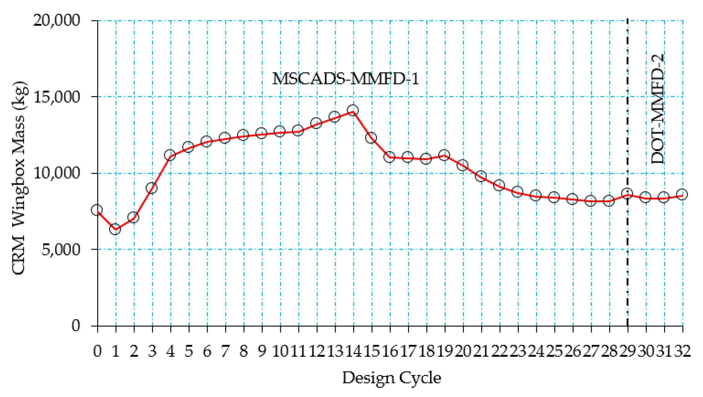
Figure 16 shows the history of the objective function as a function of the design cycles for the composite CRM wingbox model. As can be seen from Figure 16, while hard convergence to an optimum and feasible discrete solution is not achieved in 29 design cycles for the composite CRM wingbox using the MSCADS-MMFD-1 solution, a hard converged solution is founded using the DOT-MMFD-2 solution in three design cycles. The 0th design cycle corresponds to the initial mass of the wingbox model, which is based on the starting values of the design variables. Continuous optimization for the composite wingbox model is achieved in 28 design iterations using MSCADS-MMFD-1 and in two design iterations using the DOT-MMFD-2 solution. The 29th and 32nd design cycles, as shown in Figure 16, correspond to the rounded-up discrete solution.
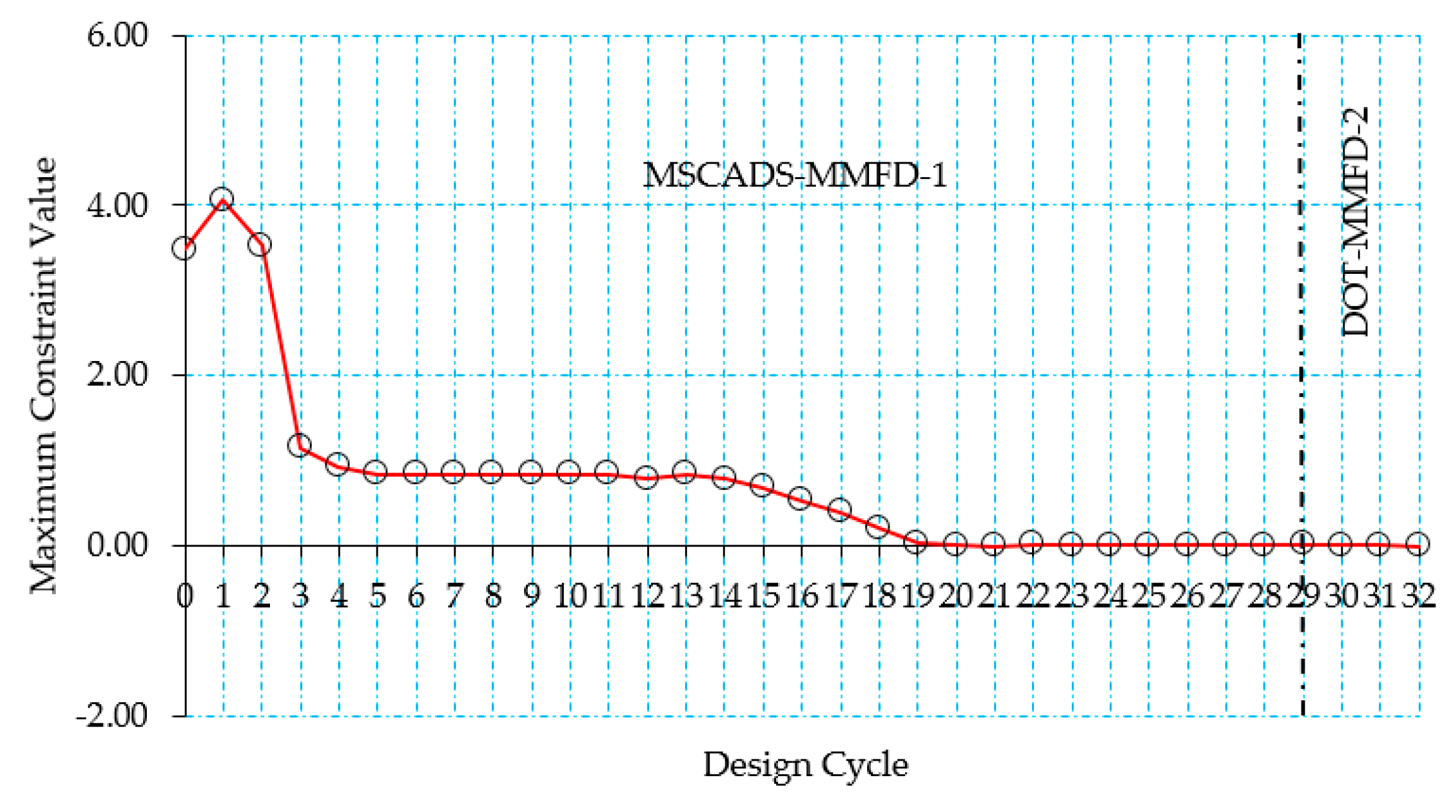
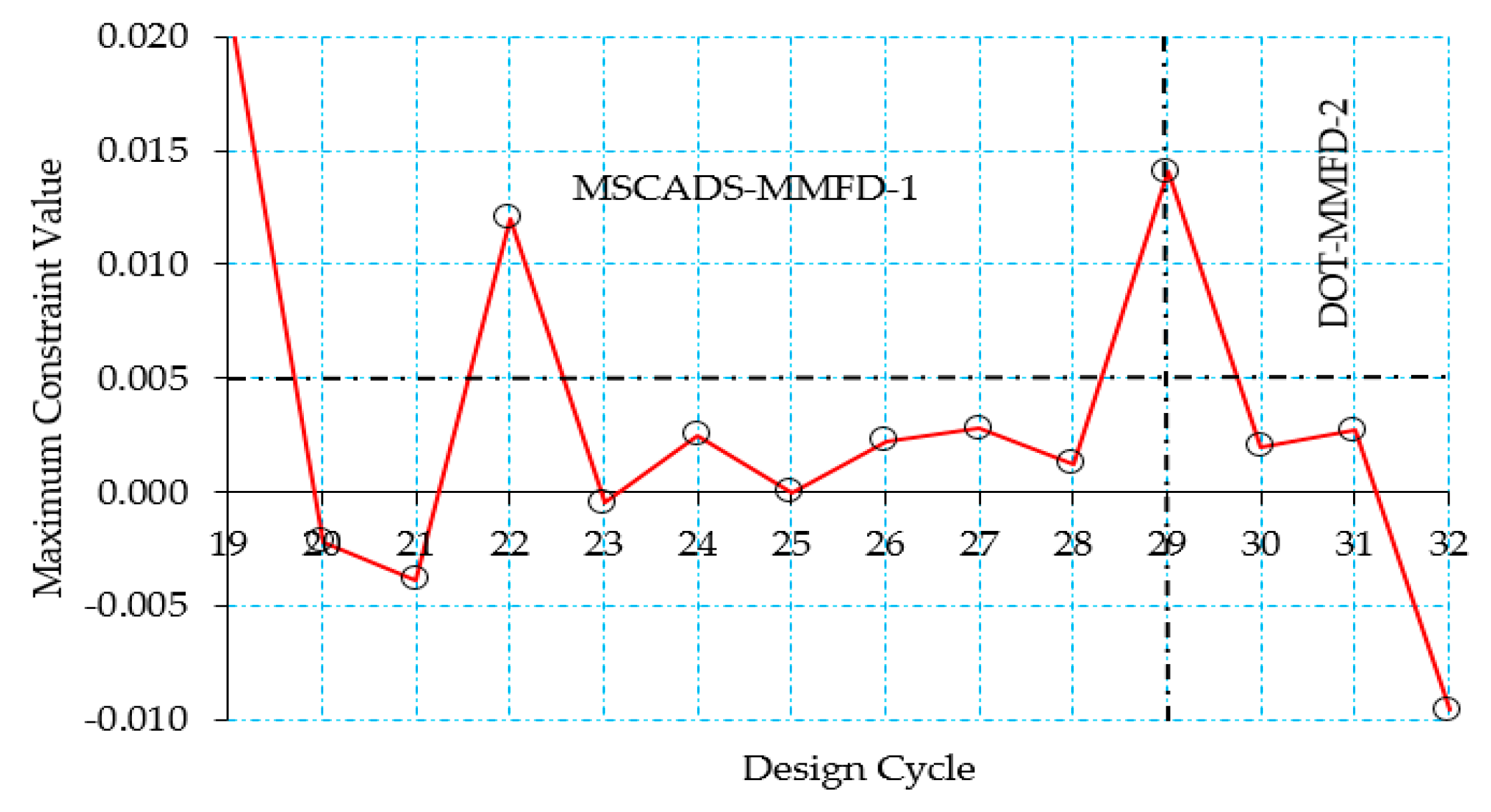
Figure 17 and Figure 18 (zoomed region) show the history of the maximum constraint value with respect to the design cycles for the composite CRM wingbox model. As can be seen from Figure 17, the initial constraints are violated because the maximum constraint value is greater than the allowable value of 0.005. The 0th design cycle corresponds to the initial mass of the wingbox, which is calculated using half of the upper bound value of the design variables. In this case, the search direction has been chosen to reduce the constraint violation. Thus, the objective function value will increase, since the first priority is to overcome the constraint violations. By using a number of fully stressed design cycles at the beginning of the optimization process, the large value of the maximum constraint violation is reduced to a smaller value during the 12th design cycle, as can be seen from Figure 17. After this happens, the value of the objective function starts to increase, allowing additional reduction in the maximum constraint violation value (see Figure 17 and Figure 18, design cycles 13 and 14) before it starts to decrease again allowing additional reduction in the wingbox optimized mass while trying to overcome the constraint violations in this direction.
6. Conclusions
A practical optimization procedure in an industrial context was developed as part of the sizing optimization process, with enhanced features in solving large-scale nonlinear structural optimization problems, incorporating an effective initial design variable value generation scheme based on the concept of the fully stressed design. The results of the foregoing case studies demonstrate that the application of the practical optimization procedure increased the efficacy of the local search algorithms of MSC Nastran Sol 200 in obtaining discrete, feasible, and optimal wingbox mass designs. Its performance is illustrated through the application of two case studies in which the metallic and composite wingbox models are optimized for a design of minimum mass. The results of the metallic CRM wing optimization study showed that the optimized masses obtained using MSCADS-MMFD-2 and DOT-MMFD-2 were very close to each other, with only slight favorable overall mass on behalf of the masses obtained using MSCADS-MMFD-2. On the other hand, the results of the composite CRM wing optimization study showed that when DOT-MMFD-1 is used, optimized wingbox configurations had significant mass penalties compared to the results obtained using MSCADS-MMFD-1. However, MSCADS-MMFD-1 solutions converged to infeasible discrete solutions. By using DOT-MMFD-2 and MSCADS-MMFD-2 iterative procedures, feasible discrete solutions were obtained and the mass penalties were decreased. Therefore, it can be revealed that the change in the optimized mass value—as a consequence of using different starting values for the design variables, as well as switching between different gradient-based algorithms in deriving the local optimum at each iteration step—is more appreciable in the case of the composite construct than in the case of the metallic construct. It is anticipated, therefore, that each optimization algorithm will have completely different search routes from the initial to final points, with the output as the solution. Moreover, using composite construction materials will dramatically alter the size of the design space, thereby increasing the number of solutions available to the designer, with the aim of improving the overall structural performance of the wing components.
Author Contributions
Odeh Dababneh performed all simulations and wrote the manuscript. Timoleon Kipouros and James F. Whidborne provided guidance and feedback on the results presented in the paper.
Conflicts of Interest
The authors declare no conflict of interest.
Appendix A.
This appendix presents an overview of the basic mathematical programming as applied to optimization tasks. In Appendix A.1 the numerical searching process for an optimum solution using function gradients is described. Appendix A.2 provides description of the concept of active and violated constraints.
Appendix A.1. Numerically Searching for an Optimum and Gradients Calculation
The optimization algorithms in MSC Nastran belong to a family of methods generally referred to as ‘gradient-based’, since they use function gradients in addition to function values in order to assist in the numerical search for an optimum. The numerical search process can be summarized as follows: for a given point in the design space, we determine the gradients of the objective function and its constraints, and use this information to determine a search direction. We then proceed in this direction as far as possible, after which we investigate to see if we are at an optimum point. If we are not, we repeat the process until we can make no further improvement in our objective without violating any of the constraints.
The first step in a numerical search procedure is determining the direction in which to search. The situation may be somewhat complicated if the current design is infeasible (with one or more violated constraints) or if one or more constraints are critical. For an infeasible design, we are outside of one of the fences, to use a hill analogy. In the case of a critical design, we are standing immediately adjacent to a fence. In general, we need to know at least the gradient of our objective function and perhaps some of the constraint functions as well. The process of taking small steps in each of the design variable directions (supposing we are not restricted by the fences for this step) corresponds exactly to the mathematical concept of a first-forward finite difference approximation of a derivative. For a single independent variable, the first-forward difference is given by
where the quantity represents the small step taken in the direction x. For the most practical design tasks, we are usually concerned with a vector of design variables. The resultant vector of partial derivatives, or gradient, of the function can be written as
where each partial derivative is a single component of the dimensional vector.
Physically, the gradient vector points uphill, or in the direction of increasing objective function. If we want to minimize the objective function, we will actually move in a direction opposite to that of the gradient. The steepest descent algorithm searches in the direction defined by the negative of the objective function gradient, or
Proceeding in this direction reduces the function value most rapidly. is referred to as the search vector.
MSC Nastran uses the steepest descent direction only when none of the constraints are critical or violated; even then, it is only used as the starting point for other, more efficient search algorithms. The difficulty in practice stems from the fact that, although the direction of steepest descent is usually an appropriate starting direction, subsequent search directions often fail to improve the objective function significantly. In MSC Nastran, more efficient methods, which can be generalized for the cases of active and/or violated constraints, are usually used.
Once a search direction has been determined, we proceeded ‘downhill’ until we collided with a fence, or until we reached the lowest point along our current path. It is important to note that this requires us to take a number of steps in this given direction, which is equivalent to a number of function evaluations in numerical optimization. For a search direction and a vector of design variables , the new design at the conclusion of our search in this direction can be written as
where is the initial vector of design variables, is the search vector, and is the value of the search parameter α that yields the optimal design in the direction defined by . Equation (A4), represents a one-dimensional search since the update on depends only on the single scalar parameter α. This relation allows us to update a potentially huge number of design variables by varying the single parameter α. When we can no longer proceed in this search direction, we have the value of α which represents the move required to reach the best design possible for this particular direction. This value is defined as . The new objective and constraints can now be expressed as
From this new point in the design space, we can again compute the gradients and establish another search direction based on this information. Again, we will proceed in this new direction until no further improvement can be made, repeating the process if necessary. At a certain point, we will not be able to establish a search direction that can yield an improved design. We may be at the bottom of the hill, or we may have proceeded as far as possible without crossing over a fence. In the numerical search algorithm, it is necessary to have some formal definition of an optimum. Any trial design can then be measured against this criterion to see if it is met, and if an optimum has been found. This required definition is provided by the Kuhn–Tucker conditions.
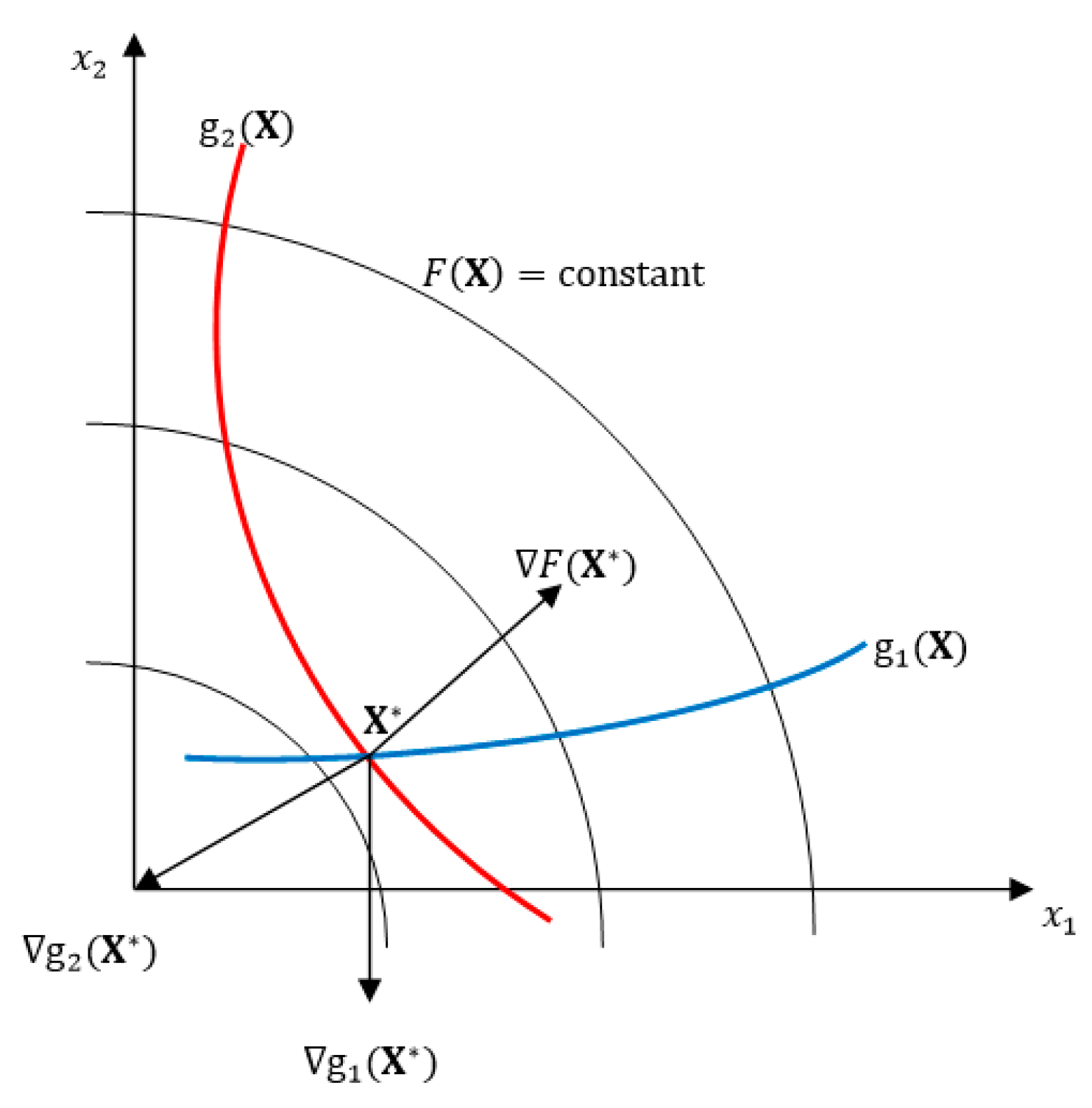
Figure A1 shows a two design variable space with constraints and and the objectives function . The constraint boundaries are those curves for which the constraint values are both zero. A few contours of constant objective are shown as well; these can be thought of as contour lines drawn along constant elevations of the hill. The optimum point in this example is the point which lies at the intersection of the two constraints. This location is shown as .
Figure A1.
Kuhn–Tucker condition at a constrained optimum.

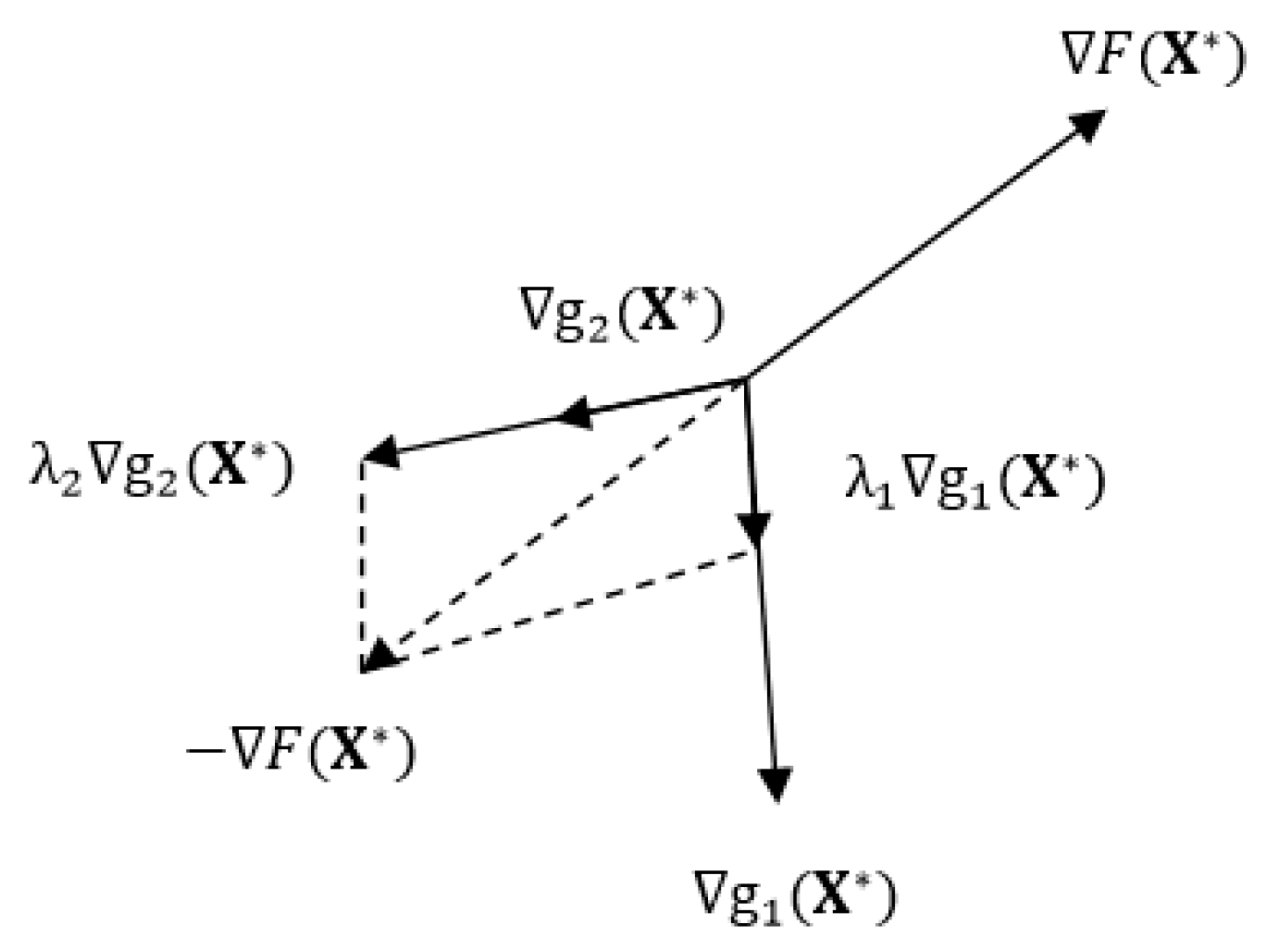
If we compute the gradients of the objective and the two active constraints at the optimum, we see that they all point off roughly in different directions (it should be remembered that function gradients point in the direction of increasing function values). For this situation—a constrained optimum—the Kuhn–Tucker conditions state that the vector sum of the objective and all active constraints must be equal to zero given an appropriate choice of multiplying factors. These factors are called the Lagrange multipliers. Constraints which are not active at the proposed optimum are not included in the vector summation.
Figure A2 shows this to be the case, where and are the values of the Lagrange multipliers that enable the zero vector sum condition to be met. It is likely that we could convince ourselves that this condition could not be met for any other point in the neighboring design space.
Figure A2.
Graphical interpretation of Kuhn–Tucker conditions.

The Kuhn–Tucker conditions are useful even if there are no active constraints at the optimum. In this case, only the objective function gradient is considered, and this is identically equal to zero; any finite move in any direction will not decrease the objective function. A zero objective function gradient indicates a stationary condition. Not only are the Kuhn–Tucker conditions useful in determining whether we have achieved an optimal design, but they are also physically intuitive. The optimizer tests the Kuhn–Tucker conditions in connection with the search direction determination algorithm.
Appendix A.2. Numerically Identifying the Active and Violated Constraints
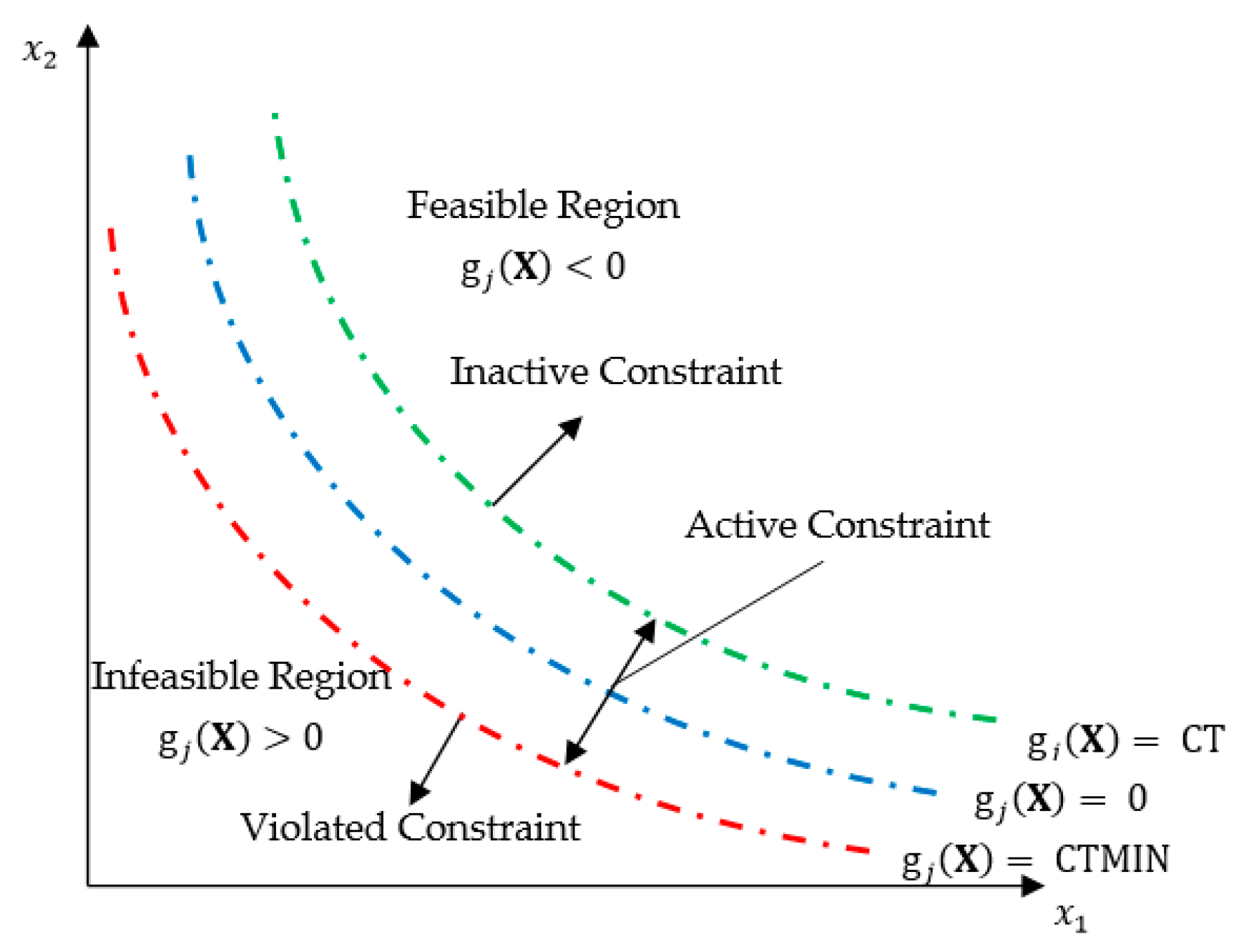
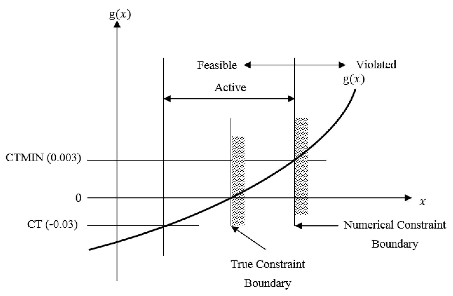
The optimization algorithm determines which of the retained constraints are violated and which are active. The constraints that are neither active nor violated can be ignored in the gradient evaluation. This reduces the amount of computations and computer memory required, as well as the size of the mathematical programming task. Figure A3 illustrates the concept of active and violated constraints for a single inequality constraint in a simple two-design variable space. Figure A4 presents the same information in a plot of a constraint value as a function of a single design variable or search direction. A constraint is considered active if its numerical value exceeds CT. The default value for CT is −0.03, but this can be changed by the user. Once a constraint is active, its gradient is included in the search direction computation. An active constraint may subsequently become inactive if its value falls below CT.
Figure A3.
Active and violated constraints.

Figure A4.
CT and CTMIN.

The optimizer designates a constraint as violated if its value is greater than CTMIN. The CTMIN default is 0.003, as seen in Figure A4. Thus, a small constraint violation (three-tenths of one percent, by default) is tolerated.
References
- Brennan, J. Integrating Optimization into the Design Process. In Proceedings of the Altair HyperWorks Technology Showcase, London, UK, 1999. [Google Scholar]
- Cervellera, P. Optimization Driven Design Process: Practical Experience on Structural Components. In Proceedings of the 14th Convegno Nazionae ADM, Bari, Italy, 31 August–2 September 2004. [Google Scholar]
- Gartmeier, O.; Dunne, W.L. Structural Optimization in Vehicle Design Development. In Proceedings of the MSC Worldwide Automotive Conference, Munich, Germany, 20–22 September 1999. [Google Scholar]
- Krog, L.; Tucker, A.; Rollema, G. Application of Topology, Sizing and Shape Optimization Methods to Optimal Design of Aircraft Components. In Proceedings of the 3rd Altair UK HyperWorks Users Conference, London, UK, 2002; Available online: http://www.soton.ac.uk/~jps7/Aircraft%20Design%20Resources/manufacturing/airbus%20wing%20rib%20design.pdf (accessed on 4 January 2018).
- Krog, L.; Tucker, A.; Kempt, M.; Boyd, R. Topology Optimization of Aircraft Wing Box Ribs, AIAA-2004-4481. In Proceedings of the 10th AIAA/ISSMO Symposium on Multidisciplinary Analysis and Optimization, Albany, NY, USA, 30 August–1 September 2004. [Google Scholar]
- Schumacher, G.; Stettner, M.; Zotemantel, R.; O’Leary, O.; Wagner, M. Optimization Assisted Structural Design of New Military Transport Aircraft, AIAA-2004-4641. In Proceedings of the 10th AIAA MAO Conference, Albany, NY, USA, 30 August–1 September 2004. [Google Scholar]
- Wasiutynski, Z.; Brandt, A. The Present State of Knowledge in the Field of Optimum Design of Structures. Appl. Mech. Rev. 1963, 16, 341–350. [Google Scholar]
- Schmit, L.A. Structural synthesis—Its genesis and development. AIAA J. 1981, 19, 1249–1263. [Google Scholar] [CrossRef]
- Vanderplaats, G.N. Structural Optimization-Past, Present, and Future. AIAA J. 1982, 20, 992–1000. [Google Scholar] [CrossRef]
- Maxwell, C. Scientific Papers. 1952, 2, 175–177. Available online: http://strangebeautiful.com/other-texts/maxwell-scientificpapers-vol-ii-dover.pdf (accessed on 21 April 2015).
- Michell, A.G. The limits of economy of material in frame-structures. Lond. Edinb. Dublin Philos. Mag. J. Sci. 1904, 8, 589–597. [Google Scholar] [CrossRef]
- Shanley, F. Weight-Strength Analysis of Aircraft Structures; Dover Publication Inc.: New York, NY, USA, 1950. [Google Scholar]
- Dantzig, G.B. Programming in Linear Structures; Comptroller, U.S.A.F: Washington, DC, USA, 1948. [Google Scholar]
- Heyman, J. Plastic Design of Beams and Frames for Minimum Material Consumption. Q. Appl. Math. 1956, 8, 373–381. [Google Scholar] [CrossRef]
- Schmit, L.A. Structural Design by Systematic Synthesis. In Proceedings of the 2nd Conference ASCE on Electronic Computation, Pittsburgh, PA, USA, 8–10 September 1960; American Society of Civil Engineers: Reston, VA, USA, 1960; pp. 105–122. [Google Scholar]
- Venkayya, V.B. Design of Optimum Structures. Comput. Struct. 1971, 1, 265–309. [Google Scholar] [CrossRef]
- Prager, W.; Taylor, J.E. Problems in Optimal Structural Design. J. Appl. Mech. 1968, 36, 102–106. [Google Scholar] [CrossRef]
- Schmit, L.A.; Farshi, B. Some Approximation Concepts for Structural Synthesis. AIAA J. 1974, 12, 692–699. [Google Scholar] [CrossRef]
- Starnes, J.R., Jr.; Haftka, R.T. Preliminary Design of Composite Wings for Buckling, Stress and Displacement Constraints. J. Aircr. 1979, 16, 564–570. [Google Scholar] [CrossRef]
- Gellatly, R.H.; Berke, L.; Gibson, W. The use of Optimality Criterion in Automated Structural Design. In Proceedings of the 3rd Air Force Conference on Matrix Methods in Structural Mechanics, Wright Patterson AFB, OH, USA, 19–21 October 1971. [Google Scholar]
- Brugh, R.L. NASA Structural Analysis System (NASTRAN); National Aeronautics and Space Administration (NASA): Washington, DC, USA, 1989.
- Haug, E.J.; Choi, K.K.; Komkov, V. Design Sensitivity Analysis of Structural Systems, 1st ed.; Academic Press: Cambridge, MA, USA, 1986; Volume 177. [Google Scholar]
- Haftka, R.T.; Adelman, H.M. Recent developments in structural sensitivity analysis. Struct. Optim. 1989, 1, 137–151. [Google Scholar] [CrossRef]
- Arora, J.S.; Huang, M.W.; Hsieh, C.C. Methods for optimization of nonlinear problems with discrete variables: A review. Struct. Optim. 1994, 8, 69–85. [Google Scholar] [CrossRef]
- Sandgren, E. Nonlinear integer and discrete programming for topological decision making in engineering design. J. Mech. Des. 1990, 112, 118–122. [Google Scholar] [CrossRef]
- Thanedar, P.B.; Vanderplaats, G.N. Survey of Discrete Variable Optimization for Structural Design. J. Struct. Eng. ASCE 1995, 121, 301–306. [Google Scholar] [CrossRef]
- Moore, G.J. MSC Nastran 2012 Design Sensitivity and Optimization User’s Guide; MSC Software Corporation: Santa Ana, CA, USA, 2012. [Google Scholar]
- Gill, P.; Murray, W.; Saunders, M. SNOPT: An SQP Algorithm for Large Scale Constrained Optimization. SIAM J. Optim. 2002, 12, 979–1006. [Google Scholar] [CrossRef]
- Dennis, J.E., Jr.; Schnabel, R.B. Numerical Methods for Unconstrained Optimization and Nonlinear Equations; Prentice Hall: Englewood Cliffs, NJ, USA, 1983. [Google Scholar]
- Kim, H.; Papila, M.; Mason, W.H.; Haftka, R.T.; Watson, L.T.; Grossman, B. Detection and Repair of Poorly Converged Optimization Runs. AIAA J. 2001, 39, 2242–2249. [Google Scholar] [CrossRef]
- Klimmek, T. Parametric Set-Up of a Structural Model for FERMAT Configuration for Aeroelastic and Loads Analysis. J. Aeroelast. Struct. Dyn. 2014, 3, 31–49. [Google Scholar]
- Jutte, C.V.; Stanford, B.K.; Wieseman, C.D. Internal Structural Design of the Common Research Model Wing Box for Aeroelastic Tailoring; Technical Report-TM-2015-218697; National Aeronautics and Space Administration (NASA): Hampton, VA, USA, 2015.
- Federal Aviation Administration (FAA). FAR 25, Airworthiness Standards: Transport Category Airplanes (Title 14 CFR Part 25). Available online: http://flightsimaviation.com/data/FARS/part_25.html (accessed on 15 January 2014).
- European Aviation Safety Agency (EASA). Certification Specifications and Acceptable Means of Compliance for Large Aeroplanes CS-25, Amendment 16. Available online: http://easa.europa.eu/system/files/dfu/CS-25 20Amdendment 16.pdf (accessed on 28 March 2015).
- ESDU. Computer Program for Estimation of Spanwise Loading of Wings with Camber and Twist in Subsonic Attached Flow. Lifting-Surface Theory. 1999. Available online: https://www.esdu.com/cgi-bin/ps.pl?sess=cranfield5_1160220142018cql&t=doc&p=esdu_95010c (accessed on 12 March 2014).
- Tomas, M. User’s Guide and Reference Manual for Tornado. 2000. Available online: http://www.tornado.redhammer.se/index.php/documentation/documents (accessed on 12 March 2014).
- Torenbeek, E. Development and Application of a Comprehensive Design Sensitive Weight Prediction Method for Wing Structures of Transport Category Aircraft; Delft University of Technology: Delft, The Netherlands, 1992. [Google Scholar]
- Jones, R.M. Mechanics of Composite Materials, 2nd ed.; Taylor & Francis: New York, NY, USA, 1999. [Google Scholar]
- Tsai, S.W.; Hahn, H.T. Introduction to Composite Materials; Technomic Publishing Co.: Lancaster, PA, USA, 1980. [Google Scholar]
- Kassapoglou, C. Review of Laminate Strength and Failure Criteria, in Design and Analysis of Composite Structures: with Applications to Aerospace Structures; John Wiley & Sons Ltd.: Oxford, UK, 2013. [Google Scholar]
- Niu, M.C. Composite Airframe Structures, 3rd ed.; Conmilit Press Ltd.: Hong Kong, China, 2010. [Google Scholar]
- Oliver, M.; climent, H.; Rosich, F. Non Linear Effects of Applied Loads and Large Deformations on Aircraft Normal Modes. In Proceedings of the RTO AVT Specialists’ Meeting on Structural Aspects of Flexible Aircraft Control, Ottawa, ON, Canada, 18–20 October 1999. [Google Scholar]
- Liu, Q.; Mulani, S.; Kapani, R.K. Global/Local Multidisciplinary Design Optimization of Subsonic Wing, AIAA 2014-0471. In Proceedings of the 10th AIAA Multidisciplinary Design Optimization Conference, National Harbor, MD, USA, 13–17 January 2014. [Google Scholar]
- Barker, D.K.; Johnson, J.C.; Johnson, E.H.; Layfield, D.P. Integration of External Design Criteria with MSC. Nastran Structural Analysis and Optimization. In Proceedings of the MSC Worldwide Aerospace Conference & Technology Showcase, Toulouse, France, 24–16 September 2001; MSC Software Corporation: Santa Ana, CA, USA, 2002. [Google Scholar]
- ASM Aerospace Specification Metals Inc. (ASM). ASM Aerospace Specification Metals, Aluminum 7050-T7451. 1978. Available online: http://asm.matweb.com/search/SpecificMaterial.asp?bassnum=MA7050T745 (accessed on 12 June 2014).
- ASM Aerospace Specification Metals Inc. (ASM). ASM Aerospace Specification Metals, Aluminum 2024-T3. 1978. Available online: http://asm.matweb.com/search/SpecificMaterial.asp?bassnum=%20MA2024T3 (accessed on 12 June 2014).
- Soni, S.R. Elastic Properties of T300/5208 Bidirectional Symmetric Laminates—Technical Report Afwal-Tr-80-4111; Materials Laboratory, Air Force Wright Aeronautical Laboratories, Air Force Systems Command: Dayton, OH, USA, 1980. [Google Scholar]
- MSC Patran Laminate Modeler User’s Guide; MSC Software Corporation: Santa Ana, CA, USA, 2008.
Figure 1.
Schematic diagram of the traditional approach to structural optimization.

Figure 2.
Schematic diagram of design modification process performed using approximate design model and finite element analysis.
Figure 2.
Schematic diagram of design modification process performed using approximate design model and finite element analysis.

Figure 3.
Schematic diagram of the structural optimization performed in MSC Nastran.

Figure 4.
Flowchart of the proposed practical optimization framework. FSD: Fully Stressed Design; DOT: Design Optimization Tool; MMFD: Modified Method of Feasible Directions.
Figure 4.
Flowchart of the proposed practical optimization framework. FSD: Fully Stressed Design; DOT: Design Optimization Tool; MMFD: Modified Method of Feasible Directions.

Figure 5.
Flowchart of the improved search for an optimum solution.

Figure 6.
Design optimization zones of the CRM wingbox.

Figure 7.
The CRM wingbox model used in the optimization study.

Figure 8.
Mass of the optimized metallic CRM wingbox using the first iterative procedure.

Figure 9.
Mass of the optimized metallic CRM wingbox using the second iterative procedure.

Figure 10.
Variation of the metallic CRM wingbox mass versus the design cycle—configuration #1.

Figure 11.
Maximum constraint value versus design cycle for the metallic CRM wingbox—configuration #1.
Figure 11.
Maximum constraint value versus design cycle for the metallic CRM wingbox—configuration #1.

Figure 12.
Zoomed region of the maximum constraint value for the metallic CRM wingbox—configuration #1.
Figure 12.
Zoomed region of the maximum constraint value for the metallic CRM wingbox—configuration #1.

Figure 13.
Schematic of the symmetric and balanced composite laminate.

Figure 14.
Mass of the optimized composite CRM wingbox using the first iterative procedure.

Figure 15.
Mass of the optimized composite CRM wingbox using the second iterative procedure.

Figure 16.
Variation of the composite CRM wingbox mass versus the design cycle—configuration #3.

Figure 17.
Maximum constraint value versus design cycle for the composite CRM wingbox—configuration #3.
Figure 17.
Maximum constraint value versus design cycle for the composite CRM wingbox—configuration #3.

Figure 18.
Zoomed region of maximum constraint value for the composite CRM wingbox—configuration #3.
Figure 18.
Zoomed region of maximum constraint value for the composite CRM wingbox—configuration #3.


Table 1.
Relevant data with respect to Common Research Model (CRM) aircraft.
| Description | Value |
|---|---|
| Maximum take-off mass | 260,000 kg |
| Maximum zero fuel mass | 19,500 kg |
| Main landing gear mass | 9620 kg |
| Engine mass (2×) | 15,312 kg |
| Maximum fuel mass | 131,456 kg |
| Wing gross area | 383.7 m2 |
| Wing span | 58.76 m |
| Aspect ratio | 9.0 |
| Root chord | 13.56 m |
| Tip chord | 2.73 m |
| Taper ratio | 0.275 |
| Leading edge sweep | 35.0° |
| Cruise speed | 193.0 m/s EAS |
| Dive speed | 221.7 m/s EAS |
| Cruise altitude | 10,668 m |
Table 2.
Material properties of aluminium alloys.
| Material Properties | 2024-T351 | 7050-T7451 |
|---|---|---|
| Modulus of elasticity | 73.1 GPa | 71.7 GPa |
| Shear modulus | 28 GPa | 26.9 GPa |
| Shear strength | 283 MPa | 303 MPa |
| Ultimate tensile strength | 469 MPa | 524 MPa |
| Yield tensile strength | 324 MPa | 469 MPa |
| Density | 2780 kg/m3 | 2830 kg/m3 |
| Poisson’s ratio | 0.33 | 0.33 |
Table 3.
Optimized masses of the metallic CRM wingbox with different optimization algorithms.
| Solution Type | Optimized Mass (kg) | ||||
|---|---|---|---|---|---|
| Min | 25% Max | 50% Max | 75% Max | Max | |
| MSCADS-MMFD-1 | 13,518 | 13,337 | 13,560 | 13,188 | 13,407 |
| DOT-MMFD-1 | 13,265 | 13,523 | 13,401 | 13,486 | 13,441 |
| MSCADS-MMFD-2 | 13,078 | 13,156 | 13,186 | 13,171 | 13,170 |
| DOT-MMFD-2 | 13,240 | 13,174 | 13,353 | 13,228 | 13,247 |
Table 4.
T300/N5208 composite material properties.
| Material Properties | T300/N5208 |
|---|---|
| Longitudinal modulus E11 | 181 GPa |
| Transverse modulus E22 | 10.3 GPa |
| In-plane shear modulus G12 | 7.17 GPa |
| Longitudinal tensile strength F1t | 1500 MPa |
| Longitudinal compressive strength F1c | 1500 MPa |
| Transverse tensile strength F2t | 40 MPa |
| Transverse compressive strength F2c | 246 MPa |
| In-plane shear strength F6 | 68 MPa |
| Density | 1600 kg/m3 |
| Major Poisson’s ratio ν12 | 0.28 |
Table 5.
Optimized masses of the composite CRM wingbox with different optimization algorithms.
| Solution Type | Optimized Mass (kg) | ||||
|---|---|---|---|---|---|
| Min | 25% Max | 50% Max | 75% Max | Max | |
| MSCADS-MMFD-1 | 8816 | 8824 | 8591 | 8704 | 13,486 |
| DOT-MMFD-1 | 10,837 | 10,954 | 11,289 | 11,465 | 11,665 |
| MSCADS-MMFD-2 | 8389 | 8480 | 8788 | 8564 | 8415 |
| DOT-MMFD-2 | 8798 | 8806 | 8550 | 8750 | 10,630 |
© 2018 by the authors. Licensee MDPI, Basel, Switzerland. This article is an open access article distributed under the terms and conditions of the Creative Commons Attribution (CC BY) license (http://creativecommons.org/licenses/by/4.0/).
Share and Cite
MDPI and ACS Style
Dababneh, O.; Kipouros, T.; Whidborne, J.F. Application of an Efficient Gradient-Based Optimization Strategy for Aircraft Wing Structures. Aerospace 2018, 5, 3. https://doi.org/10.3390/aerospace5010003
AMA Style
Dababneh O, Kipouros T, Whidborne JF. Application of an Efficient Gradient-Based Optimization Strategy for Aircraft Wing Structures. Aerospace. 2018; 5(1):3. https://doi.org/10.3390/aerospace5010003
Chicago/Turabian StyleDababneh, Odeh, Timoleon Kipouros, and James F. Whidborne. 2018. "Application of an Efficient Gradient-Based Optimization Strategy for Aircraft Wing Structures" Aerospace 5, no. 1: 3. https://doi.org/10.3390/aerospace5010003
Note that from the first issue of 2016, this journal uses article numbers instead of page numbers. See further details here.