The Efficiency of a Hybrid Flapping Wing Structure—A Theoretical Model Experimentally Verified

Abstract

To propel a lightweight structure, a hybrid wing structure was designed; the wing’s geometry resembled a rotor blade, and its flexibility resembled an insect’s flapping wing. The wing was designed to be flexible in twist and spanwise rigid, thus maintaining the aeroelastic advantages of a flexible wing. The use of a relatively “thick” airfoil enabled the achievement of higher strength to weight ratio by increasing the wing’s moment of inertia. The optimal design was based on a simplified quasi-steady inviscid mathematical model that approximately resembles the aerodynamic and inertial behavior of the flapping wing. A flapping mechanism that imitates the insects’ flapping pattern was designed and manufactured, and a set of experiments for various parameters was performed. The simplified analytical model was updated according to the tests results, compensating for the viscid increase of drag and decrease of lift, that were neglected in the simplified calculations. The propelling efficiency of the hovering wing at various design parameters was calculated using the updated model. It was further validated by testing a smaller wing flapping at a higher frequency. Good and consistent test results were obtained in line with the updated model, yielding a simple, yet accurate tool, for flapping wings design.

1. Introduction

For several decades, men have been designing and flying micro air vehicles (MAVs, vehicles with wing span less than 15 cm). Due to their small dimensions and low forward speed, the Reynolds numbers for MAVs are roughly between 5 × 10⁴ and 5 × 10⁵ [1]. Reynolds number is defined as the ratio between inertia forces and the viscous forces and therefore in the quoted range (5 × 10⁴ and 5 × 10⁵) the viscous force applied on the wing is more substantial than the inertial force, and the aerodynamic regime becomes unsteady. McMasters and Henderson [2] have shown a relevant alternation of the aerodynamics coefficients with both a decrease of lift, a decrease of lift-to-drag ratio and an increase of drag when the Reynolds number of the fixed wing is smaller than 10⁵. Therefore, a MAV design could not be inspired by full scale aircraft design methodology, and should be inspired by small flyers in nature—birds and insects.

A major progress has been made in understanding the aerodynamic of insects’ flight, due to new developments in high-speed videography, and computational modeling. It was discovered that most insects flap their wings back and forth to generate lift and thrust. The various flapping wing patterns have been investigated and illustrated in the literature [3,4,5]. To understand the motion of the wings, it is reiterated in the next lines.

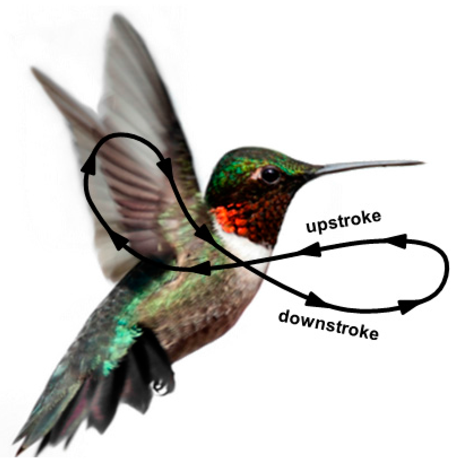
The forward motion of the wing, dorsal-to-ventral, is called the down stroke, and the backwards motion, ventral to dorsal, is called the upstroke. Towards the end of each stroke, the wing decelerates while increasing its angle of attack (AOA), until it reaches a complete stop at 90°, and accelerates back while decreasing its AOA. The flapping motion generates the figure eight (Figure 1), which is often approximated as a flapping plane. As insects fly forward, their flapping plane inclines forward [6].

Various unsteady lift mechanisms have been suggested [7,8,9,10,11,12,13] and have been validated in numerous experiments. In these experiments, a vast variety of wings, at different sizes and shapes, have been built to study the aerodynamics of flexible flapping wing at low Reynolds numbers. The instantaneous and mean lift and drag were measured as a function of various parameters such as wing’s structure, wing’s flexibility, wing’s aspect ratio, stroke amplitude and flapping frequency.

Most studies shared similar wing structure architecture—all were flat, built from a membrane stretched within a frame, inspired by the structure of insects’ wings. To obtain a high strength to weight ratio and a high Young’s modulus, the frame was often built from carbon or glass composite sheet [13,14,15], aluminum [16] or titanium alloy [17]. The membrane was manufactured from nylon [18], Mylar [18], paper [17], latex [13] or polyester [15].

The wing’s flexibility was discovered to play an important role in delaying stall and in generating a passive mechanism of adaptive washout. The flexibility is distinct in three categories: Spanwise, chordwise and twisting flexibility. Ifju et al. [13] investigated thirty different kinds of skeleton and membrane formation mounted on a MAV platform. The highest stall angles of attack, and thus the highest lift coefficients, were achieved by using the most chordwise flexible structures. Aono et al. [14] showed that wing flexibility could enhance the aerodynamic forces, using a combination of experimental and computational approaches. In particular, the elastic twisting of the wing was shown to produce substantially larger mean and instantaneous thrust due to shape deformation-induced changes at the effective AOA. Albeit, in the spanwise direction, a rigid leading edge was shown to produce larger lift coefficients compared to wings having flexible leading edges [17].

The wing’s aspect ratio was shown to have little effect on the aerodynamic performance of the air vehicle. Usherwood and Ellington [19] used five hawk moth wings, adjusted to aspect ratios ranging from 4.53 to 15.84, mounted on a motor, and measured “early” and “steady” horizontal and vertical forces on the rotor. They discovered that aspect ratio appears to have remarkably little effect on the force coefficients that can be achieved by revolving wings. However, it should be noted that in this study rotary wings were used instead of flapping wings. The use of rotary wings neglects the unsteady lift enhancement mechanisms, as well as inertial forces generated by the acceleration and deceleration of the wing. A study [20] conducted on various flyers ranging between 0.02 and 270 g body mass demonstrated that flyers with low aspect ratio wings generate a bit more lift per unit flight muscle mass. However, these results were not conclusive since different species were examined with different flap beat patterns.

The stroke amplitude of many insects in free-flight [21,22,23] ranges approximately from 90° to 180°. During flight, an insect can change the amplitude to control its aerodynamic force [24,25,26]. Sane and Dickinson [21] studied the effects of varying stroke amplitudes and other parameters using a dynamically scaled mechanical model of the fruit fly. Their results showed that the lift to drag ratio increases as the amplitude increases. Wu and Sun [27] validated their results by numerically solving the Navier–Stokes equations describing the unsteady aerodynamic forces of a model fruit fly wing. A similar conclusion can be derived by re-analyzing the data of Meng et al. [28], who calculated the aerodynamic forces generated by a corrugated flapping wing. In their study, the lift to drag ratio increases as the stroke amplitude increases, for all corrugated wing models.

Unlike the experimental tests presented in the literature on micro flapping wings (see typical examples in [29,30,31,32,33,34,35,36]), the present study aims at designing a macro flapping wing structure, in order to propel a light weight air vehicle, and to find the optimal parameters which will provide the best propelling efficiency in hovering. A hybrid wing structure was designed; the wing’s geometry resembled a rotor blade, and the wing’s flexibility resembled a flapping wing. The use of relative ”thick” airfoil made it possible to achieve higher strength to weight ratio by increasing the wing’s moment of inertia. In order to find the best design parameters, a simplified analytical model was developed to describe the propelling efficiency. This model was improved empirically based on the experimental data, and was validated on a second set of experiments based on a smaller wing flapping at a higher frequency, yielding good results.

2. Preliminary Considerations

2.1. Wing Load, Profile and Dimensions

A 1 kg payload was chosen, relatively heavy, in order to simplify the manufacturing and measuring of the wing, despite the low efficiency of flapping wings at these sizes. According to Alerstam et al. [37] the wing load of birds that weigh between 1 and 10 kg is between 60 and 90 N/m². Since the synthetic wing is stiffer than the birds’, a wing load of 90 N/m² was chosen. Assuming a typical structure’s weight to payload ratio of 1.8, a wing area of 0.2 m² was needed. The aspect ratio was set to be 6 for a slender wing with high efficiency. These figures yielded a wing span of 1.1 m and a chord length of 0.185 m.

As the desired characteristics for the wing’s airfoil were thinness, symmetry, and compatibility for low Reynolds numbers, in order to resemble insect’s wings, the chosen airfoil was S9033. This SELIG airfoil is designed especially for low Reynolds numbers [38]. According to wind tunnel test results conducted by Kruger et al. [39], this airfoil will stall at an AOA of 7° at Reynolds number of 36,000.

2.2. Flapping Frequency

A linearly twisted rotating wing was assumed in order to minimize the induced drag and to obtain a constant distributed load along the wing. Two parameters: Minimum drag (Figure 2) and an un-stalled wing (Figure 3) were the constraints for the flapping frequency, yielding a value of 3 Hz. The flapping frequency of 3 Hz produces an effective AOAs smaller than 7°.Furthermore, this frequency (3 Hz) is far from the region where the drag increases exponentially. One should note that unlike the aerodynamics of a stationary wing, the frequency of a flapping wing affects the effective AOA of the wing. The explicit formulation for the effective AOA is derived in Section 3. Furthermore, one of the main lifting mechanisms for insect aerodynamics is the leading edge vortex [10]. Although this mechanism is highly effective at low Reynolds numbers, at high Reynolds number a stalled wing will only decrease its efficiency. Therefore, in this study, only small AOA’s were tested, there were no flow detachments at the leading edge, and the lift vortex was shed from the tip of the wing (as for the blade of a helicopter) and not from the leading edge (as for the wings of insects).

3. Wing Model

3.1. The Rotating Wing Model

The following equations are based on helicopters aerodynamics [40].

The distribution of the lift along the wing span is given by:

$$\frac{\partial L}{\partial r}=\frac{1}{2}\rho \cdot a\cdot c\left(r\right)\cdot U_T{\left(r\right)}^2\cdot {\alpha }_{eff}\left(r\right)$$

(1)

where $\rho$ is the density of the fluid, $a$ is the slope of the lift line, $c$ is the chord length, $U_T=\Omega \cdot r$ is the tangent velocity, $\Omega$ is the rotational velocity and ${\alpha }_{eff}$, the effective AOA, being composed of three components: The collective AOA (a constant AOA along the wing span), ${\alpha }_0$, the geometrical twist of the wing, ${\alpha }_{tw}$, and the angle of the induced velocity, $\phi$, can be written as:

$${\alpha }_{eff}={\alpha }_0+{\alpha }_{tw}-\phi$$

(2)

where the collective AOA, ${\alpha }_0$ is defined as:

$${\alpha }_0=3\cdot \left(\frac{2C_T}{\sigma \cdot a}+\frac{\lambda }{2}\right)$$

(3)

with C_T, the trust coefficient given by:

$$C_T=\frac{mg}{\rho \cdot \pi \cdot {\Omega }^2\cdot {r_2}^4}$$

(4)

while $r_2$ being the radius at the free tip of the rotating wing and $\lambda$, the inflow at hovering, being derived from the momentum equation, is written as:

$$\lambda =\sqrt{\frac{C_T}{2}}$$

(5)

The solidity, σ, is defined as:

$$\sigma =\frac{N_b\cdot c}{\pi \cdot r_2}$$

(6)

where $N_b$ is the number of blades.

The geometrical twist along the wing span is given by:

$${\alpha }_{tw}=\left({\alpha }_{tip}-{\alpha }_{root}\right)\frac{r-r_1}{r_2-r_1}$$

(7)

where $r_1$ is the radius at the hub. The angle of induced velocity is written as:

$$\phi =\frac{U_N}{U_T}$$

(8)

where $U_N=\lambda \cdot \Omega \cdot r_2$ is the normal velocity, assuming the wing has no vertical velocity, besides the inflow. The distribution of the drag along the wing is given by the following equation:

$$\frac{\partial D}{\partial r}=\frac{1}{2}\rho \cdot C\left(r\right)\cdot U_T{\left(r\right)}^2\cdot C_D+\frac{\partial L}{\partial r}\cdot \phi$$

(9)

The parasite drag, $D_p=0.5\cdot \rho \cdot C\cdot {U_T}^2\cdot C_D$, is caused by friction. The tangent velocity of the fluid, right next to the wing equals to the wing’s velocity, and decreases gradually towards the standing fluid far from the wing. Due to fluid’s viscosity, there are inter layer shear forces, which transfer the momentum from one layer of fluid to the next, and thus creating a parasite drag force on the wing.

The induced drag, $D_i=\left(\partial L/\partial r\right)\cdot \phi$, is caused by the diversion of the lift vector backwards by the induced velocity. In order to generate lift, the flow must be provided with a downward momentum. This downward velocity decreases the effective AOA and creates a lift component in the opposite direction of wing’s velocity, i.e., in the drag direction. Therefore, lift generation will always produce induced drag, even in an ideal frictionless world.

The total drag can be calculated by summing the drag along the wing span and along the sweep angle ($\theta$), to yield:

$$D=\frac{N_b}{\pi }\cdot {\displaystyle \underset{0}{\overset{\pi }{\int }}d\theta }{\displaystyle \underset{r_1}{\overset{r_2}{\int }}\frac{\partial D}{\partial r}dr}$$

(10)

3.2. The Flapping Wing Model

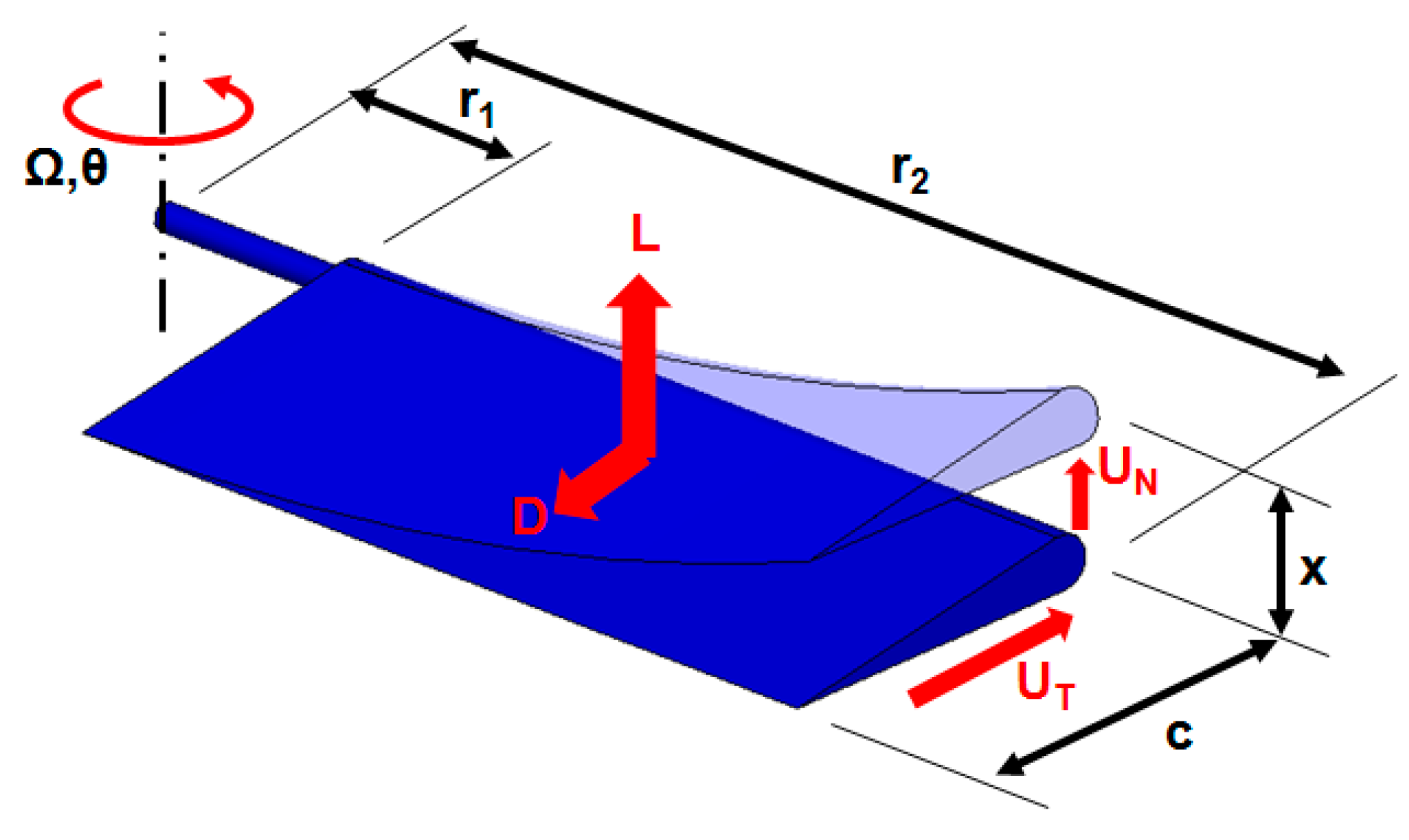
A simplified mathematical model (Figure 4) of the flapping motion aimed at capturing only the gross phenomena is next derived and presented. This model is inviscid, quasi-steady and does not take into consideration the complex lift mechanisms mentioned in the introduction. The choice to describe the aerodynamic behavior of the wing through moments was made to yield a direct relationship between the measured and the calculated parameters.

The wing is rotating around a vertical axis similar to a helicopter blade. At the end of the stroke the wing reverses its angle of attack, and rotates backwards. For insects, this back-and-forth movement generates the figure eight (Figure 1), which is often approximated as a flapping plane. The intuitive vertical movement, the up-and-down flap, is created passively due to the aerodynamic forces.

Based on Figure 4, where the x coordinate is parallel to the hub axis, one can write the various force components in x direction (out-of-plane) as:

$${\displaystyle \sum F_x=F_{aerodynamic}+}{F}_{structural}+F_{centripetal}+F_{inertial}=0$$

(11)

where the four force components are given by:

$$\begin{array}{ll}{F}_{aerodynamic}\equiv & L=\frac{N_b}{\pi }\cdot {\displaystyle \underset{0}{\overset{\pi }{\int }}d\theta }{\displaystyle \underset{r_1}{\overset{r_2}{\int }}\frac{\partial L}{\partial r}dr}=\frac{N_b}{\pi }\cdot {\displaystyle \underset{0}{\overset{\pi }{\int }}d\theta }{\displaystyle \underset{r_1}{\overset{r_2}{\int }}\frac{1}{2}\rho \cdot a\cdot C\cdot {U_T}^2\cdot {\alpha }_{eff}\cdot dr}\\ & =\frac{N_b}{\pi }\cdot {\displaystyle \underset{0}{\overset{\pi }{\int }}d\theta }{\displaystyle \underset{r_1}{\overset{r_2}{\int }}\frac{1}{2}\rho \cdot a\cdot C\cdot {U_T}^2\cdot \left({\alpha }_{tw}-\phi \right)\cdot dr}\end{array}$$

(12)

with:

$${\alpha }_{tw}=\left({\alpha }_{tip}-{\alpha }_{root}\right)\frac{r-r_1}{r_2-r_1}$$

(13)

$$\phi =\frac{U_N}{U_T}$$

(14)

$$U_T=\Omega \cdot r$$

(15)

$$F_{structural}=K_{s}X+K_{sd}\dot{X}$$

(16)

while the stiffness $K_s$ (static case) and $K_{sd}$ (dynamic case) are derived from the finite element analysis, by solving the case of a wing subjected to a concentrated load at its tip.

One should note that $F_{centripetal}$ is proportional to $\sin \left(x/r_2\right)$. Since $x<<r_2$, the centripetal force can be neglected.

$$F_{inertial}=M_i\ddot{X}$$

(17)

To calculate the mass $M_i$ we used the expression for the natural frequency of a cantilever beam [41], expressed as:

$${\omega }_{1,cantilever\_beam}=3.526\sqrt{\frac{E\cdot I}{m_{beam}\cdot L^3}}$$

(18)

and the expression for the natural frequency of a spring-suspended weight:

$${\omega }_{1,weight\_on\_spring}=\sqrt{\frac{K}{M_i}}$$

(19)

where the stiffness K is taken from the equation of the tip displacement of a cantilever beam subjected to a tip force, namely:

$$K=\frac{3EI}{L^3}$$

(20)

Equating between the natural frequency of the beam and the natural frequency of the weight (Equations (18) and (19)), yields:

$$M_i=\frac{3}{{\left(3.526\right)}^2}{m}_{beam}$$

(21)

Equation (12) can be simplified by assuming that the vertical flap movement is more substantial then the inflow (valid for relatively heavy wings at relatively low flapping frequency), namely the normal velocity, can be written as:

$$U_N=\lambda \cdot \Omega \cdot r_2+\dot{X}\cdot {\left(\frac{r}{r_2}\right)}^2\approx \dot{X}\cdot {\left(\frac{r}{r_2}\right)}^2$$

(22)

Substituting Equation (16), together with Equations (13)–(15) into Equation (12) yields:

$$F_{aerodynamic}=K_a{\Omega }^2+K_{ad}\Omega \dot{X}$$

(23)

where:

$$\begin{array}{l}{K}_a=\frac{1}{2}\rho aC{\displaystyle \underset{r_1}{\overset{r_2}{\int }}{r}^2\left[{\alpha }_{root}+\left({\alpha }_{tip}-{\alpha }_{root}\right)\frac{r-r_1}{r_2-r_1}\right]}dr\\ =\frac{1}{2}\rho \frac{\partial C_L}{\partial \alpha }C\left[\left({\alpha }_{root}+\left({\alpha }_{tip}-{\alpha }_{root}\right)\frac{r_1}{r_2-r_1}\right)\frac{\left({r_2}^3-{r_1}^3\right)}{3}+\left({\alpha }_{tip}-{\alpha }_{root}\right)\frac{\left({r_2}^4-{r_1}^4\right)}{4\left(r_2-r_1\right)}\right]\end{array}$$

(24)

and

$$K_{ad}=-\frac{1}{2}\rho \frac{\partial C_L}{\partial \alpha }C{\displaystyle \underset{r_1}{\overset{r_2}{\int }}r\cdot {\left(\frac{r}{r_2}\right)}^2}dr=-\frac{1}{8}\rho \frac{\partial C_L}{\partial \alpha }C\frac{\left({r_2}^4-{r_1}^4\right)}{r_2}$$

(25)

One should note that the above expressions could be obtained only under the following assumptions:

• There are no interactions between the wing and its wake, shed from the previous stroke.
• ${\alpha }_{root}$ and ${\alpha }_{tip}$ are constant and do not depend on the angular velocity $\Omega$.
• There is no chordwise deformation of the airfoil.

Substituting the various force components (Equations (16), (17) and (23)) into Equation (11), yields a second order differential equation:

$$\begin{array}{c}{K}_a{\Omega }^2+K_{ad}\Omega \dot{X}+K_{s}X+K_{sd}\dot{X}+M_i\ddot{X}=0\\ or\\ \begin{array}{c}\ddot{X}+\frac{K_{ad}\Omega +K_{sd}}{M_i}\dot{X}+\frac{K_s}{M_i}X=-\frac{K_a}{M_i}{\Omega }^2\end{array}\end{array}$$

(26)

By neglecting the damping effect in Equation (26) (the coefficient multiplying the velocity $\dot{X}$), an analytical solution for the vertical movement at the wing tip could be derived for a sinusoidal type angular velocity, $\Omega =A\cdot \sin \omega t$, having the following form:

$$X={\overline{C}}_1\sin {\omega }_{n}t+{\overline{C}}_2\cos {\omega }_{n}t-\frac{1}{2}K{A}^2\left(\frac{1}{{{\omega }_n}^2}-\frac{1}{{{\omega }_n}^2-4{\omega }^2}\cos 2\omega t\right)$$

(27)

where:

$${\omega }_n=\sqrt{\frac{K_s}{M_i}};\begin{array}{c}K=\frac{K_a}{M_i}.\end{array}$$

(28)

One should note that such a neglection is expected to cause a larger vertical movement, which will then be readjusted and corrected by the experimental results.

Each force is divided differently along the wing span, and a calculation of the moment should be the integral of the force along the span. In order to facilitate the calculation each force was replaced with a concentrated force at the tip of the wing, and thus simplifying the moment calculations.

The bending moment at the root of the wing (the out-of-plane bending moment) is calculated from the vertical displacement, namely:

$$\begin{array}{l}{M}_{vertical\_root}=-K_s\cdot X\cdot r_2\\ =-K_s{r}_2\left(C_1\sin {\omega }_{n}t+C_2\cos {\omega }_{n}t\right)+\frac{1}{2}\frac{K_a}{K_s}{A}^2\left(1-\frac{1}{1-4{\left(\frac{\omega }{{\omega }_n}\right)}^2}\cos 2\omega t\right)\cdot r_2\end{array}$$

(29)

3.3. The In-Plane Bending Moment

The sum of the in-plane bending moments around the root, with reference to the z axis can be written as:

$${\displaystyle \sum M_z=M_{aerodynamic}+}{M}_{motor}+M_{inertial}=0$$

(30)

where the aerodynamic moment can be written as:

$$M_{aerodynamic}=M_{aerodynamic\_parasite}+M_{aerodynamic\_induced}$$

(31)

with:

$$M_{aerodynamic\_parasite}=-{\displaystyle \underset{r_1}{\overset{r_2}{\int }}\frac{\partial D^{\prime }}{\partial r}}\cdot rdr=-\frac{1}{2}\rho c{\left(A\sin \omega t\right)}^2{\displaystyle \underset{r_1}{\overset{r_2}{\int }}{C}_D\cdot }{r}^{3}dr$$

(32)

and

$$\begin{array}{l}{M}_{aerodynamic\_induced}=-{\displaystyle \underset{r_1}{\overset{r_2}{\int }}\frac{\partial L}{\partial r}}\cdot \phi \cdot rdr=-{\displaystyle \underset{r_1}{\overset{r_2}{\int }}\frac{\partial L}{\partial r}}\cdot \left(\lambda +\frac{\dot{X}}{\Omega r}\frac{r^2}{{r_2}^2}\right)\cdot rdr\\ =-{\displaystyle \underset{r_1}{\overset{r_2}{\int }}\frac{\partial L}{\partial r}}\cdot \left(\sqrt{\frac{1}{2\rho \pi {\Omega }^2{r_2}^3}\frac{\partial L}{\partial r}}+\frac{\dot{X}}{\Omega r}\frac{r^2}{{r_2}^2}\right)\cdot rdr\\ =-{\displaystyle \underset{r_1}{\overset{r_2}{\int }}\left[{\left(\frac{\partial L}{\partial r}\right)}^{\frac{3}{2}}\sqrt{\frac{1}{2\rho \pi {\Omega }^2{r_2}^3}}+\frac{\partial L}{\partial r}\cdot \frac{\dot{X}}{\Omega r}\frac{r^2}{{r_2}^2}\right]}\cdot rdr\end{array}$$

(33)

$$\frac{\partial L}{\partial r}=\frac{1}{2}\rho c{\left(\Omega r\right)}^2\frac{\partial C_L}{\partial \alpha }\left[{\alpha }_{root}+\left({\alpha }_{tip}-{\alpha }_{root}\right)\frac{r-r_1}{r_2-r_1}+\frac{\dot{X}}{\Omega r}\frac{r^2}{{r_2}^2}\right]$$

(34)

The inertial moment can be written as:

$$M_{inertial}=-I\dot{\Omega }$$

(35)

while:

$$I=m{\displaystyle \underset{r_1}{\overset{r_2}{\int }}{r}^2}dr=\frac{1}{3}m\left({r_2}^3-{r_1}^3\right);\begin{array}{c}\dot{\Omega }=A\omega \cos \omega t.\end{array}$$

(36)

The in-plane bending moment at the root, can now be written as:

$$\begin{array}{l}{M}_{horizontal\_root}\equiv M_{motor}\\ =-M_{aerodynamic\_parasite}-M_{aerodynamic\_induced}-M_{inertial}\end{array}$$

(37)

To obtain non-dimensional moments, a division by $\left(0.5\cdot \rho c^2{{\Omega }_{\max }}^2{r_2}^3\right)$ is performed for all the moments involved.

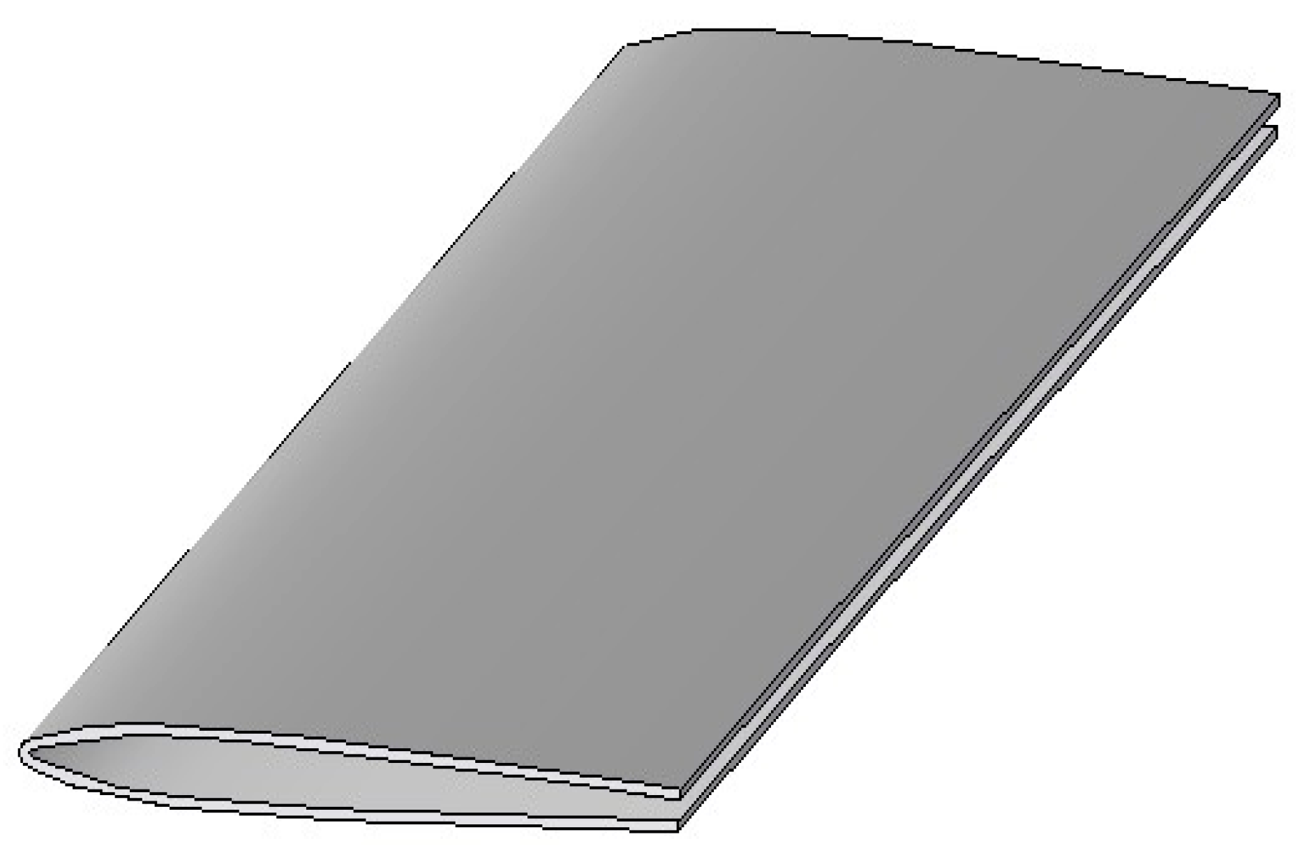
3.4. The Experimental Wing Model

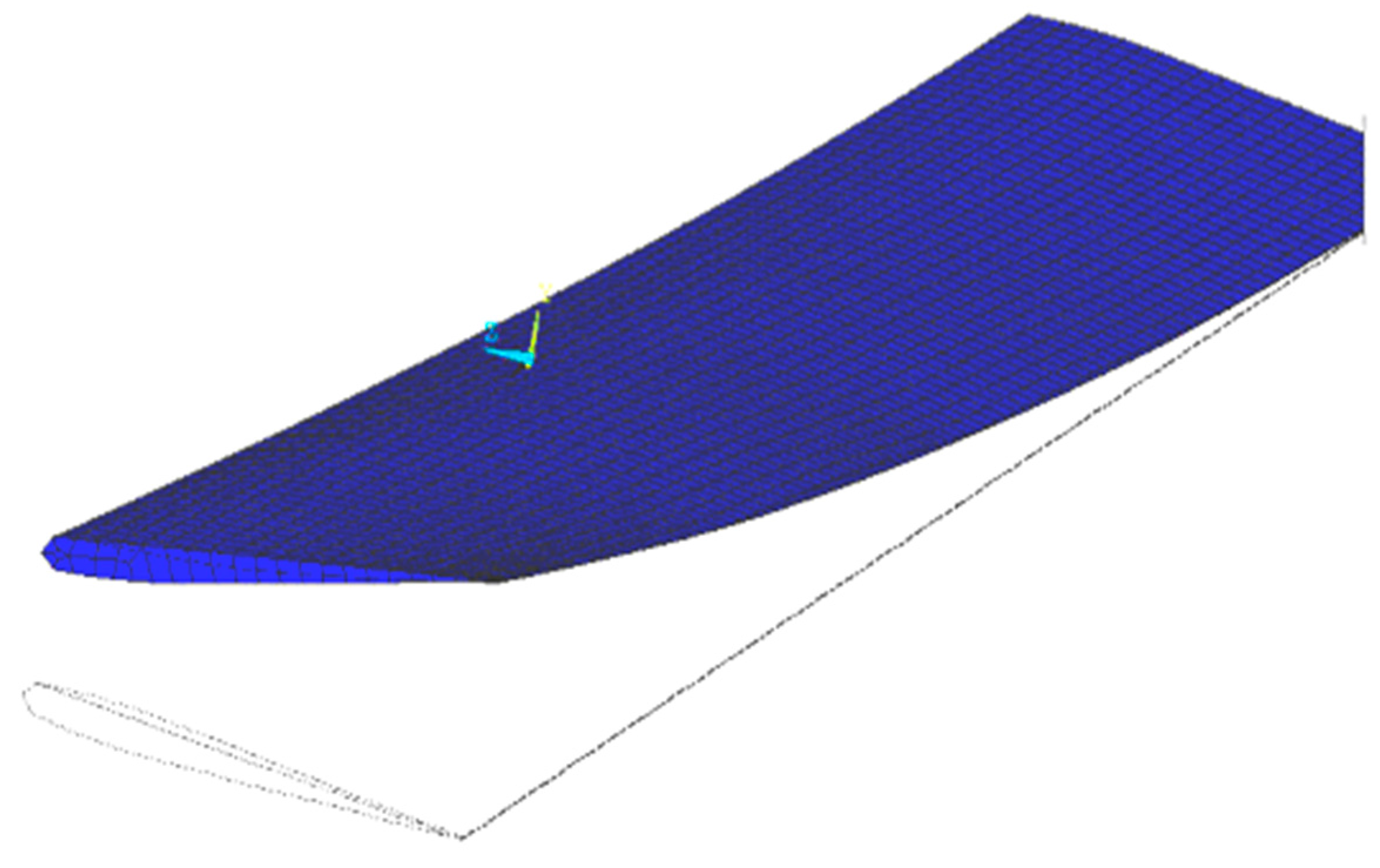
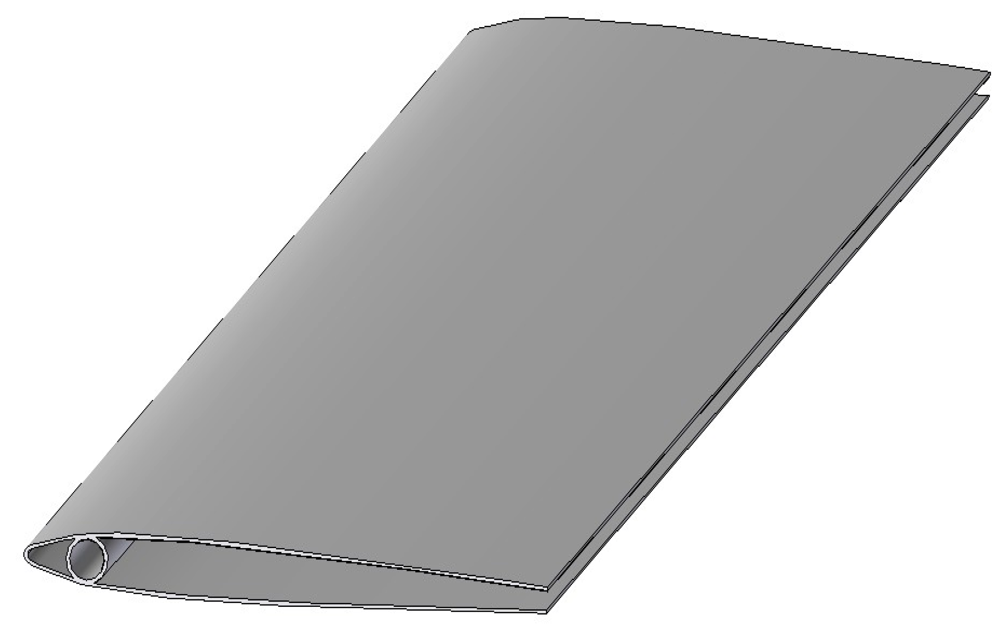
The first step was to obtain the twist along the wing (${\alpha }_{tw}$), as was a priory assumed by applying the aerodynamic loads calculated according to Equation (1) on the quarter of the wing’s chord (Figure 5). To get a wing stiff in bending while flexible in twisting, the wing was designed from a single fiberglass laminate, opened at its trailing edge (Figure 6). One should note that a similar structure was designed by Delaurier [42] to propel an ornithopter.

Using the ANSYS Finite Element Code [43] with designated laminated shell elements, the laminate composition of the wing was determined to be comprised from four layers (45°, −45°)_sym each at a thickness of 0.15 mm (Figure 7), yielding a total skin thickness of 0.6 mm. The parameters of each lamina were inserted into the element properties, according to the properties of the Young’s modulus in the fiber direction (E_x), the Young’s modulus perpendicular to the fiber (E_y) and the shear modulus of the laminate (G_xy). All parameters were validated by a calibration experiment (presented in Subsection 4.1).

To generate an axis of rotation for the wing, a 20 cm long fiberglass tube was glued inside the wing, close to its leading edge (Figure 8).

3.5. The Experimental Flapping Mechanism

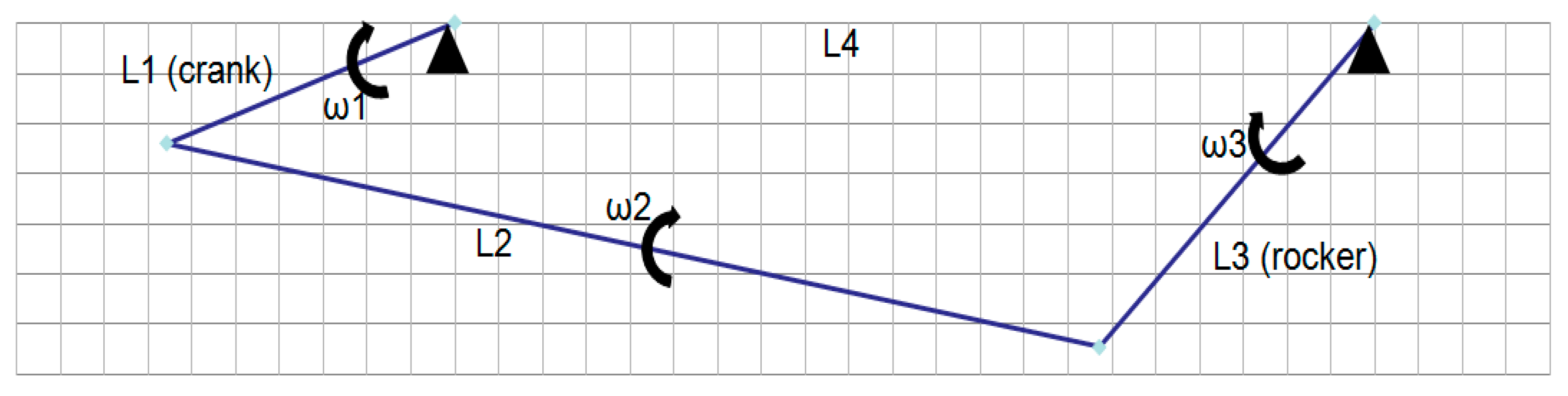
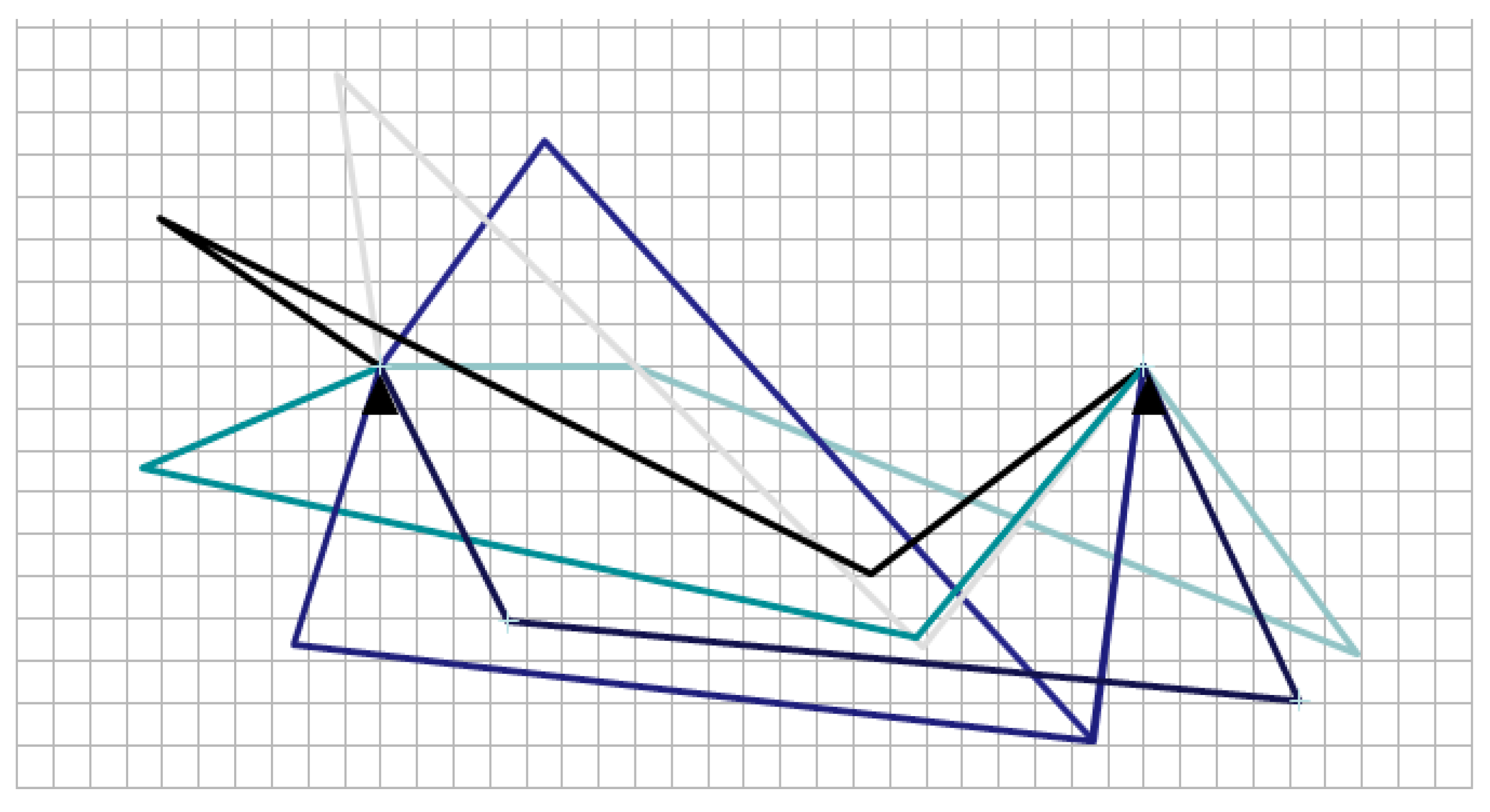
The flapping mechanism was a crank-rocker four-bar linkage (Figure 9). The crank was driven by an electric motor, at a constant angular velocity ${\omega }_1$. The wing was connected to the rocker, and flapped back and forth at an angular velocity ${\omega }_3$ (Figure 10). The length of the bars was set to produce flap amplitude of 90° (Figure 11).

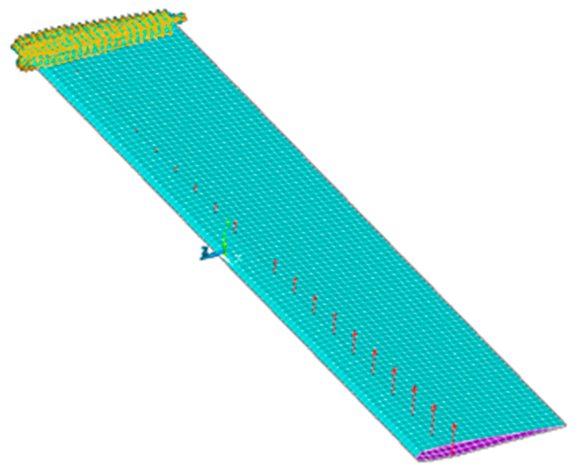
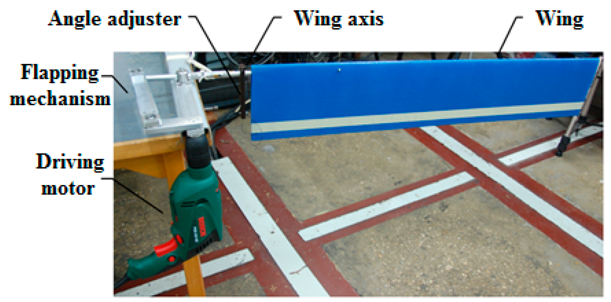
3.6. Test Set-Up

The test setup consisted of the following main parts (Figure 12): Wing, wing axis, angle adjuster, flapping mechanism and driving motor.

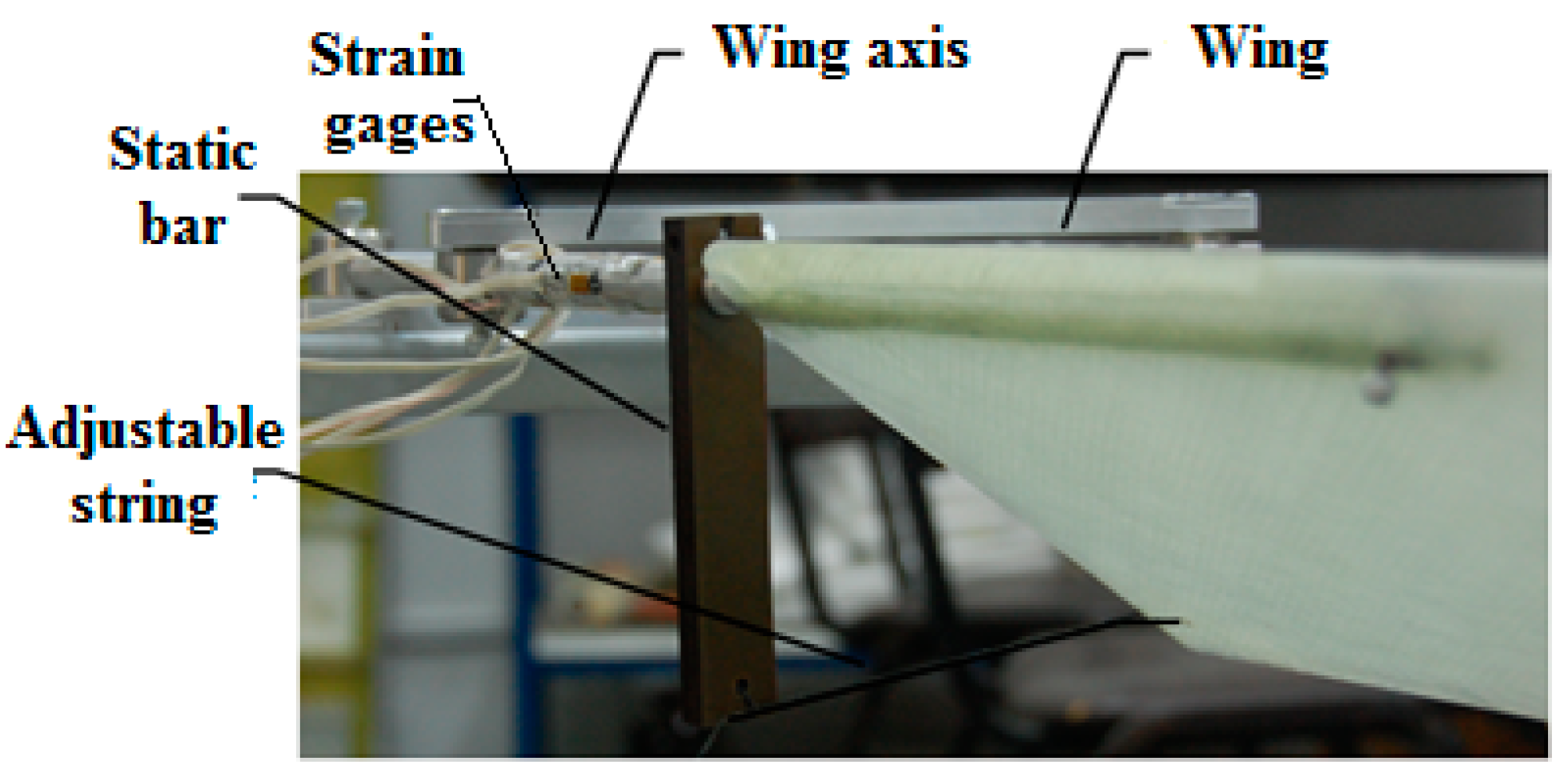
The flapping mechanism was attached to a test table. The driving motor (700W Bosch drill) was connected to the drive shaft of the flapping mechanism. The angle adjuster’s bar was tightened vertically to the wing axis. The wing axis was inserted into the wing, and a string was tied between the wing’s trailing edge and the angle adjuster’s bar (Figure 12), thus defining the minimum AOA at the root of the wing. Two pairs of strain gages were bonded on the wing axis (at 90° between the two pairs) (Figure 13), enabling the readings of in-plane and out-of-plane bending moments. A linear variable differential transformer (LVDT) was used to measure the sweep angle of the wing, throughout its movement. The time derivative of the sweep angle yielded the angular velocity of the wing. The vertical displacement of the wing was measured using a laser rangefinder placed statically above the wing tip, while the angle of attack at the wing tip was defined by measuring the upper wing camber with the same laser rangefinder.

4. Results

4.1. Structural Analysis

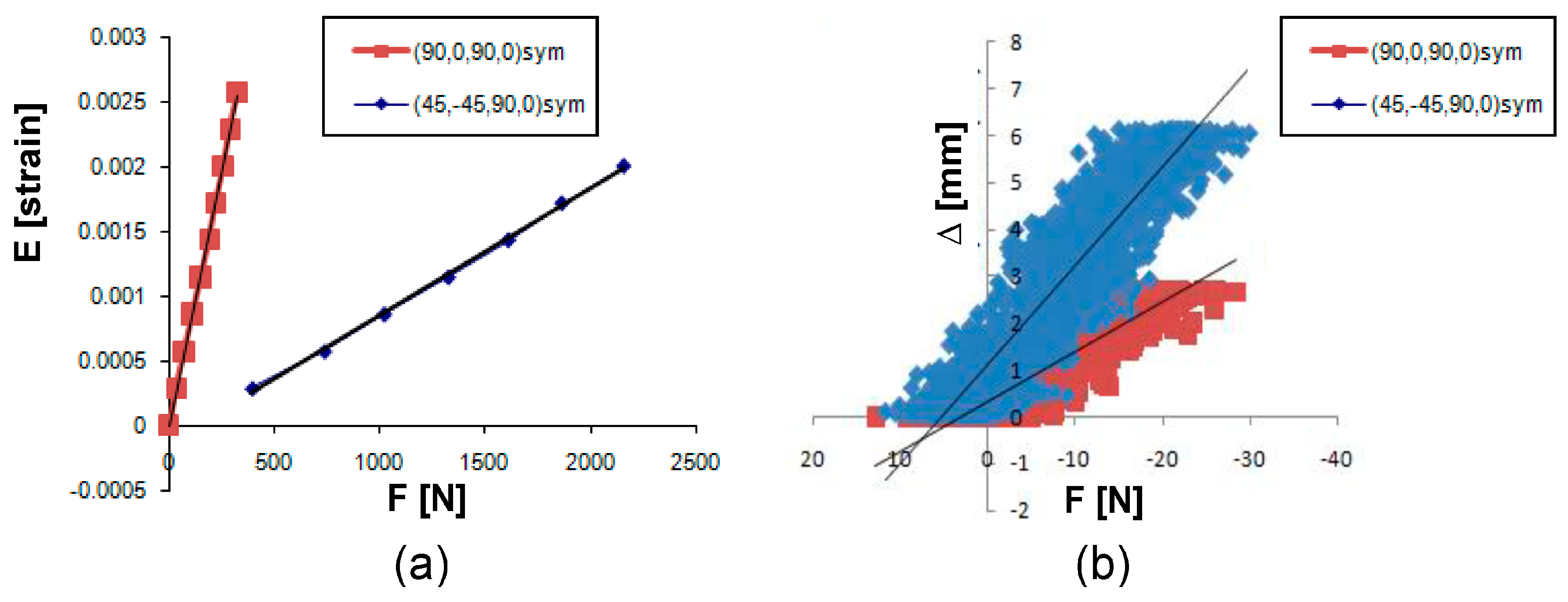
The wing’s flexibility creates an aeroelastic coupling between the wing’s geometrical formation and the aerodynamic forces generated by it. This aeroelastic problem was solved iteratively, by assuming a geometrical twist (a certain ${\alpha }_{tip}$ for a given ${\alpha }_{root}$), calculating the distributed lift force using rotary wing’s equation, applying the force on the wing using a finite element analysis, and correcting the geometrical twist according to the structural analysis results.

The various material properties used for calculation of the wing were based on test results performed on two rectangular specimens, produced by the same method as the wing. The specimens’ laminations were (45°, −45°, 90°, 0°)_sym and (90°, 0°,90°, 0°)_sym. The specimens were tested for tensile and bending and their results are presented in Figure 14.

Then a finite element (FE) model was generated for the rectangular specimens and loads similar to the ones used in the test campaign were applied on the FE model. The model properties were altered to produce similar results to the experiments’ within an error of up to 5% (see

Table 1. A comparison between the experiments results and the finite element analysis.

Load Type	Laminate	Model Properties			Load (N)	Displacement (mm)
		Ex (GPa)	Ey (GPa)	Gxy (GPa)		Test	FE	Error (%)
Bending	(45°, −45°,90°, 0°)sym	45	8.6	3.8	20	4.22	4.43	4.976
	(90°, 0°,90°, 0°)sym	45	8.6	3.8	20	2.14	2.15	0.467
Tensile	(45°, −45°,90°, 0°)sym	45	8.6	3.8	2000	0.40	0.38	5.000
	(90°, 0°,90°, 0°)sym	45	8.6	3.8	2000	0.32	0.31	3.125

).

The chosen parameters for the wing’s finite element model were therefore:

• $E_x=45(\text{GPa})$, Young’s modulus in the fiber direction;
• $E_y=8.6(\text{GPa})$, Young’s modulus perpendicular to the fiber;
• $G_{xy}=3.8(\text{GPa})$, shear modulus of the laminate;
• ${\gamma }_{xy}=0.32$, Poisson ratio.

4.2. Reynolds Numbers of the Tested Wings

The first wing to be tested was described in Section 2 and had a wing span of 1.1 m and a chord of 18.5 cm. Due to technical testing difficulties, encountered during the tests, the flapping frequency was limited to only 1.5 Hz, and not at 3 Hz as originally planned. The Reynolds number was then:

$${\left(\mathrm{Re}\right)}_{long-wing}=\frac{V\cdot L}{\nu }=\frac{\Omega r_2\cdot r_2}{\nu }=\frac{1.5\pi \cdot 1.1\cdot 1.1}{15.7\cdot {10}^{-6}}=30,000$$

(38)

Based on the test results for the first wing, our preliminary calculations were updated, and built a smaller wing, in order to attain a higher efficiency. The smaller wing had a wing span of 55 cm and a chord of 14 cm. It was flapped at 2.5 Hz and at Reynolds number of:

$${\left(\mathrm{Re}\right)}_{short-wing}=\frac{2.5\pi \cdot {0.55}^2}{15.7\cdot {10}^{-6}}=15,000$$

(39)

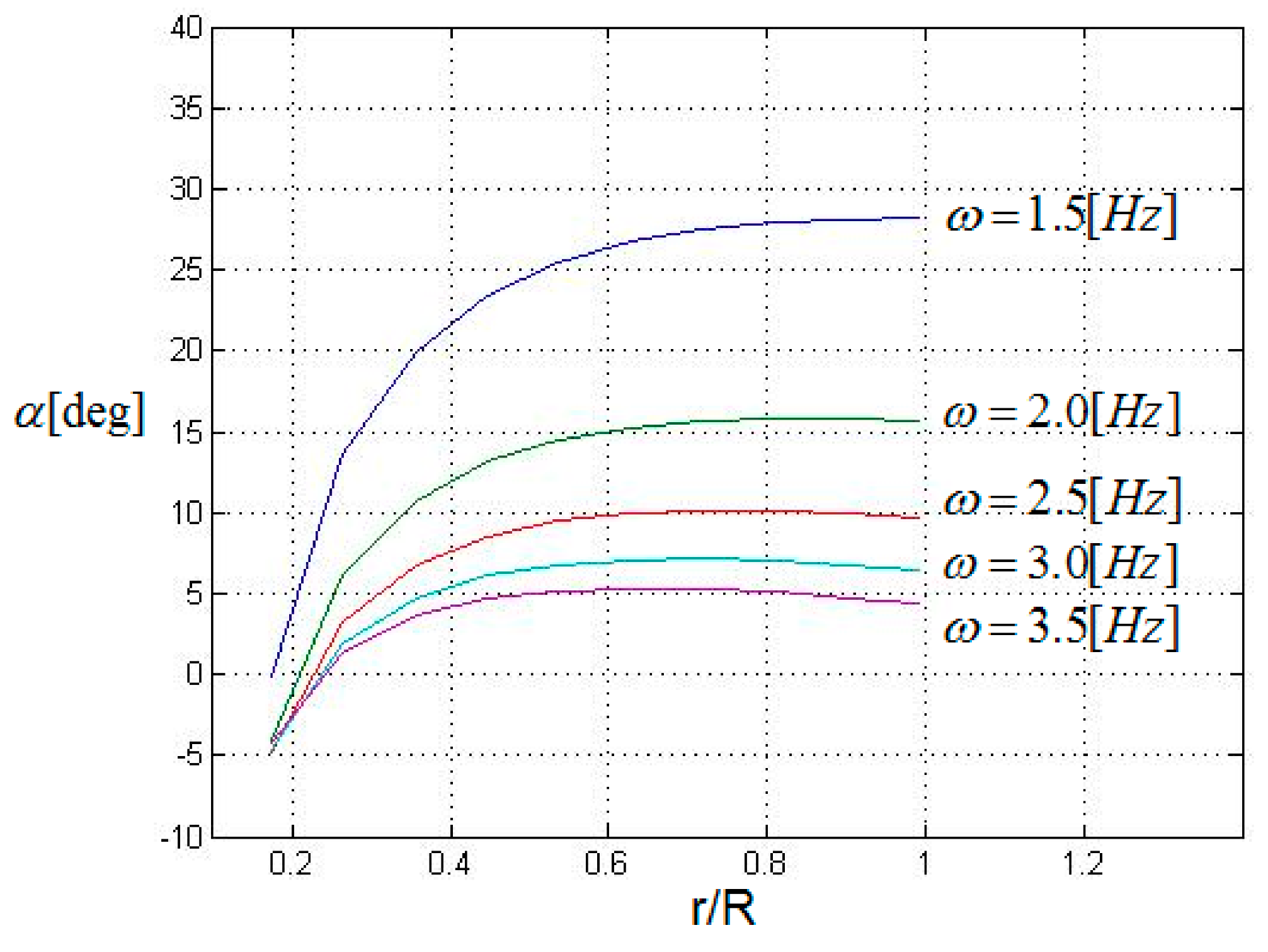
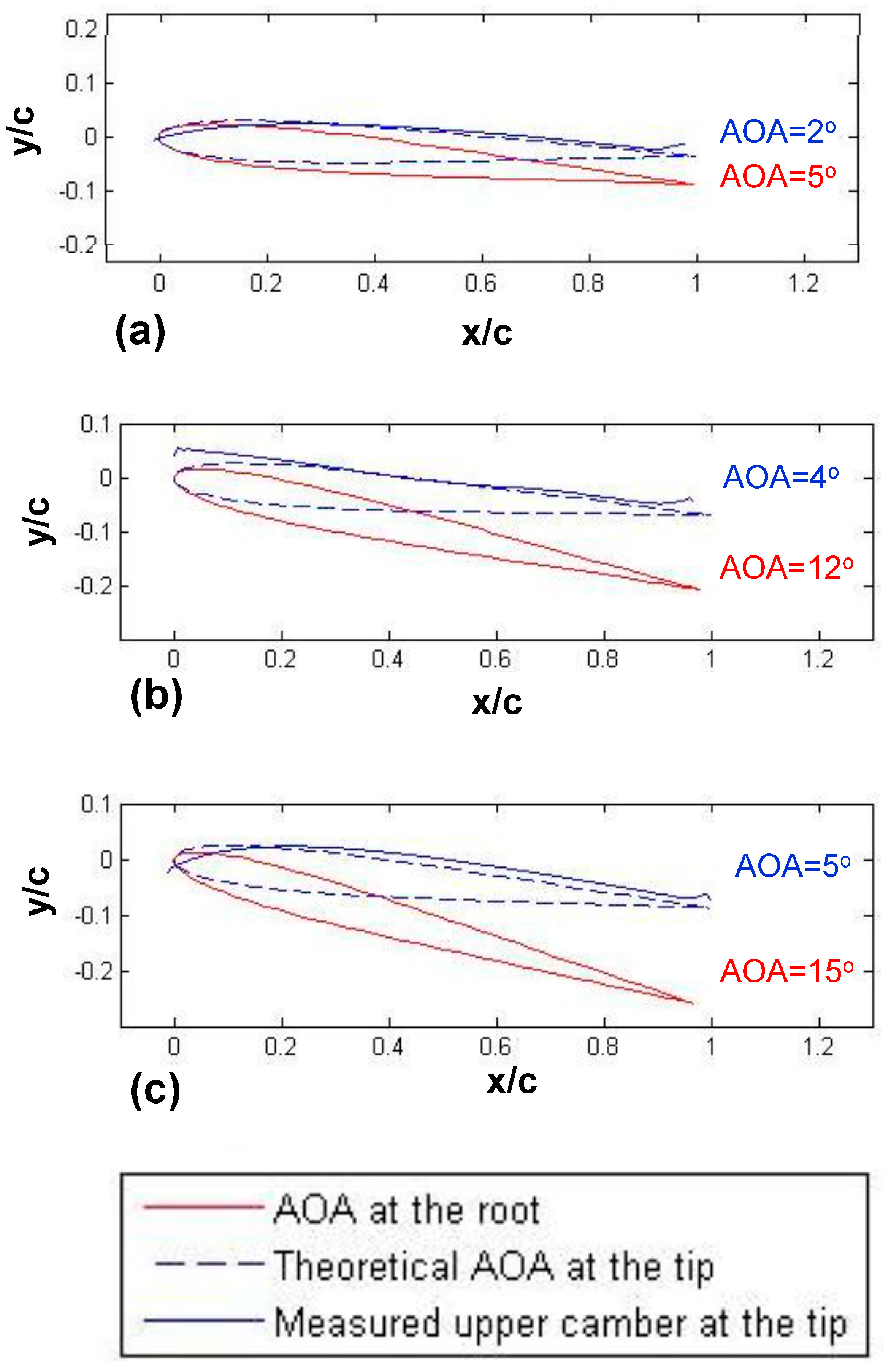
4.3. Torsion at the Wing Tip

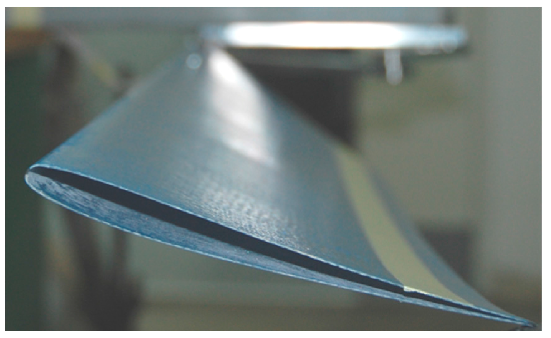
First, the laser rangefinder was placed above the wing tip at middle stroke, and the upper wing camber, was measured as a function of the AOA at the root. The measured results were compared to those obtained by the finite element analysis (see results in Figure 15). An image of the twisted wing is shown in Figure 16.

4.4. Moments at the Wing Root

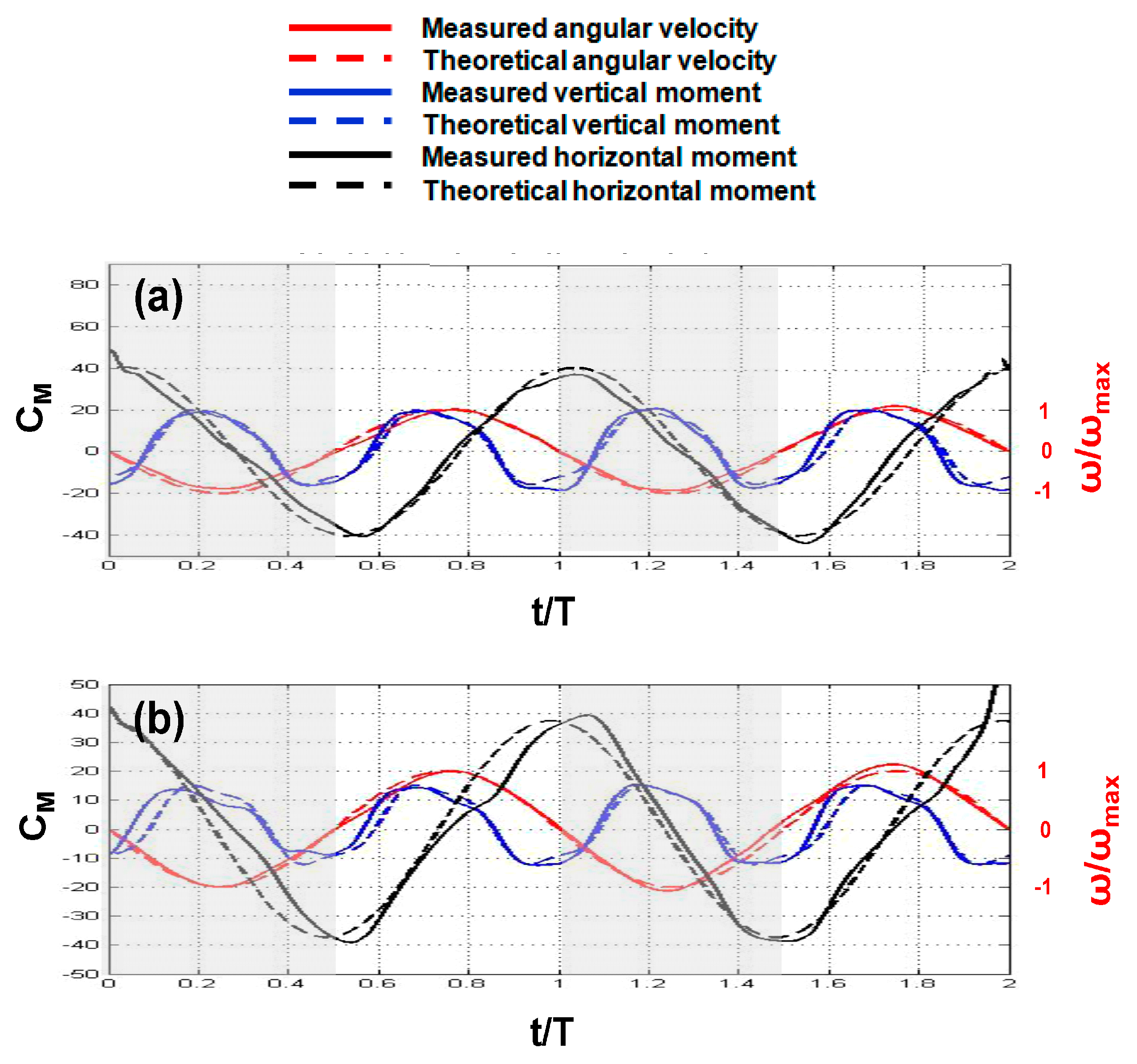
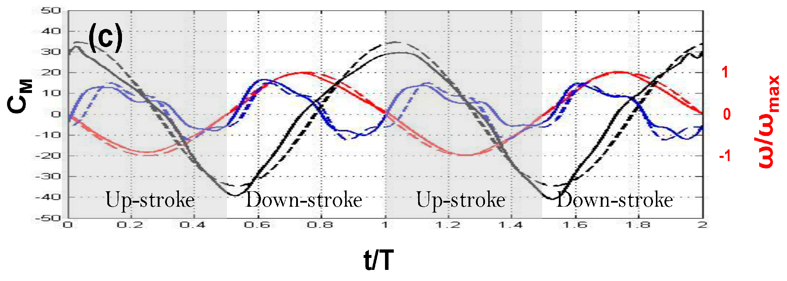
The vertical and in-plane bending moments at the root of the wing, were measured and compared it to the analytical solution described in subsections 3.2 and 3.3. The wing of 1.1m span and a chord length of 18.5 cm was flapped at a frequency of 1.5 Hz, at three angles of attack, as shown in Figure 17. The analytical solution was then corrected empirically, by minimizing the natural frequency of the wing ω_n by 0.68, and by adding a phase of 0.2π (phase delay) to match both solutions. The amplitude of the natural vibration (Equation (27)) was chosen to be C₁ = 0.005 and C₂ = 0, where C₁ and C₂ are the coefficients of the sine and cosine terms forming the response of the wing. The differences between the analytical calculations and the experimental results are due to the mathematical neglections that were made during the derivations of the equations. In Equation (27) in Section 3, the damping effect on the vertical movement of the wing was neglected, which in physical experiment acts to decrease the amplitude of flapping. This effect can be represented as a decrease in the natural frequency of the wing. In addition, the transition effects, which occur at the end of each flapping stroke were also neglected. These effects, such as clap-and-fling [7] and wake capture [44], may result in a phase delay.

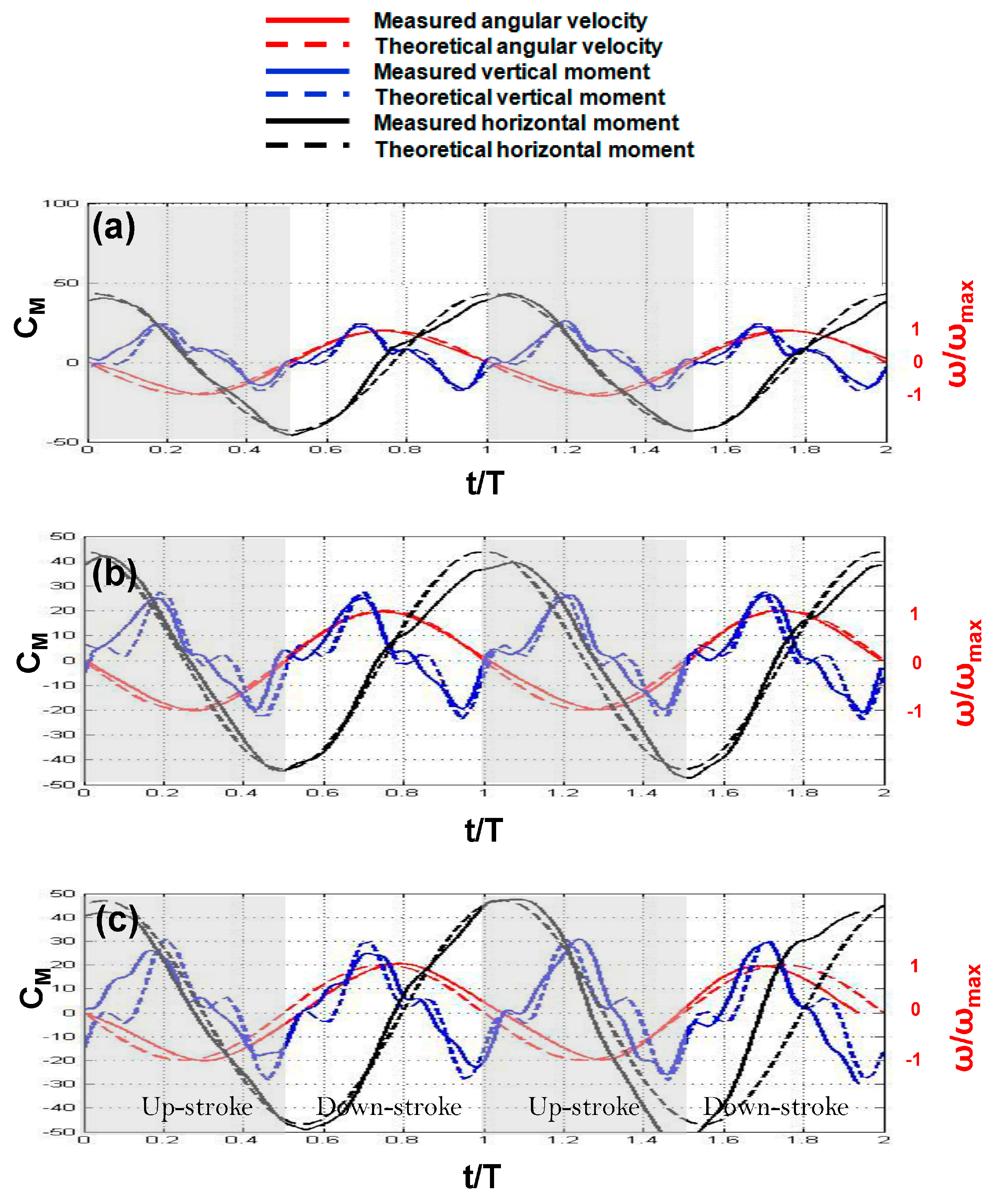
The improved mathematical model was validated through tests on a second wing, having a span of 55 cm and a chord length of 14 cm, at a flapping frequency of 2.5 Hz. A good agreement between the model predictions and the measured results (Figure 18) was found.

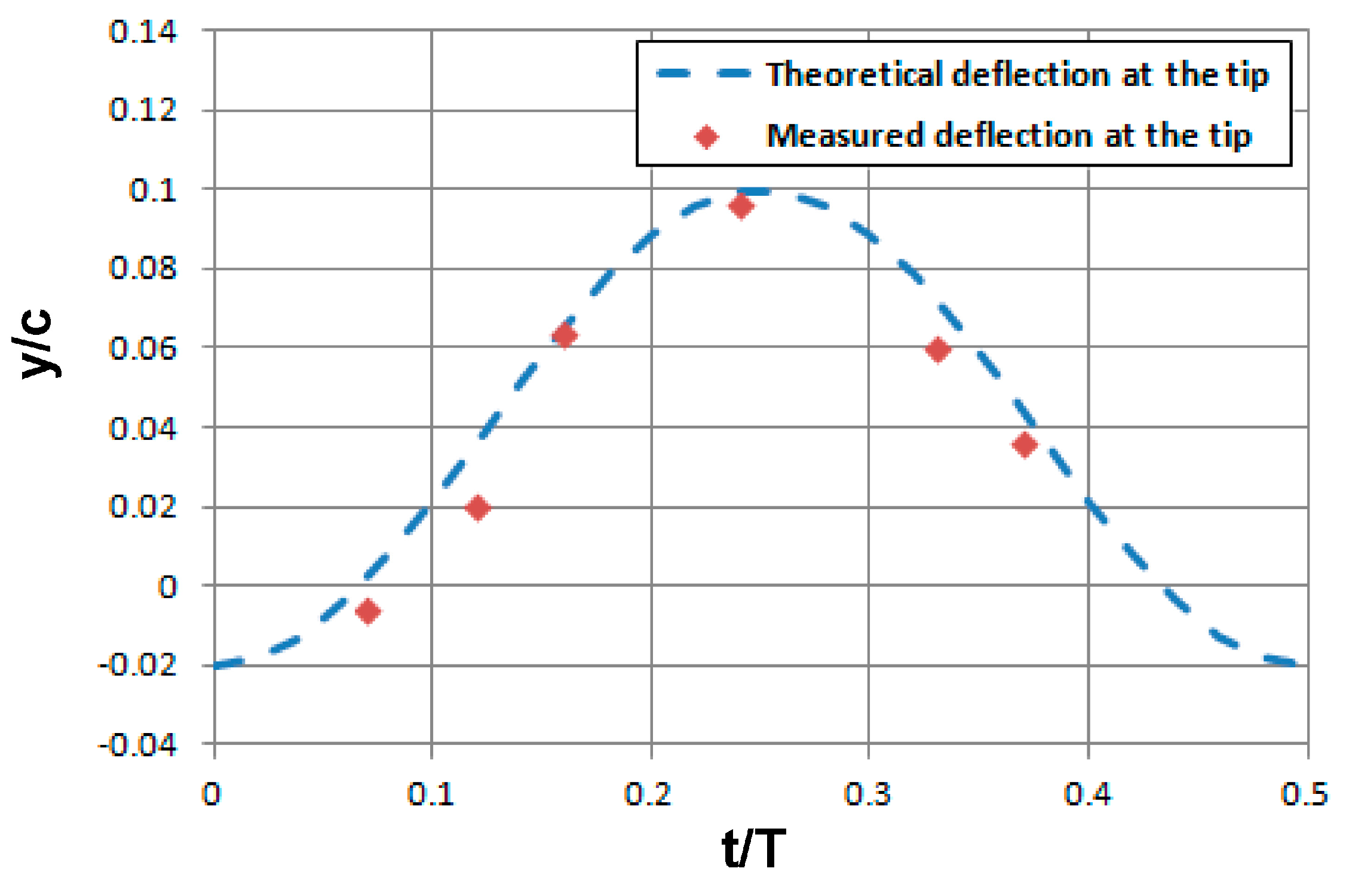
4.5. Vertical Displacement

Next, the laser rangefinder was placed at different locations along the flap stroke, and compared its vertical displacement of the wing tip to the relevant analytical solution, as shown in Figure 19, yielding a good matching.

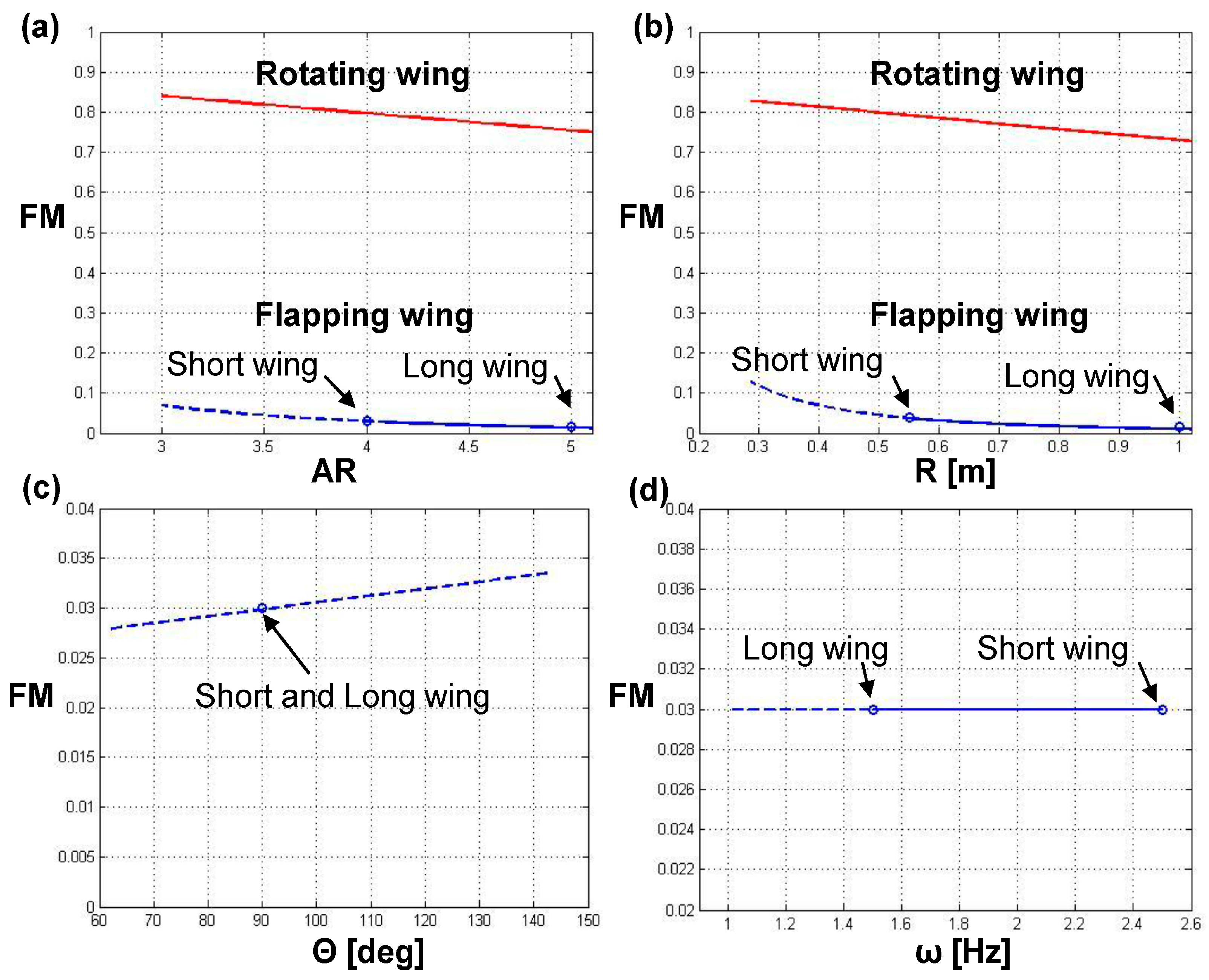
4.6. Hover Efficiency for Flapping Wings—The Figure of Merit

At the end of the study, the hover efficiency for the flapping wing, what it is also called the figure of merit (FM) was investigated. The present research suggested a flapping wing structure to propel a lightweight air vehicle. Then a simplified analytical model was developed aimed at “catching” the aerodynamic performances of the wing, and improved it empirically based on subsequent tests. The improved model, validated by a second set of measurements on a shorter wing, enabled the extrapolation beyond the envelope of the measurements. The figure of merit of the hovering flapping wing was investigated by examining the effect of wing span, aspect ratio, flapping frequency and stroke amplitude on it. To isolate the influence of each parameter, for each parameter calculation all the other parameters were set to be those of the long wing and evaluated the figure of merit of both wings with these parameters.

The figure of merit calculation method was adopted from helicopters aerodynamics [40]. It is the ratio between the ideal moment required to propel the rotor, and the actual moment. The ideal moment consists of the in-plane bending moment generated by the induced drag, and the actual moment as presented in Equation (40):

$$F{M}_{flapping}=\frac{M_{ideal}}{M_{actual}}=\frac{{\overline{M}}_{aerodynamic\_induced}}{{\overline{M}}_{aerodynamic\_parasite}+{\overline{M}}_{aerodynamic\_induced}+{\overline{M}}_{inertial}}$$

(40)

where the moments were defined in subsection 3.3, and are averaged over time as follows:

$$\overline{M}=\frac{\omega }{\pi }{\displaystyle \underset{0}{\overset{\frac{\pi }{\omega }}{\int }}M}\cdot dt$$

(41)

The lift force is reflected through the induced aerodynamic moment (Equation (33)).

The propelling efficiency of the flapping wing was compared to the efficiency of a rotating wing having similar characteristics (Equation (41)). In the rotating system, since the angular velocity is constant, there is no inertial moment, nor vertical movement of the wing. Therefore, only the inflow produces the induced AOA.

$$F{M}_{rotating}=\frac{M_{ideal}}{M_{actual}}=\frac{{\overline{M}}_{aerodynamic\_induced}}{{\overline{M}}_{aerodynamic\_parasite}+{\overline{M}}_{aerodynamic\_induced}}$$

(42)

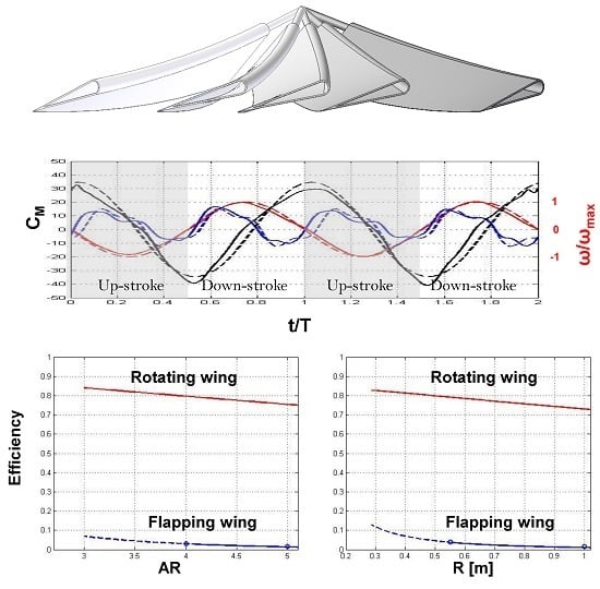
The results of the hovering efficiency for a rotating vs. flapping wing are presented in Figure 20a–d. In each figure one parameter was changed and all the other were set to be those of the long wing. An alteration of these fixed parameters within the experimental envelope (AOA—5° to 15°, Aspect Ratio—4 to 6, wing span—0.55 to 1.1 m, flapping frequency—1.5 to 2.5Hz) does not change qualitatively the curves plotted in Figure 20. As expected, the rotating wing has a much better efficiency than the flapping wing as a function of aspect ratio and wing span. When investigating the flapping wing, its efficiency is not influenced by the flapping angular frequency, however when increasing its stroke amplitude, the FM slightly increases.

In this study, the aerodynamic moments in the horizontal plane were negligible (less than 10%) compared to the inertial ones. However, the vertical aerodynamic moments, caused mainly by the lift force, were substantial, and constituted more than 90% of the total vertical moments. These vertical forces had a profound effect on the final efficiency.

5. Discussion, Conclusions and Further recommendations

In the present study an insect inspired flapping wing structure was designed based on simplified aerodynamic model, and the parameters affecting its performances were investigated. The focused parameters were: The wing span, the aspect ratio, the flapping frequency and the stroke amplitude. Each of these parameters might have implications on future design of flapping-winged MAVs.

5.1. The Wing Span Influence

As was expected, the propelling efficiency of the flapping wing, at the measured span (1.1 m span) was very poor, compared to that of the rotating one (Figure 20b). These poor performances are due to the high inertial moment required to accelerate and decelerate the flapping wing at each stroke. The wing’s mass is proportional to the third power of the wing's span (as other two dimensions, chord length and thickness are given as percentage of the wing’s span); therefore propelling using flapping wings becomes more efficient only at micro air vehicles (wing span less than 15 cm). Although the model predicts high efficiency at small wing spans, it should be validated through experiment, since there are other phenomena that were not significant at our wing span. Additionally, flapping winged flyers enhance their efficiency by elastically storing the energy required to accelerate and decelerate the wing, by flapping at the resonance frequency of the spring–mass system [25]. Therefore such kinetic energy storing for future design of MAV, is recommendable. To implement this idea, a torsion spring should be placed at the wing’s root, and the spring’s rate should be designed to fit the wing’s mass and the desired flapping frequency.

5.2. Wing Aspect Ratio Influence

Unlike stationary wings, the present model predicts that a smaller aspect ratio will increase the propelling efficiency of the flapping wing (Figure 20a). A slender wing has a large moment of inertia around the root, and consequently requires more power to accelerate. The study of Usherwood and Ellington [19], which showed that the wing’s aspect ratio has little effect on the force coefficients, obviously did not take in consideration the inertial forces applied on the wing. This property of flapping wings should be taken into account in the design of future flapping-winged MAV.

5.3. Wing Flapping Frequency and Stroke Amplitude Influences

Based on the model developed and tested in the present study, the wing flapping frequency has no effect on the propelling efficiency (Figure 20d), assuming that the flow is inviscid, incompressible and non-rotational. On the other hand, an enhancement of the flapping stroke amplitude improves the propelling efficiency (Figure 20c), namely, for the same inertial moment more lift is produced. A similar conclusion can be derived by reanalyzing the data of Meng et al. [28] who calculated the aerodynamic forces generated by a corrugated flapping wing. In their study, the lift to drag ratio increases as the stroke amplitude increases, for all corrugated wing models. Insects, such as bees, beetles and dragonflies [24], have stroke amplitudes of about 150°, presumably for this reason. Most studies to date, investigating flapping wings, use a four-bar linkage flapping mechanisms [14,16,17,45]. Using this type of mechanism makes it technically difficult to achieve amplitudes larger than 90°. Our study suggests that future development in the field would require the design of an alternative flapping mechanism capable of achieving stroke amplitudes larger than 90°.