1. Introduction
Optimization is the process of finding the best solution from a set of available alternatives, taking into account all of the required problem constraints [
1]. A single objective optimization problem consists of finding the minimum or the maximum value of an objective function that measures the quality of each solution. The variables of optimization problems can be either continuous or discrete. Optimization problems with discrete variables are also called combinatorial optimization problems [
1], and the examination timetabling problem (ETP) that is solved in this work belongs to this class of problems.
There are many techniques and algorithmic strategies that are used to solve difficult combinatorial optimization problems, but none of them manages to solve efficiently all of the categories of optimization problems, as Wolpert and Macready [
2] proved. Mathematical programming [
3], artificial intelligence [
4] and meta-heuristic techniques [
5] are some of the algorithmic families for the solution of these problems. The class of evolutionary algorithms (EA) [
6,
7,
8], which is used in this paper, is based on Darwinian theory [
9] and is usually included in the computational intelligence family.
The examination timetabling problem (ETP) is a problem of great importance for every University, as it implicitly affects the performance of students in examinations. The goal is to assign a set of examinations to a set of time slots in a way such that a set of constraints are satisfied. Some constraints are hard and should not be violated, as a student should not have to sit for two exams at the same time, while others are soft, and violating them results in a bad solution. Practical aspects of the ETP problem can be found in [
10] alongside an approach of solving the problem carried out by our team in [
11]. There is a rich literature on the ETP, including benchmark datasets, as the ones used in this work, proposed by Carter [
12], with a simplified version of the problem. Other known benchmarks available are the University of Nottingham benchmark data [
13] and the University of Melbourne benchmark data [
14].
Parallel computation has gained significant interest in recent years due to the fact that the computer clock speed cannot be increased anymore, due to the physical limitations of semiconductor technology [
15]. In order to sustain the constant increase of processing power, manufacturers promoted the multicore and many-core architectures. Graphical processing units (GPUs) are powerful commodity computer components that include a large number of processing cores in order to provide better performance of computer graphics. However, given the available processing power, GPU processors attracted the interest of many researchers and scientists for generic computation, as well, leading to the introduction of the term, general purpose graphical processing units (GPGPUs). After NVIDIA introduced the Compute Unified Device Architecture (CUDA), a large number of scientific applications have been ported to GPUs with remarkable speedups [
16,
17].
In this paper, a hybrid evolutionary algorithm (hEA) is presented that is designed to solve the ETP using a GPU. The computing power of the GPU gives the opportunity to explore better the solution space by using great population sizes. Emphasis is given to the encoding and the representation of the solution in order to take full advantage of the GPU architecture. Moreover, the compressed sparse row format is used for the conflict matrix to improve performance, while a greedy steepest descent algorithm component is employed to improve the quality of the solutions of the genetic algorithm in every generation. Furthermore, the significance of the size of the tournament selection as the population size grows is shown.
In the next section, the problem description is stated. In
Section 3, related work for the ETP problem is surveyed, while in
Section 4, an introduction to the GPU architecture and the CUDA programming model is presented. Our design approach for the ETP is described in the next section, and
Section 6 shows the results of the experiments undertaken. In the final section, conclusions and some future directions are proposed.
2. Problem Description
The examination timetabling problem (ETP) is an optimization problem, whose goal is to assign a set of examinations to a set of time slots in a way that a set of constraints are satisfied. The constraints are categorized as hard for the ones that should be satisfied in order for a timetable solution to be feasible and legal and soft for the ones for which when satisfied, the solution becomes better in terms of quality. Two versions of the ETP problem exist, the capacitated and the uncapacitated one. In the capacitated version, the room capacity is taken into account, while in the uncapacitated, it is not. In this paper, the Carter/Toronto datasets are used as benchmarks to evaluate the proposed algorithm. For these datasets, there exists essentially one hard constraint that has to do with the fact that a student cannot sit in two or more examinations at the same time. The main soft constraint involves the spreading of the examinations in the whole examination period in order to facilitate the preparation of the students. The Carter/Toronto benchmark Version I problems are summarized in
Table 1.
Table 1.
Toronto examination timetabling problem (ETP) datasets.
Table 1.
Toronto examination timetabling problem (ETP) datasets.
| Dataset | Examinations | Students | Periods | Conflict Density |
|---|
| car-f-92 I | 543 | 18,419 | 32 | 0.14 |
| car-s-91 I | 682 | 16,925 | 35 | 0.13 |
| ear-f-83 I | 190 | 1125 | 24 | 0.27 |
| hec-s-92 I | 81 | 2823 | 18 | 0.42 |
| kfu-s-93 I | 461 | 5349 | 20 | 0.06 |
| lse-f-91 I | 381 | 2726 | 18 | 0.06 |
| pur-s-93 I | 2419 | 30,032 | 42 | 0.03 |
| rye-s-93 I | 486 | 11,483 | 23 | 0.07 |
| sta-f-83 I | 139 | 611 | 13 | 0.14 |
| tre-s-92 I | 261 | 4360 | 23 | 0.18 |
| uta-s-92 I | 622 | 21,266 | 35 | 0.13 |
| ute-s-92 I | 184 | 2749 | 10 | 0.08 |
| yor-f-83 I | 181 | 941 | 21 | 0.29 |
A formal description of the problem follows. Let
E be a set of examinations assuming values one to
and
P a set of periods assuming values one to
. Binary variables
are defined over each
and
assuming value one if exam
i is scheduled to period
p or zero otherwise. Let
S be the total number of students,
be the number of students that examinations
i and
j have in common and
w a weight vector that assumes values
. Each of the
w’s values corresponds to a distance between two examination periods. When the distance between two examinations is only one time slot, the value of
w is 16, and as the distance increases, the value of
w decreases. Equation (
1) is the objective function that should be minimized. Constraint Equation (
2) ensures that each exam will be assigned to exactly one period. Constraint Equation (
3) assigns to variables
the number value of the period to which examination
i is scheduled. Constraint Equation (
4) ensures that no two examinations having students in common will be scheduled to the same period. In this constraint,
M is a very large number and
is the distance between the time slots to which examinations
i and
j are scheduled.
s.t.
For this problem, a conflict matrix that shows the percentage of examinations with common students among the various examinations and, in effect, models the computational complexity of the problem is also defined. The (
) conflict matrix, with the examinations being both on its rows and columns, has the value “1” at the intersections of pairs of examinations with common students between them. Furthermore, the conflict density parameter in
Table 1 is the number of elements with value “1” in the conflict matrix divided by the total number of elements of the matrix.
3. Related Work
Many approaches have been published to tackle the ETP problem, and there are various surveys that examine them. Qu
et al. [
18] published a very thorough survey describing the problem, the techniques used to solve it and the benchmark datasets that exist for this problem, while Schaerf [
19] presents the approaches published to solve the school timetabling problem, the university course timetabling problem and the examination timetabling problem. Furthermore, in Petrovic and Burke [
20], the integration of several approaches about university timetabling problems aiming at achieving a higher level of generality is discussed. According to Qu
et al. [
18], the techniques used to solve the ETP problem can be categorized into graph based, constraint based, local search based, population based, multi-criteria techniques and hyper-heuristics.
In the graph-based techniques category belongs the work of Welsh and Powell [
21], which is very important, as they show the relation between graph coloring and timetabling. Carter
et al. [
12] examine the impact of six ordering heuristics in timetabling problems. The heuristics examined are saturation degree, largest degree, largest weighted degree, largest enrollment, random ordering and color degree. Moreover, in this work, the 13 Toronto datasets have been introduced, which have been a performance benchmark for most ETP research since. Asmuni
et al. [
22] use fuzzy logic for the solution of the ETP problem, while Corr
et al. [
23] developed a neural network to decide the difficulty of an examination to be scheduled according to more than one ordering heuristics. Furthermore, Burke and Newall [
24] solve the ETP problem with a more general and faster method by adapting heuristic orderings. This method was examined in many benchmark problems and proved to be a robust and reliable solution.
Another category of techniques that were applied to the ETP problem is the constrained-based techniques. Brailsford
et al. [
25] show how combinatorial optimization problems can be solved using these techniques. In the same category falls the work of Merlot
et al. [
14] given that they use a constrained programming method to create initial solutions in the first phase. However, in a second phase, simulated annealing and hill climbing, which belong to local search methods, are applied in order to improve the solutions.
Local search-based techniques include hill climbing, simulated annealing and tabu search. Gaspero and Schaerf [
26] use a combination of two tabu search-based solvers in order to solve the ETP problem, one to focus on the hard constraints, while the other to provide other possible improvements. White
et al. [
27] show that long-term memory can improve tabu search to a great extent. Casey and Thompson [
28] designed a greedy randomized adaptive search procedure (GRASP) algorithm, where in the first greedy phase, a feasible, collision-free timetable is constructed, and in the second, the solution quality is improved. Duong and Lam [
29] present a solution that uses the backtracking with a forward checking algorithm to create an initial legal solution and simulated annealing to improve the cost of the solution. Caramia
et al. [
30] use local search techniques to obtain some of the best available results in the bibliography, while Thompson and Dowsland [
31] designed a robust system, which solves the ETP problem with a simulated annealing algorithm.
Another widely-used technique uses population-based algorithms, such as genetic, memetic and ant algorithms. Burke and Silva [
32] in their survey discuss the decisions that should be taken into account in order to design an effective memetic algorithm and particularly examine the infeasibility of the solutions as part of the search space, the fitness evaluation function with the complete and approximate evaluator, the encodings of the algorithm, the fitness landscape and the fraction of the algorithm that should be done with the genetic operators and the fraction that should be done with local search. Moreover, Burke and Newall [
33] designed a memetic algorithm, the main contribution of which is that it splits the problem into subproblems, so that the computational time decreases and the quality of the solutions increases. Eley [
34] present a Max-Min ant system to solve the ETP. In their work, Côté
et al. [
35] solve the same problem with an evolutionary algorithm that, instead of recombination operators, uses two local search operators. Furthermore, Burke
et al. [
13] present a memetic algorithm with two mutation operators followed by hill climbing techniques. No crossover operator is used. Another approach is described by Erben [
36], who attacks the ETP problem with a grouping genetic algorithm giving emphasis to the encoding and the fitness function to obtain good quality solutions. A different solution strategy is proposed by Deris
et al. [
37], who combine the constraint-based reasoning technique with a genetic algorithm (GA) to find good quality results. The informed genetic algorithm designed by Pillay and Banzhaf [
38] consists of two phases, with the first focusing on the hard constraints and the second on the soft constraints.
Apart from the above-mentioned techniques, a number of solution approaches originating from various disciplines have been proposed, and satisfactory results were reported with various metaheuristics [
39], hyper heuristics [
40,
41], hybrid methods [
42] and others.
There are also many works dealing with parallel metaheuristics. Alba
et al. [
43] conducted a thorough survey about parallel metaheuristics, both trajectory based and population based. They examine many of the applications that parallel metaheuristics apply, the programming models, the available parallel architectures and technologies, as well as the existing software and frameworks. Lazarova and Borovska [
44] present a comparison of a parallel computational model of ant colony optimization of simulated annealing and of a genetic algorithm applied to the travelling salesman person problem. Talbi
et al. [
45] examine parallel models for metaheuristics, such as self-contained parallel cooperation, problem-independent and problem-dependent intra-algorithm parallelization. They analyze the calculation time and surveyed many works for the specific models. Recently, extended research has been done in porting GAs to GPUs. Pospichal
et al. [
16] designed an island model for a genetic algorithm in CUDA software and tested it with some benchmark functions. All of the parts of the algorithm are executed in the GPU, and the results show a speedup of about 7,000× compared to a CPU single-threaded implementation. Moreover, Maitre
et al. [
46] present a genetic algorithm that evaluates its population in the GPU with a speedup of up to 105×. Wong [
47] built a multi-objective evolutionary algorithm in a GPU with a speedup between 5.62 and 10.75. A different approach is given by Luong
et al. [
48]. A hybrid genetic algorithm is shown, and only the generation and the evaluation of the neighborhood of the local search procedure are done in parallel, with a speedup up to 14.6×. Furthermore, a fine-grained parallel genetic algorithm is described in Yu
et al. [
49] achieving a speedup of about 20.1×. A hierarchical parallel genetic algorithm is presented by Zhang and He [
50], but no experimental results are shown. Vidal and Alba [
51] described a cellular genetic algorithm with the complete algorithm running on the GPU, and the speedup is up to 24×. A CUDA implementation of a parallel GA, both binary and real coded, is described in Arora
et al. [
17] with very good speedups, up to 400×. They propose modifications, not only in the evaluation function, but also in the genetic operators.
To our knowledge, there is no previous work solving the examination timetabling problem with a hybrid evolutionary algorithm on a GPU. In this paper, such an algorithm is proposed, and tests have been made in order to evaluate its performance. Our goal is to achieve the best possible speedup, but also to obtain comparable quality solutions with the already published ones. The encoding that, according to our study, matches the GPU architecture better, is chosen, and although the datasets used do not have many constraints, the experimental results promise good performance for more constraint timetabling problems.
4. The GPU Architecture and CUDA Programming Model
Before going into detail on the design options, a description of the GPU architecture and the CUDA programming model is given. The details of the programming model given below apply to the Fermi architecture of graphics cards, such as the ones used in this work. GPUs are powerful and relatively cheap parallel machines, whose initial goal was the improvement of graphics processing. Due to their high computational power, they attracted the interest of many scientists and researchers, who tried to harness the power of GPUs in order to boost the performance of their scientific applications. The first attempts to program GPUs were with the use of OpenGL. Given that many researchers used GPUs for applications other than graphics, NVIDIA introduced in 2007 the Compute Unified Device Architecture (CUDA) in order to make GPUs more friendly to programmers not familiar with graphics. The language used is an extension to the C programming language. After the introduction of CUDA, the use of GPUs was increased significantly. Many papers have been written since then, reviewing the speedups achieved and the new capabilities GPUs give in the solution of scientific problems [
52]. Apart from CUDA, OpenCL is a standard that is becoming popular and is about parallel programming in general. However, at the time of writing, CUDA is more widespread, and therefore, it was our choice for writing our algorithms.
Many works have been done that investigate how to get the best performance on the GPU [
53,
54,
55], including one of our team’s [
56]. In order to obtain the best performance of a GPU, its architecture should be taken into account, and some limitations should be overcome. GPUs need a large number of threads to be executed to be well utilized and to hide the memory latency. Threads are organized into groups of threads, called blocks of threads, and blocks are organized into grids. Each block contains a three-dimension array of threads, and each grid contains a three-dimension array of blocks. Every GPU has a number of streaming multiprocessors (SM), each one containing a specific number of CUDA cores, which is related to the generation and the model of the graphics unit. All of the cores inside a multiprocessor execute the same command, while cores in different multiprocessors can execute different commands. The part of the code that is executed on the GPU is called a kernel. The programmer is responsible for defining the threads each kernel should execute, and the GPU is responsible for allocating them to its resources. A kernel can have many blocks of threads, each one containing up to 1024 threads. A single block is executed on one multiprocessor. A multiprocessor can execute up to 1536 threads and up to eight blocks simultaneously.
Regarding the memory hierarchy, GPUs have a global memory that is relatively slow, but with a high capacity, a shared memory, located in every multiprocessor, which is many times faster, but with only up to 48 KB of space available, and a number of registers that are even faster. All of the threads have access to the global memory, while in the shared memory, only the threads of a block that is executed in the same multiprocessor can have access. The registers store the local variables of each thread.
It is of great importance to have many active threads during the execution of the kernel and to find the best configuration of threads per block and blocks per grid in order to achieve the best performance. Furthermore, the transfers to and from the GPU are time consuming; thus, they should be avoided as far as this is possible. Another important aspect in order to obtain the best performance in the GPU is trying to avoid the divergent execution of the threads within a warp. A warp is the number of active threads in a multiprocessor, which is equal to 32. The reason for this is that every thread would execute a different block of commands, depending on the validity of the condition imposed, and given that all threads of a warp should execute the same instruction in every time unit, some threads may be active, while the others wait, decreasing the performance. Another interesting point for best performance is the global memory access pattern. In GPUs, if a memory access pattern is coalescable, meaning that threads access contiguous memory locations, the number of necessary memory transactions decreases; thus, the performance increases. On the other side, if the memory access pattern is strided, the performance drops, and even worse, when the access pattern becomes random, then the performance is bad.
5. Methodology
In this work, a hybrid evolutionary algorithm is employed in order to solve the ETP problem. Firstly, a pool of initial solutions is created, and then, a genetic algorithm is applied. The evaluation of the solutions takes place and a new generation is created by applying a crossover operator and a mutation operator. Afterwards, a greedy steepest descent algorithm is employed to further improve the quality of the solutions. Given that the transfers of the data to and from the GPU are time consuming, the whole algorithm is executed on the GPU, except for the construction of the initial solutions, which, for now, is executed on the CPU of the host server and is considered as a pre-processing step.
5.1. Encoding and Representation
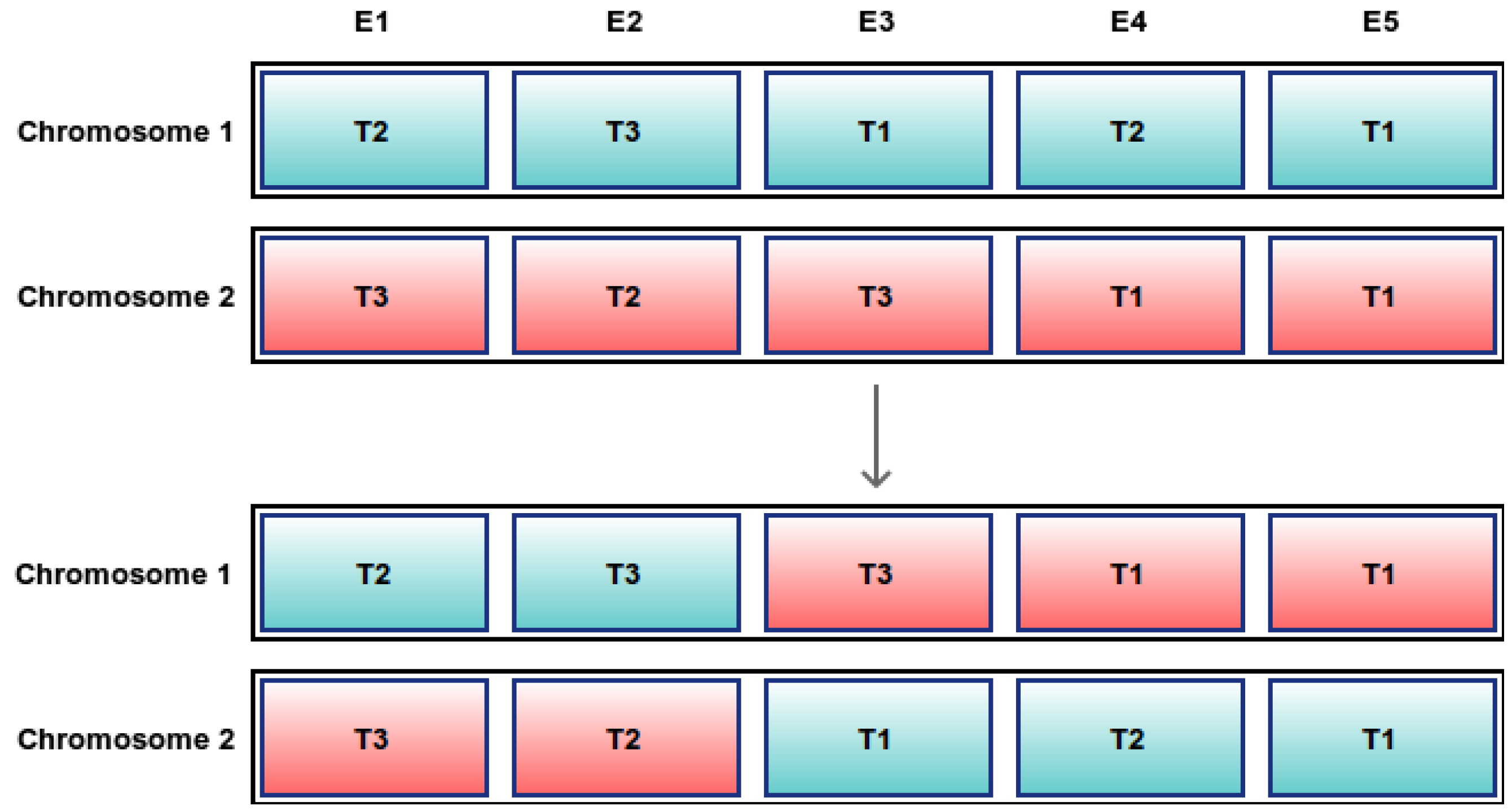
The selection of the encoding of the chromosomes is of great importance, as it affects the performance of the algorithm in terms of the speed and quality of solutions. The main encoding schemes are the direct and indirect encoding, also referred to as permutation and value encoding, respectively. In direct encoding, the chromosome is an array of integers with a size equal to the number of examinations, so that each cell corresponds to the respective examination, and the values of each cell of the array being the time slot in which the corresponding examination is scheduled (
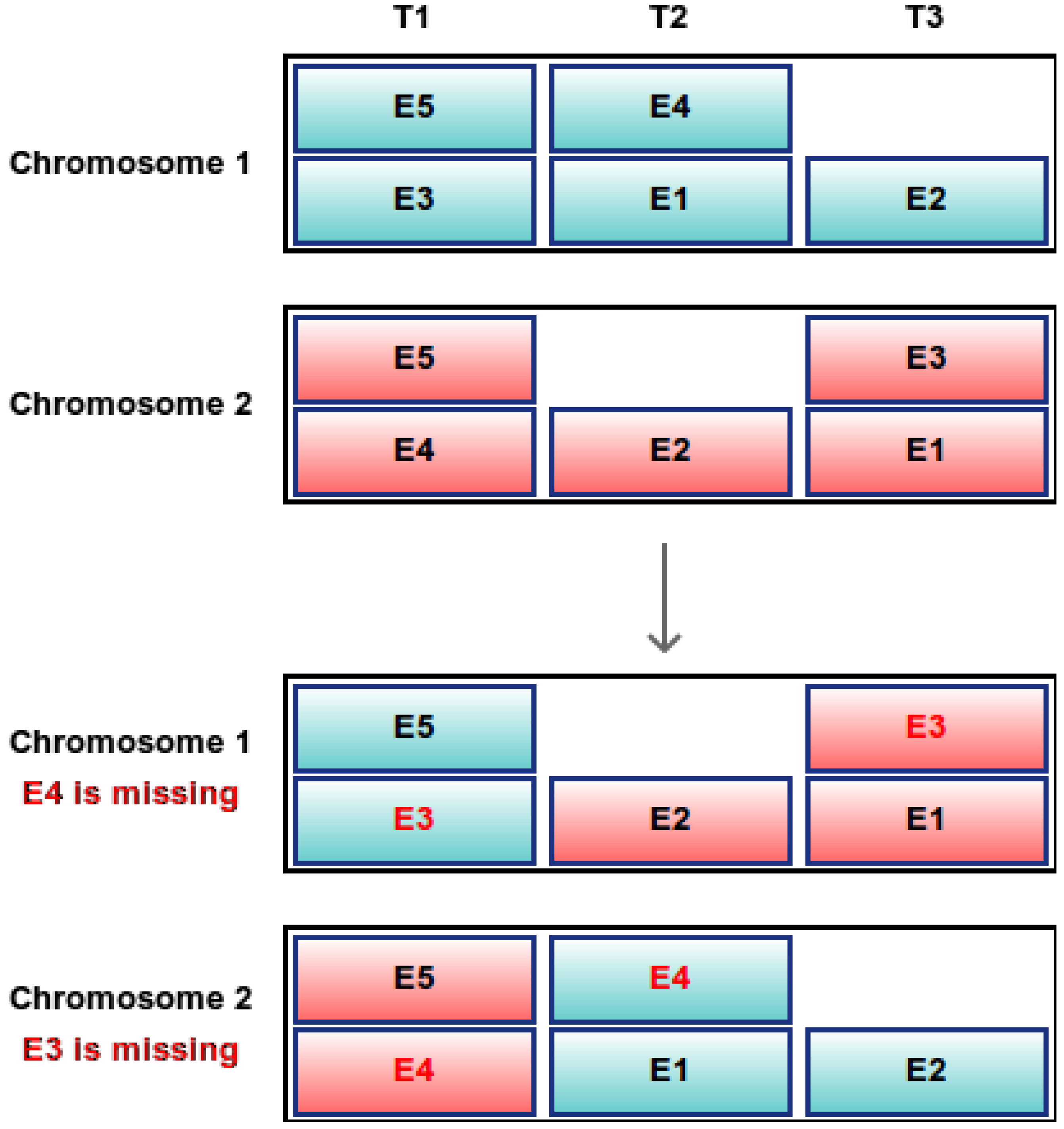
Figure 1). In indirect encoding, the chromosome is an array of lists of a size equal to the number of time slots. Thus, there exists one cell for every time slot, and each cell of the array contains the examinations that are assigned to the particular time slot (
Figure 2). Ross
et al. [
57] argue about the importance of the right chromosome encoding used in the algorithm and propose the cataclysmic adaptive mutation as a solution to the problems that direct representation introduces in the search process. In this work, the direct encoding scheme was selected, because the arrays are more suitable for the GPU vector architecture than the lists needed in the indirect encoding. In addition, the crossover operator in indirect encoding sometimes results in infeasible solutions, because some examinations may disappear or appear twice, as
Figure 2 shows (in bold red color, the examinations that appear twice are shown), while in direct encoding, this cannot happen (
Figure 1). In indirect encoding, if after the crossover operator, an examination is listed twice or not at all, usually a repair method is applied to find a similar legal solution.
Figure 1.
Direct encoding: single-point crossover between two chromosomes after the second gene. E1–E5: examinations; T1–T3: timeslots.
Figure 1.
Direct encoding: single-point crossover between two chromosomes after the second gene. E1–E5: examinations; T1–T3: timeslots.
Figure 2.
Indirect encoding: single-point crossover between two chromosomes after the first gene. Examinations in bold red are missing or appear twice. E1–E5: examinations; T1–T3: timeslots.
Figure 2.
Indirect encoding: single-point crossover between two chromosomes after the first gene. Examinations in bold red are missing or appear twice. E1–E5: examinations; T1–T3: timeslots.
5.2. Initial Construction of Solutions
The process of finding quality initial solutions is done at the CPU side as a pre-processing step. The starting population consists of a pool of algorithmically-computed solutions and a set of randomly-created solutions. The algorithmically computed solutions are very few in number (less than 250), and for their construction, the following approach is used. Examinations are ordered according to their largest degree (LD) values, which in effect brings the examinations with the most conflicts on top, and in each step, a specific examination is selected using roulette selection [
58] of the 20 or less still unscheduled examinations giving preference to higher LD values. Then, a period is selected randomly from the periods that do not already have examinations in conflict with the selected examination. If no such period exists, then a period has to be selected in which offending examinations should be removed before placement of the newly selected examination. This occurs by exploiting an extra field (removals) that tracks the removals of examinations that each examination is responsible for during the process of solution construction. Therefore, when an examination supersedes other examinations, the number of dislocated examinations is added to the removal field of the examination to be inserted. In order for the process of solution construction to progress, a period is selected based on the aggregate value of the removals field of all examinations that have to be removed and belong to this period. The basic idea is that the dislocation of examinations with a great total value of removals should be discouraged. This is achieved by organizing a tournament between periods that should be relieved from certain examinations where periods having a high removal value due to the examinations that are scheduled in them tend not to be selected. Algorithm 1 shows the pseudocode of this process.
| Algorithm 1: Construction of the initial solutions. |
![Algorithms 07 00295 i001]() |
5.3. Evaluation
The evaluator is based on Equation (
1). The division with
S is dropped, since
S is a scaling factor that does not add at all to the solution approach, while by omitting it, the computations are fully based on integer arithmetic instead of slower floating point arithmetic. Equation (
1) has to be calculated for all of the members of the population. The cost evaluation of every member is independent of the computation of the other members. For every examination indexed
i in the input, only the conflicts with examinations indexed
need to be considered. At this point, two independent processes are detected in order to be parallelized: the calculation of the cost of a whole chromosome and the calculation of the cost of a single examination. Both approaches were implemented. From now on, the first approach will be referred to as the chromosome-threaded approach, while the second will be referred to as the examination-threaded approach.
In the chromosome-threaded approach, each thread calculates the sum of a whole chromosome; thus threads are executed, where is the population size, and no synchronization is needed. Every thread computes the cost of the chromosome in a local variable, and at the end, it stores it in the global memory. The pseudocode for the chromosome-threaded approach is given in Algorithm 2.
| Algorithm 2: Evaluation, chromosome-threaded approach: each thread evaluates one chromosome of the population. |
![Algorithms 07 00295 i002]() |
In the examination-threaded approach, each thread calculates the cost of one examination only and places the result in an array in the shared memory. After the calculation of the cost of each examination, the total cost of the chromosome should be computed. The total cost of each chromosome can be computed with a reduction operation, keeping as many threads as possible active [
59]. After examining the characteristics of the datasets that are used in this paper, a problem occurs with the
pur-s-93 dataset. The number of examinations in this dataset is 2419, which means that 2419 threads are needed for the calculation of a single chromosome. However, due to the limitations of the CUDA programming model, each block can have up to 1024 threads, thus needing three blocks of threads if each block is configured to contain the most available threads. However, having a block with 1024 threads means that in that multiprocessor, only one block can be executed at the same time, since a multiprocessor can have up to 1536 threads, and therefore, the multiprocessor is not fully utilized. Taking these into consideration, our approach for the number of threads per block and the number of blocks is:
| Algorithm 3: Evaluation, examination-threaded approach: each thread evaluates one gene of the population. |
![Algorithms 07 00295 i003]() |
In the above equations, is the number of threads per block in the x direction, and are the number of blocks in the x and y direction, E is the number of examinations and is the population size. As can be seen from the above equations, we chose to split the work into two blocks of threads for all of the big datasets containing more than 512 examinations, and not only for the pur-s-93 dataset. In order to achieve better performance, the weight factor w and the array used to calculate the total cost of a chromosome are placed in the shared memory. Given that the data in the shared memory have the lifetime of a block and the threads of each block cannot access the data in the shared memory of another block, in the datasets with a number of examinations greater than 512, an atomic operation is needed to calculate the total cost of one chromosome. One thread (the first) of each of the needed blocks in the x-axis adds the result of the total sum of its block to the corresponding position of the costs array in the global memory, in order to get the total cost of the whole chromosome. The pseudocode for the examination-threaded approach is given in Algorithm 3.
5.3.1. Weight Factor
The weight cost factor to produce examination spreading is related to the distance between two examinations in the timetable. Due to the fact that the conditional on
to use a
can be a problem with CUDA, since conditional statements decrease performance,
w is transformed to a vector of a size equal to the number of available time slots, padded with zeros. Furthermore, in order to heavily penalize conflicts and very tight schedules, a value
M (a very large value) was selected for exam conflicts. Therefore,
w takes the following form:
5.3.2. Exploiting Sparsity
As shown in
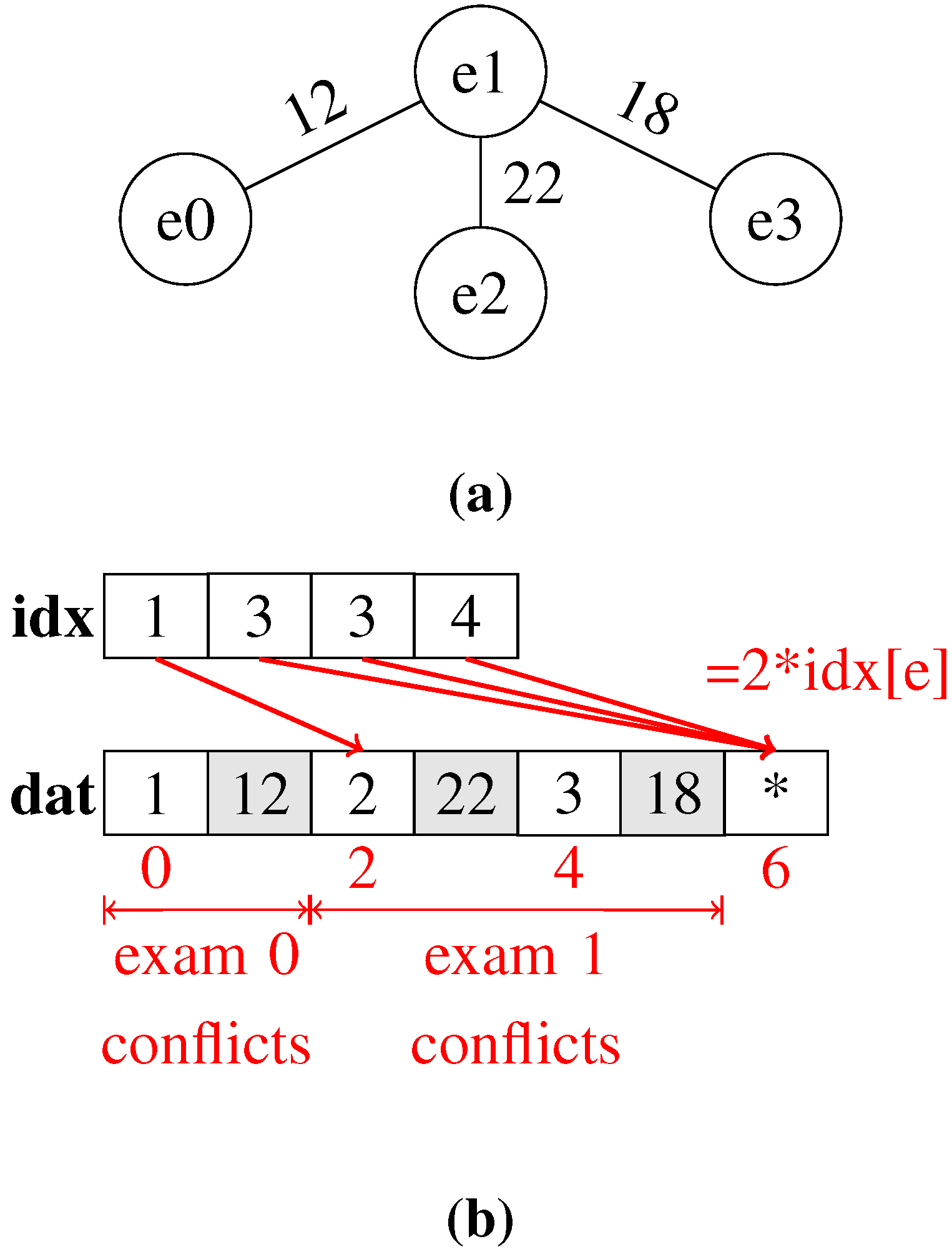
Table 1, the conflict matrix is sparse. Thus, in this work, apart from the full conflict matrix, the compressed sparse row (CSR) format is also used (
Figure 3). In CSR, the sparse matrix becomes a vector of rows,
R. Each row
is a vector of pairs, one for each non-zero element. Each pair contains the non-zero column index and the element value:
In a pre-processing stage, the compressed conflict matrix is calculated in two different forms. One form represents the full conflict matrix, where each examination is associated with each other examination in conflict. The CSR format is equivalent to the adjacency matrix for the conflict graph between the examinations. The other form, more useful for this work, is the diagonal conflict matrix. For every examination
i, the diagonal conflict matrix row
contains only conflicts with examinations indexed with
.
This way, the complexity for the full evaluator is reduced to ), where is the conflict density. The CSR evaluators exploit the sparse features of the conflict matrix.
Figure 3.
(a) Conflict graph for the problem described in the half-compressed conflict matrix figure; (b) half-compressed conflict matrix structure (the dat array contains tuples of the exam in conflict (white) and the conflicting number of students (gray)).
Figure 3.
(a) Conflict graph for the problem described in the half-compressed conflict matrix figure; (b) half-compressed conflict matrix structure (the dat array contains tuples of the exam in conflict (white) and the conflicting number of students (gray)).
5.4. Selection and Reproduction
The next step of the algorithm is the selection of the parents that will form two new children, according to their cost. The tournament selection with a size 3% of the population size and the one-point crossover operator were selected. During the experiments that were done, it was observed that the tournament selection size is of great importance for the performance of the algorithm. For small population sizes, the size of the tournament selection can be small, as well, but as the population size increases, a small tournament selection size does not allow the algorithm to improve the solutions. Thus, the tournament selection size needs to be increased for bigger populations, but this comes with a cost in execution time, and therefore, a balance should be found. After many runs, we ended up in this fraction of the population size.
The two parallelization approaches were implemented for this stage, as well. In the chromosome-threaded approach, each thread selects two chromosomes as parents, according to their costs, and forms two new chromosomes for the next generation. Therefore, only threads are needed. In the examination threaded approach, each thread produces only one gene (time slot of an examination) for each of the two new chromosomes. The problem that arises here is that all of the threads that form a new chromosome should take the same chromosomes as parents and the same cut point. In order to achieve this, the same curandstate was given to each thread, so as to produce the same numbers in its own local variables, thus selecting the same parents and the same cut point. However, the accesses to specific locations of memory from many threads at the same time lead to very bad performance. Therefore, another approach was followed. The selection was separated from the reproduction stage, and they were executed in different kernels, so that each process can have a different number of threads launched. In the selection process, threads are executed and select the parents and the cut point for the threads of the crossover kernel. They store the selected values in arrays in global memory, so that they are later accessible from the threads of the crossover kernel. Then, the reproduction is performed by assigning one thread to each examination. The configuration of threads launched is the same with the examination threaded approach in the evaluation stage, with the only difference being that instead of blocks executed in the y direction, only are launched in this stage. The pseudocodes for the three approaches are given in Algorithms 4–7. The device API of the curand library was used in this stage, as it is not known beforehand the number of random numbers that are needed, as we need to ensure that the chromosomes selected are not the same, and therefore, the curand function may be used a lot of times.
| Algorithm 4: Selection and reproduction, chromosome-threaded approach: each thread produces two new chromosomes. |
![Algorithms 07 00295 i004]() |
| Algorithm 5: Selection and reproduction, examination-threaded approach (one kernel implementation): each thread produces one gene for each of the two new chromosomes. |
![Algorithms 07 00295 i005]() |
| Algorithm 6: Selection, examination-threaded approach (two kernels implementation): each thread selects the parents, the cut point and creates a random number. |
;
;
;
;
;
;
;
;
;
;
|
| Algorithm 7: Reproduction, examination-threaded approach (two kernels implementation): each thread uses the previous selected chromosomes and implements the crossover operation. |
![Algorithms 07 00295 i006]() |
5.5. Mutation
Mutation is used in genetic algorithms to diversify the population. The operator used in this work selects some random examinations according to the mutation rate and changes their time slots also randomly, respecting the time slot limit. As in all previous stages, the two approaches of parallelization were implemented. In the chromosome-threaded approach, each thread is responsible for all of the mutation operations needed in one chromosome. In the examination-threaded approach, another problematic situation had to be resolved. In order for every thread to create a random number, a very big initialization table for the curand_uniform function is needed. Since the size of curandState is 48 bytes, in the big datasets, this could not be implemented, due to a lack of memory space. Therefore, it was decided to use the host API of the curand library in this stage, in order to create the necessary float and integer numbers instead of the curandState array, since they occupy much less memory space. The pseudocode for the two approaches is given in Algorithms 8 and 9.
| Algorithm 8: Mutation, chromosome-threaded approach: each thread mutates the genes in a single chromosome, according to a probability. |
![Algorithms 07 00295 i007]() |
| Algorithm 9: Mutation, examination-threaded approach: each thread mutates a single gene, according to a probability |
![Algorithms 07 00295 i008]() |
5.6. Termination Criterion
Mainly three termination criteria are used in genetic algorithms. The termination of the algorithm after a specific number of generations or after a specific time limit are two of them, while another one is the termination of the algorithm when no progress is achieved for a specific number of generations. In this work, the algorithm terminates after a pre-defined number of generations.
5.7. Greedy Steepest Descent Algorithm
In order to improve the results, in terms of quality, a local search algorithm was implemented that traverses all of the genes of a chromosome one after the other and finds the best time slot that every examination can be scheduled. The process of finding the best time slot for each examination is not independent, because the cost of each examination should be calculated with the time slots of all of the other examinations fixed. Taking into consideration that every block cannot have more than 1024 threads and that the maximum number of available time slots in the datasets is 42, the decision for the configuration of threads was the following:
In the above equations, and are the threads per block in the x- and y-axis, respectively, T is the number of available time slots and is the population size. In this way, the limit of 1024 threads in a block is never overcome. Each thread in a block calculates the cost of an examination with a specific time slot, and then, the time slot with the smaller cost is found. Then, the process is repeated for all of the examinations. The pseudocode is given in Algorithm 10.
| Algorithm 10: Greedy steepest descent algorithm: every thread calculates the cost of an examination for a specific time slot. |
![Algorithms 07 00295 i009]() |
6. Experimental Results
In order to evaluate our algorithm, a number of experiments was designed and executed. In this section, all of the steps of the algorithm are examined in terms of performance. Moreover, the use of the compressed sparse row format instead of the full sparse conflict matrix is analyzed. Two other issues that are discussed are the improvement that the greedy steepest descent algorithm adds to the genetic algorithm and the impact of the tournament selection size as the population grows, in the performance of the algorithm. In the end, the quality results obtained are shown. From the thirteen datasets, in the speedup figures, only four are presented, so that the figures remain easily readable. However, special attention was given in the selection of the datasets to be presented. The datasets chosen are pur-s-93, due to its large size and the special design options that it requires, car-s-91, as the largest from the remaining ones, hec-s-92, as the smallest one, but with the highest conflict density, and lse-f-91, as a medium-size dataset with small conflict density. All of the experiments were conducted in work stations, containing one NVIDIA graphics card GTX580 with 512 cores. The CPUs used had an Intel i7 processor at 3.40 GHz with 16 GB RAM and a solid state disk. It should be mentioned that the serial approach discussed here is single threaded. Given that evolutionary algorithms are stochastic processes, many runs of the algorithm with different parameters were done, and parameters that gave good results were chosen. Only for the speedup section, it should be mentioned that the value of 50% was chosen as a crossover probability in order not to help the GPU achieve better time and, thus, be unfair in the comparison with the CPU, due to divergent execution. Furthermore, it should be added that the selected values are not necessarily the best for all of the datasets, and of course, all of the results depend on the initial seed of the random generator. Parameter values were chosen after a parameter sweep that was performed. Therefore, the crossover probability has been tested for values ranging from a 10% to 95%, mutation probability for values ranging from 0.1% to 2% and tournament selection size assumed values: pop/64, pop/32, pop/16 and pop/8. Runs showed that value pop/32 struck a balance between good results and fast execution times. Regarding the curand library, the default pseudorandom generator, XORWOW, and the default ordering were used.
6.1. Speedups
The main aim of this work was to accelerate the performance of the algorithm, utilizing the GPU as much as possible. In the following, the speedups obtained for all of the stages, evaluation, reproduction, mutation and local search, will be presented. The speedup is calculated by dividing the execution time of the single-threaded serial function, running on the CPU, and the execution time of the parallel function, running on the GPU. The results are the average of 10 runs with a mutation probability of 0.5% and a crossover probability of 50%, and the relative error was up to 4%. In the generation time of the random numbers with the
curand host API, the first time of execution is expensive in terms of time (7 s) [
60], while the next iterations are executed in fractions of a second. Thus, in the speedup calculation of the mutation phase, we did not use the first measurement; however, it was used in the calculation of the whole speedup of the algorithm.
6.1.1. Evaluation
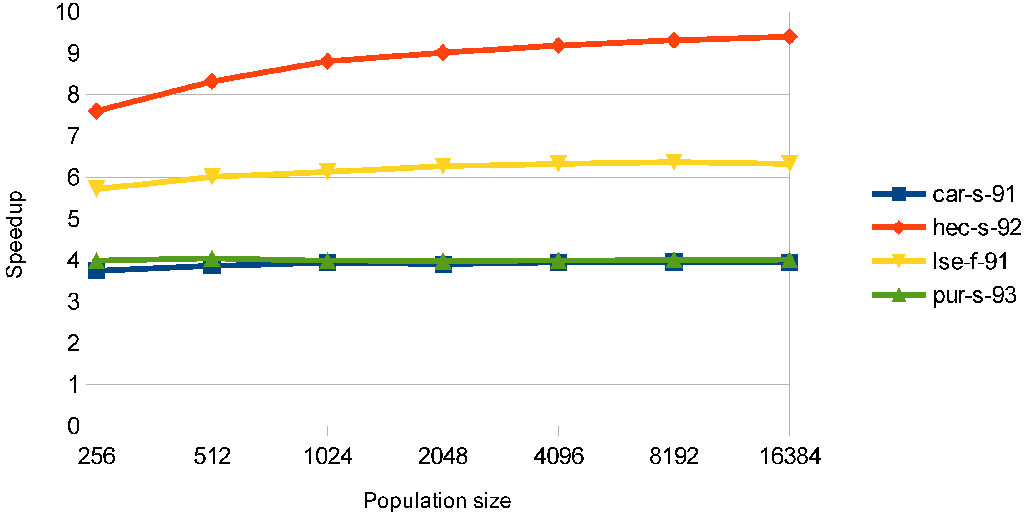
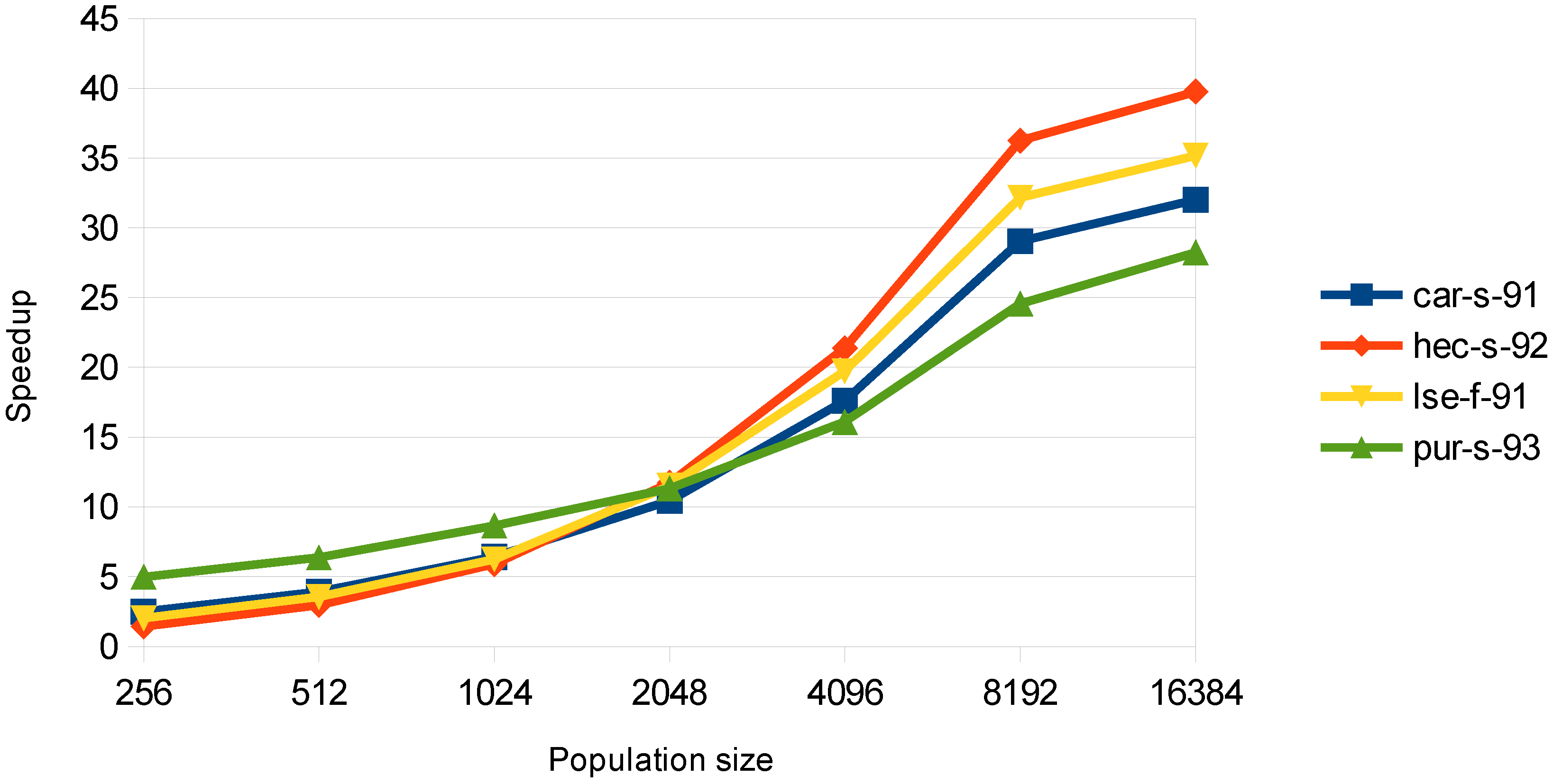
As described in the methodology section, for the evaluation stage, two parallel approaches were implemented. The examination and the chromosome-threaded approach. Moreover, the use of the CSR format was proposed in order to improve the performance, due to the small conflict density of many datasets. In
Figure 4, the speedup obtained with the examination-threaded approach is depicted. This approach gives a better speedup than the chromosome-threaded approach. Moreover, it can be observed that the datasets with the larger speedup are the ones with less courses. This happens, because in the evaluation stage, there is a need for synchronization between the threads and for atomic operations for the big datasets, as explained in the previous section.
Figure 4.
Speedup in the evaluation stage for the examination-threaded approach with the use of the compressed sparse row (CSR) conflict matrix.
Figure 4.
Speedup in the evaluation stage for the examination-threaded approach with the use of the compressed sparse row (CSR) conflict matrix.
6.1.2. Reproduction
In this stage, the examination-threaded approach was faster, as well. In
Figure 5, the speedups achieved for this approach with the implementation with the two different kernels, one for the selection process and one for the reproduction process, are given. We can see here that the speedups increase with the increase in the population size, which means that for low population sizes, the card is not fully utilized. This does not happen in the evaluation stage, and the reason is that the number of blocks of threads in this stage are half of the ones executed in the evaluation stage. Furthermore, the speedups that are achieved in this stage are much greater than in the evaluation stage. This occurs due to the fact that in the reproduction stage, threads access continuous memory locations, leading to memory coalescence, while in the evaluation stage, this is not achieved, synchronization is needed and atomic operations are necessary in big datasets.
Figure 5.
Speedup in the reproduction stage for the examination-threaded approach with the separation of the selection and reproduction stages in different kernels.
Figure 5.
Speedup in the reproduction stage for the examination-threaded approach with the separation of the selection and reproduction stages in different kernels.
6.1.3. Mutation
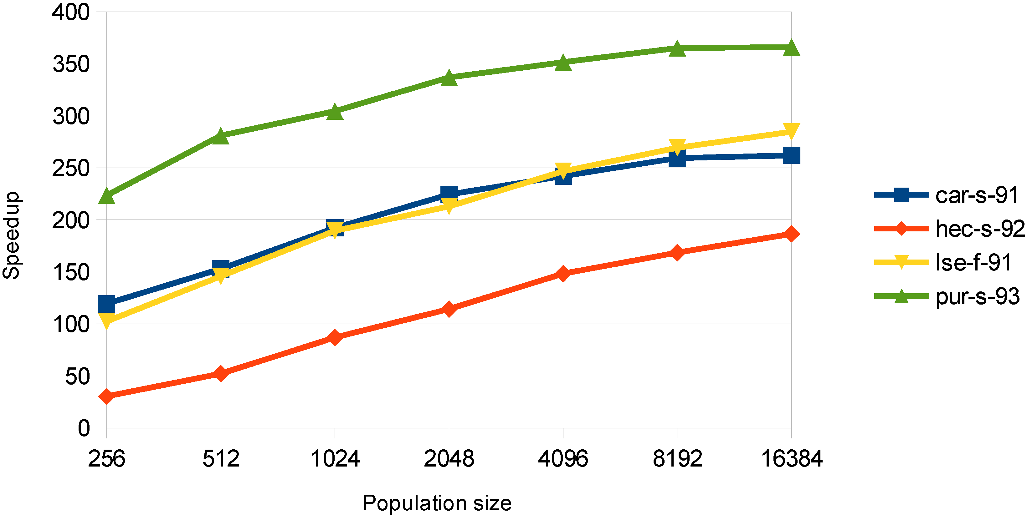
In this stage, both approaches give very large speedup values, but the examination-threaded approach utilizes the card better as it achieves satisfactory speedups from small population sizes. In
Figure 6, the speedup for the examination-threaded approach is illustrated. The speedup for the
pur-s-93 dataset is up to 360×, which is very large, as the mutation phase can be fully parallelized. Although the mutation stage takes only a very small percent of the whole execution time of the algorithm, the achieved speedup values show that this encoding matches well with the GPU architecture.
Figure 6.
Speedup in the mutation stage for the examination-threaded approach.
Figure 6.
Speedup in the mutation stage for the examination-threaded approach.
6.1.4. Greedy Steepest Descent Algorithm
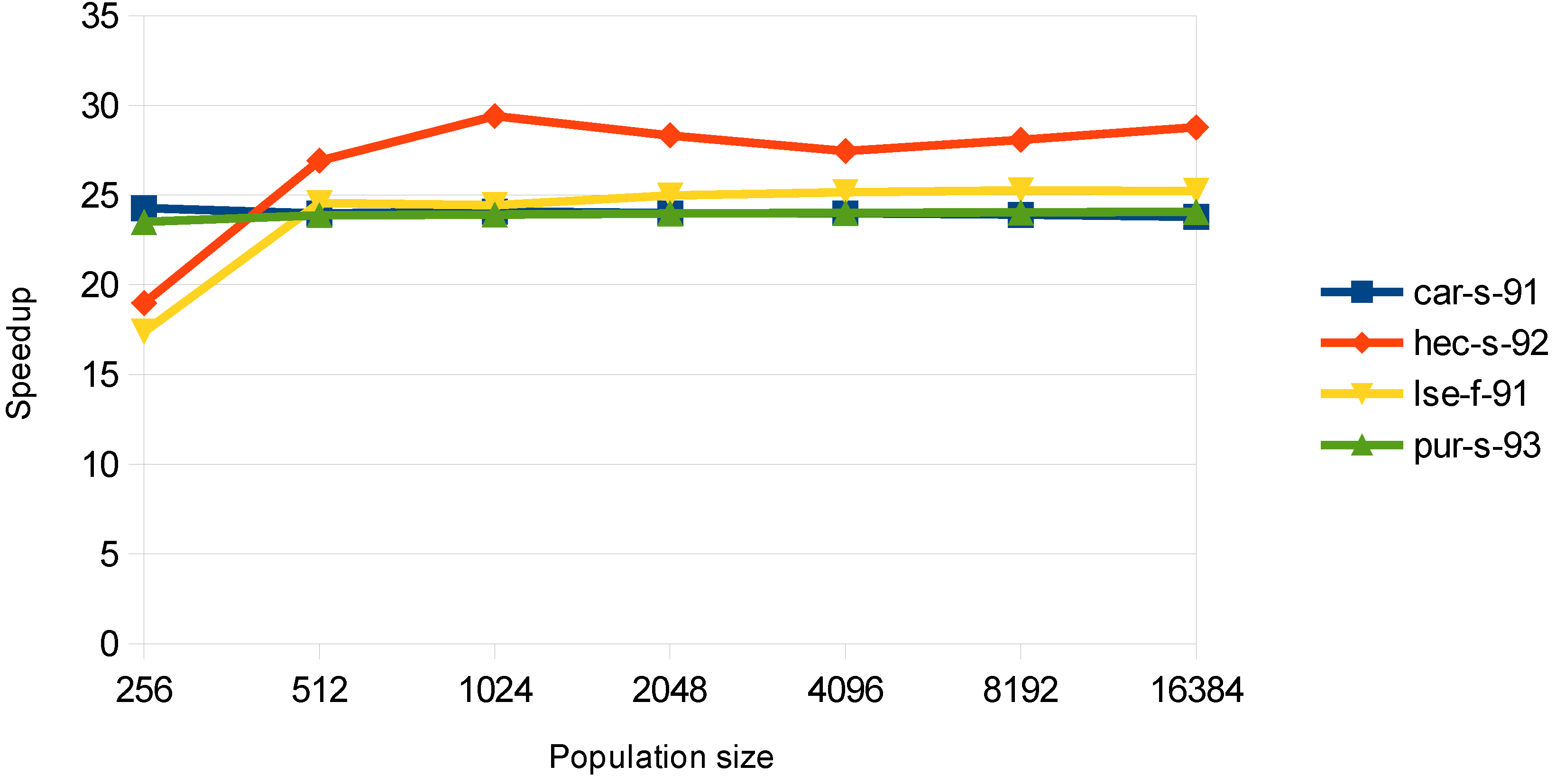
In
Figure 7, the speedup for the steepest descent algorithm is shown. It remains almost constant for all of the population sizes, showing that the card is well utilized. It should also be mentioned that this function is the most time consuming, and thus, the speedup of this process is crucial for the overall performance.
Figure 7.
Speedup in the greedy steepest descent algorithm stage.
Figure 7.
Speedup in the greedy steepest descent algorithm stage.
6.1.5. Total Speedup
The total speedup of the algorithm for the four datasets is shown in
Table 2 for the examination-threaded approach. The transfers of all of the data to and from the GPU are taken into account. The speedup is much larger in population size, 8192, which can be explained by the fact that in small population sizes, the total execution time is dominated by the memory transfers and not the computation and that not a significant number of threads are launched, so that the GPU can be efficient. From
Figure 4,
Figure 5,
Figure 6 and
Figure 7 and from
Table 2, it is shown that the speedup is not increasing much for populations greater than 8192. This can be accredited to the fact that the number of blocks and the number of the total threads increase so much at this point, that the GPU processes them sequentially.
Table 2.
Total speedup for the examination-threaded approach.
Table 2.
Total speedup for the examination-threaded approach.
| Dataset | pop = 256 | pop = 2048 | pop = 8192 | pop = 16,384 |
|---|
| car-s-91 | 4.37 | 4.54 | 21.97 | 23.96 |
| hec-s-92 | 3.26 | 4.73 | 25.372 | 26.17 |
| lse-f-91 | 3.09 | 4.32 | 22.54 | 23.25 |
| pur-s-93 | 4.34 | 4.31 | 22.11 | 21.37 |
6.2. Compressed Sparse Row Format
In
Table 3, the exact execution time on the GPU of the evaluation stage for one generation and population size 256, for the four datasets used and for the implementations, with the full conflict matrix and with the CSR format are presented, along with the achieved speedup and the conflict density. The speedups are the same for all of the population sizes, something expected because the use of the CSR format is only related to the conflict density of the specific dataset. It can be observed that the dataset with the highest conflict density (
hec-s-92) has the smallest speedups, while the dataset with the smallest conflict density (
pur-s-93) has the biggest speedups. The results shown here were obtained from the previous set of measurements.
Table 3.
GPU evaluation execution time and speedup between the full conflict matrix and the compressed sparse row format implementation.
Table 3.
GPU evaluation execution time and speedup between the full conflict matrix and the compressed sparse row format implementation.
| Dataset | Full Conflict Matrix (ms) | CSR Conflict Matrix (ms) | Speedup | Conflict Density |
|---|
| car-s-91 | 20.80 | 3.97 | 5.24 | 0.13 |
| hec-s-92 | 0.12 | 0.09 | 1.29 | 0.42 |
| lse-f-91 | 5.52 | 0.41 | 13.44 | 0.06 |
| pur-s-93 | 377.09 | 11.50 | 32.78 | 0.03 |
6.3. Improvement with the Greedy Steepest Descent Algorithm
In this subsection, the improvement of the quality of the solutions that occurs with the additional step of the greedy steepest descent algorithm, is examined. In
Table 4, the average distance (%) from the best reported solutions in the literature, for all of the datasets with the genetic algorithm, is illustrated. In
Table 5, the respective values for the hybrid evolutionary algorithm are given. The results are from five runs for three population sizes with different seeds and a small number of initial solutions. The only dataset with no initial solutions was
pur-s-93. The mutation probability was 0.8% and the crossover probability 30%. The distance from the best solution with the steepest descent algorithm is smaller for all of the datasets. In the next Tables when the algorithm failed to provide a feasible solution with the selected parameters it is denoted using INF which stands for infeasible.
Table 4.
Average distance (%) from the best reported solution in the bibliography with the genetic algorithm.
Table 4.
Average distance (%) from the best reported solution in the bibliography with the genetic algorithm.
| Dataset | pop = 256 | pop = 2048 | pop = 16,384 |
|---|
| car-f-92 | 89.68 | 89.41 | 58.46 |
| car-s-91 | 110.67 | 110.67 | 80.40 |
| ear-f-83 | 74.85 | 64.78 | 56.94 |
| hec-s-92 | 91.06 | 80.73 | 74.10 |
| kfu-s-93 | 91.80 | 58.66 | 38.87 |
| lse-f-91 | 113.42 | 70.32 | 59.98 |
| pur-s-93 | INF | INF | INF |
| rye-s-93 | 153.7 | 149.91 | 94.54 |
| sta-f-83 | 19.43 | 19.43 | 19.23 |
| tre-s-92 | 57.04 | 48.06 | 42.17 |
| uta-s-92 | 81.56 | 81.56 | 65.40 |
| ute-s-92 | 35.83 | 25.88 | 19.85 |
| yor-f-83 | 41.41 | 37.12 | 30.41 |
Table 5.
Average distance (%) from the best reported solution in the bibliography with the hybrid evolutionary algorithm.
Table 5.
Average distance (%) from the best reported solution in the bibliography with the hybrid evolutionary algorithm.
| Dataset | pop = 256 | pop = 2048 | pop = 16,384 |
|---|
| car-f-92 | 42.21 | 29.40 | 26.77 |
| car-s-91 | 44.84 | 30.27 | 24.95 |
| ear-f-83 | 43.16 | 33.77 | 28.88 |
| hec-s-92 | 30.87 | 27.02 | 20.78 |
| kfu-s-93 | 24.17 | 16.15 | 12.53 |
| lse-f-91 | 43.20 | 29.03 | 27.43 |
| pur-s-93 | 263.7 | 153.23 | 126.06 |
| rye-s-93 | 54.01 | 36.38 | 33.36 |
| sta-f-83 | 16.83 | 16.69 | 16.64 |
| tre-s-92 | 22.88 | 19.42 | 13.85 |
| uta-s-92 | 43.95 | 30.13 | 25.57 |
| ute-s-92 | 7.52 | 5.43 | 4.53 |
| yor-f-83 | 17.64 | 13.40 | 11.31 |
6.4. Tournament Selection Size
Another interesting point that occurred during the development of the algorithm is the size of the tournament selection of the genetic algorithm as the population size increases. It is obvious that as the population size increases, a small tournament selection size results in small improvement of the quality of the solutions. Thus, it was decided to increase the tournament selection size as the population size increases. For this reason, we chose the tournament selection size to be a fraction of the population size. However, the bigger the size of the tournament selection, the more computational time that is required. A balance was obtained for
. In
Table 6 and
Table 7, the average distance from the best reported solution in the literature for a constant tournament selection size (10) and for a fraction of population size (
) is illustrated. The experiments were run five times for all thirteen datasets for three population sizes, with different seeds, but the same initial solutions, and the mutation probability was 0.3% and the crossover probability 75%. Furthermore, the steepest descent algorithm was excluded from these measurements, so that it could not impact the quality of the solutions. It is clearly seen that with a larger tournament selection size, the algorithm obtains better solutions in population sizes of 2048 and 16,384. For a population size of 256, the tournament selection size (10) is greater than the fraction of the population size (256/32 = 8). It is worth mentioning that in general, it is here illustrated that bigger population sizes give better solutions.
Table 6.
Average difference (%) from the best reported solution in the bibliography with the genetic algorithm and a tournament selection size of 10.
Table 6.
Average difference (%) from the best reported solution in the bibliography with the genetic algorithm and a tournament selection size of 10.
| Dataset | pop = 256 | pop = 2048 | pop = 16,384 |
|---|
| car-f-92 | 77.73 | 66.69 | 63.97 |
| car-s-91 | 90.09 | 82.24 | 78.27 |
| ear-f-83 | 67.90 | 58.75 | 61.48 |
| hec-s-92 | 66.13 | 59.39 | 58.09 |
| kfu-s-93 | 52.36 | 46.04 | 45.46 |
| lse-f-91 | 67.17 | 64.63 | 63.47 |
| pur-s-93 | INF | INF | INF |
| rye-s-93 | 119.01 | 106.42 | 94.77 |
| sta-f-83 | 19.43 | 19.43 | 19.42 |
| tre-s-92 | 53.26 | 49.31 | 41.63 |
| uta-s-92 | 80.02 | 73.28 | 71.11 |
| ute-s-92 | 30.02 | 33.75 | 31.53 |
| yor-f-83 | 37.82 | 35.69 | 34.25 |
Table 7.
Average difference (%) from the best reported solution in the bibliography with the genetic algorithm and a tournament selection size of .
Table 7.
Average difference (%) from the best reported solution in the bibliography with the genetic algorithm and a tournament selection size of .
| Dataset | pop = 256 | pop = 2048 | pop = 16,384 |
|---|
| car-f-92 | 81.40 | 61.34 | 46.17 |
| car-s-91 | 94.92 | 60.79 | 50.19 |
| ear-f-83 | 65.67 | 56.00 | 49.19 |
| hec-s-92 | 71.63 | 54.45 | 54.68 |
| kfu-s-93 | 57.49 | 41.70 | 38.46 |
| lse-f-91 | 77.11 | 53.93 | 50.95 |
| pur-s-93 | INF | INF | INF |
| rye-s-93 | 123.55 | 81.60 | 83.19 |
| sta-f-83 | 19.43 | 19.43 | 18.84 |
| tre-s-92 | 48.74 | 39.40 | 35.03 |
| uta-s-92 | 80.55 | 61.57 | 48.31 |
| ute-s-92 | 31.05 | 25.25 | 17.71 |
| yor-f-83 | 38.58 | 32.22 | 27.03 |
6.5. Quality of Solutions
Regarding the quality of the solutions achieved, in this section, a statistical analysis based on the results is given. Given that in this work, the computational power of a GPU is utilized, large population sizes are used. In
Table 8, the minimum, the maximum and the average costs of the solutions achieved for all of the datasets and a population size of 256 are given. In
Table 9, the same metrics are given for a population size of 16,384. Furthermore,
Figure 8 and
Figure 9 show descriptive statistics for the measurements. There was a need for normalization, since the costs were not of the same magnitude. Thus, the average cost has taken the value of 100 for all of the datasets, and the remaining statistics were calculated. For the
sta-f-83 dataset in
Figure 8 and
Figure 9, there is no box, as the initial and the best solution are very close and with a high cost (157–160). The measurements were done with identical seeds (1–100) to the
function of the C programming language. The mutation probability was 0.6%, the crossover probability 50% and the number of generations 200 for all of the experiments. It can be seen that all of the results gained for the bigger population size are better. This is something expected, since by having a larger population size, a bigger part of the solution space is explored.
Table 8.
Minimum, maximum and average cost with a population size of 256.
Table 8.
Minimum, maximum and average cost with a population size of 256.
| Dataset | Minimum Cost | Maximum Cost | Average Cost |
|---|
| car-f-92 I | 4.86 | 5.32 | 5.04 |
| car-s-91 I | 5.72 | 6.33 | 5.92 |
| ear-f-83 I | 39.05 | 42.52 | 40.24 |
| hec-s-92 I | 11.34 | 12.91 | 12.27 |
| kfu-s-93 I | 15.45 | 16.98 | 16.14 |
| lse-f-91 I | 12.06 | 13.37 | 12.68 |
| pur-s-93 I | 10.75 | 33.64 | 21.51 |
| rye-s-93 I | 9.20 | 10.48 | 9.63 |
| sta-f-83 I | 157.38 | 157.70 | 157.47 |
| tre-s-92 I | 9.15 | 9.75 | 9.51 |
| uta-s-92 I | 4.05 | 4.33 | 4.20 |
| ute-s-92 I | 25.43 | 27.18 | 26.19 |
| yor-f-83 I | 39.52 | 42.41 | 41.32 |
Table 9.
Minimum, maximum and average cost with a population size of 16,384.
Table 9.
Minimum, maximum and average cost with a population size of 16,384.
| Dataset | Minimum Cost | Maximum Cost | Average Cost |
|---|
| car-f-92 I | 4.77 | 5.06 | 4.92 |
| car-s-91 I | 5.32 | 5.84 | 5.60 |
| ear-f-83 I | 37.27 | 39.82 | 38.65 |
| hec-s-92 I | 10.88 | 12.14 | 11.39 |
| kfu-s-93 I | 14.48 | 16.00 | 15.33 |
| lse-f-91 I | 11.22 | 12.62 | 11.93 |
| pur-s-93 I | 5.25 | 14.99 | 8.36 |
| rye-s-93 I | 8.64 | 9.32 | 8.98 |
| sta-f-83 I | 157.20 | 157.45 | 157.39 |
| tre-s-92 I | 8.72 | 9.61 | 9.17 |
| uta-s-92 I | 3.64 | 4.13 | 3.90 |
| ute-s-92 I | 25.11 | 26.71 | 25.58 |
| yor-f-83 I | 38.80 | 41.21 | 40.05 |
Figure 8.
Descriptive statistics chart for population size 256.
Figure 8.
Descriptive statistics chart for population size 256.
Figure 9.
Descriptive statistics chart for a population size of 16,384.
Figure 9.
Descriptive statistics chart for a population size of 16,384.
The approach of this paper achieved competitive results for many of the Carter/Toronto datasets. In
Table 10, the best costs from this work, from other evolutionary techniques and the best available in the literature are shown. IGA stands for Informed Genetic Algorithm, MMAS for Max Min Ant System and hMOEA for hybrid Multi-Objective Evolutionary Algorithm. In bold characters are the best values among the evolutionary approaches. The table shows that in four datasets, this work achieves a better cost than alternative evolutionary approaches. Another conclusion drawn from this table is that evolutionary approaches do not manage to get the best cost in any of the datasets of this problem.
Table 10.
A comparison with other evolutionary approaches and the best solution reported.
Table 10.
A comparison with other evolutionary approaches and the best solution reported.
| Dataset | This Work | IGA [38] | hMOEA [35] | MMAS [34] | Ersoy [39] | Best |
|---|
| car-f-92 | 4.47 | 4.2 | 4.2 | 4.8 | - | 3.74 [61] |
| car-s-91 | 5.24 | 4.9 | 5.4 | 5.7 | - | 4.42 [61] |
| ear-f-83 | 34.41 | 35.9 | 34.2 | 36.8 | - | 29.3 [30] |
| hec-s-92 | 10.39 | 11.5 | 10.4 | 11.3 | 11.6 | 9.2 [30] |
| kfu-s-93 | 13.77 | 14.4 | 14.3 | 15.0 | 15.8 | 12.81 [62] |
| lse-f-91 | 11.06 | 10.9 | 11.3 | 12.1 | 13.2 | 9.6 [30] |
| pur-s-93 | 5.25 | 4.7 | - | 5.4 | - | 3.7 [30] |
| rye-s-93 | 8.61 | 9.3 | 8.8 | 10.2 | - | 6.8 [30] |
| sta-f-83 | 157.05 | 157.8 | 157.0 | 157.2 | 157.7 | 134.70 [28] |
| tre-s-92 | 8.51 | 8.4 | 8.6 | 8.8 | - | 7.72 [62] |
| uta-s-92 | 3.63 | 3.4 | 3.5 | 3.8 | - | 3.06 [61] |
| ute-s-92 | 24.87 | 27.2 | 25.3 | 27.7 | 26.3 | 24.21 [63] |
| yor-f-83 | 37.15 | 39.3 | 36.4 | 39.6 | 40.7 | 34.78 [62] |
| normalized | 16.51% | 17.14% | 21.11% | 25.23% | - | - |
| |
6.6. Limitations and Advantages
The main limitation in this problem was that most datasets were too large to fit in the small shared memory of the multiprocessors of the GPU. However, this approach could be beneficial for other timetabling problems, as well. Despite the fact that many papers exist for the acceleration of genetic algorithms with the use of GPUs, to our knowledge, there is no work dealing with this kind of problem and the use of GPUs. Moreover, it should be mentioned that the speedup gained from a GPU is dependent on the computations that need to be performed. Given that the objective function of our problem is not too complicated, greater speedups can be expected in problems with more complex objective functions.

 ,
, 


