1. Introduction and Related Work
Approximate string matching (ASM) is an important problem that arises in applications related to text searching, pattern recognition, signal processing, and computational biology, to name a few. The problem consists in locating all the occurrences O of a given pattern string P, of size m, in a larger text string T, of size u, where the distance between P and O is less than a given threshold k. We focus on the edit distance, that is, the minimum number of character insertions, deletions, and substitutions of single characters to convert one string into the other.
The classical sequential search solution runs in
worst-case time (see [
1]). An optimal average-case algorithm requires
time [
2,
3], where
σ is the size of the alphabet Σ. Those good average-case algorithms are called
filtration algorithms: they traverse the text fast while checking for a simple necessary condition, and only when this condition holds do they verify the text area using a classical ASM algorithm. For long texts, however, sequential searching might be impractical as it must scan all the text. To avoid the scanning we use an
index [
4,
5], which is a data structure built on the text.
There exist indexes specifically devoted to ASM [
6,
7,
8,
9] (see [
5] for an overview). Most are oriented to worst-case performance, and experiment a space-time barrier: They require either exponential time (in
m or
k), or exponential index space (
e.g., integers). This renders them impractical in many applications. Another choice is to reuse an index designed for exact searching, all of which are linear-space (
i.e. integers), and try to do ASM over it. Indexes such as suffix trees [
10], suffix arrays [
11], or based on so-called
q-grams or
q-samples [
4], have been used for ASM. There exist several algorithms, based on suffix trees or arrays, which focus on worst-case performance [
12,
13,
14]. They suffer from the same space-time barrier, achieving a search time independent of
u but exponential in
m or
k. Essentially, they backtrack on the suffix tree or array, simulating the sequential search over all the text suffixes, and take advantage of the factoring of similar substrings achieved by suffix trees or arrays.
Indexes based on
q-grams or
q-samples are appealing because they require less space than suffix trees or arrays. The algorithms on those indexes do not offer worst-case guarantees, but perform well on average when the
error level is low enough, say
. Those indexes basically simulate a sequential filtration algorithm, such that the “necessary condition” checked involves exact matching of pattern substrings, and as such can be verified with any exact-searching index. Such filtration indexes,
e.g., [
15,
16], cease to be useful for moderate
α levels that are still of interest in applications.
The most successful approach, in practice, is in between backtracking and exact-matching filtration, and is called
hybrid indexing. The index determines the text positions to verify using an approximate-matching condition over pattern pieces. Those positions are determined using backtracking, whose time is exponential in the length of the string or the number of errors. Yet, it is applied over short pattern pieces and allowing few errors, so that the exponential cost is controlled. Indexes of this kind offer average-case guarantees of the form
for some
, and work well for higher error levels. They have been implemented over
q-gram indexes [
17], suffix arrays [
18], and
q-sample indexes [
19].
Yet, many of those linear-space indexes are very large anyway. For example, suffix arrays require 4 times the text size and suffix trees require at the very least 10 times [
20]. In recent years a new and extremely successful class of indexes has emerged.
Compressed full-text indexes use data compression techniques to produce less space-demanding data structures [
21]. It turns out that data compression algorithms exploit the internal structure of a string much in the same way indexes do, and therefore it is possible to build a compressed index that takes space proportional to that of the compressed text, offers indexed searching, and replaces the text as it can reproduce any text substring (in which case they are called
self-indexes). The size of those indexes is measured in terms of the empirical text entropy,
[
22], which gives a lower bound on the number of bits per symbol achievable by a
k-th order compressor. There are two main families of self-indexes [
21]. One is based on Ziv-Lempel compression [
23,
24,
25,
26,
27,
28], and the other simulates suffix trees and suffix arrays [
24,
29,
30,
31,
32,
33,
34,
35].
Compressed indexes usually require more operations than their classical counterpart, yet they can operate on a smaller/faster memory in the hierarchy. This is particularly noticeable when they can fit in RAM while the classical indexes must operate on disk. In this case their advantages are most striking. A recent survey covers the practical state of the art in compressed self-indexes [
36].
Despite their great success, self-indexes have been mainly used for exact searching. Only very recently some indexes taking
or
bits have appeared [
8,
37,
38]. Those are specifically designed for ASM, focus on worst case, and unfortunately require time exponential in
k [
5].
Instead, in this paper we are interested in carrying out ASM over existing compressed full-text self-indexes, and in achieving good practical performance. We start by implementing the exact-match filtration approach over compressed self-indexes. This is the most direct solution because these indexes already provide exact searching. We choose a Ziv-Lempel self-index [
25], as this type of index is fast to extract the text areas to be verified, and we optimize the process of extracting those text passages. We also try a suffix-array self-index [
24] as these permit efficiently counting the number of occurrences, which allows us to optimize the pattern partitioning.
Then we turn our attention to hybrid indexing, which has been very successful on classical indexes. We show how the ideas of hybrid indexing over
q-sample indexes [
19] can be carried over Ziv-Lempel indexes, by regarding the text parsing as an irregular variant of the
q-sampling. We obtain novel results about
q-sample indexes that may find applications beyond compressed indexes.
Finally, we focus on suffix-tree-based self-indexes. Any ASM algorithm over suffix trees can be adapted to work over compressed ones. However, some adjustments are necessary because accessing the text in a self-index is around two orders of magnitude slower than in plain form. To address this problem we study the hierarchical verification technique [
17,
39] and show that it can benefit from
bidirectionality, that is, by extending edit distance computation from both ends of the string. This is particularly relevant on this type of self-indexes, as they permit moving in the text in either direction. This second index is slower than the Lempel-Ziv-based one, but it takes significantly less space. Both hybrid indexing techniques improve upon the results obtained with the exact-matching approach.
The paper has the following structure. In
Section 2. we review some basic concepts about ASM, define some notation, and describe our contributions.
Section 3. describes our application of exact-matching filters for ASM over self-indexes.
Section 4. and
Section 5. are dedicated to hybrid ASM over Lempel-Ziv compressed indexes. In
Section 4. we explain our approach over a general
q-samples index, but we assume the size of the samples is fixed. In
Section 5. we tackle the problem of an irregular parsing.
Section 6. is dedicated to our second hybrid approach,
i.e. ASM over compressed suffix trees.
Section 7. gives experimental results comparing all of our approaches with each other and with other ASM compressed indexes. The paper finishes with
Section 8., where we draw some conclusions and point out future research directions.
Preliminary versions of our results were presented in
SPIRE [
40,
41]. In this paper we include previously unpublished ASM algorithms based on exact partitioning (
Section 3.), as well as more exhaustive material on the previously published algorithms: the proofs of all the lemmas, illustrative examples of the algorithms, a characterization of homogeneous LZ-phrases (
Section 5.3.), and more exaustive experimental results (
Section 7.).
2. Basics and Contribution Overview
2.1. Basic Concepts
We denote by T the text string, by P the pattern string, and by O an occurrence of P in T; by Σ the strings’ alphabet, of size σ; by the symbol (or character) at position of T; by the concatenation of strings; by respectively a prefix, a substring, and a suffix of a string S; by that S is a substring of ; and by ε the empty string.
A
trie is a character-labeled tree where no two children of a node have the same label. The concatenation of the labels from the root to a node
v is called the
path-label of
v, and also denoted
v. A
compact trie is obtained by collapsing the unary paths in a trie into single edges, labeled with the concatenation of the collapsed symbols. The
suffix tree [
10,
42] of
T is a compact trie such that each suffix of
is the path-label of a leaf and vice versa, where
is a terminator symbol. String labels in a suffix tree are substrings of
T, thus they can be represented by a starting position in
T plus a length. We will assume that
u is the length of
. The
suffix array [
11]
stores the suffix indexes of the leaves in lexicographical order. The suffix tree nodes can be identified with suffix array intervals: each node
v corresponds to the range of leaves that descend from
v. For a detailed explanation see,
e.g., Gusfield’s book [
43].
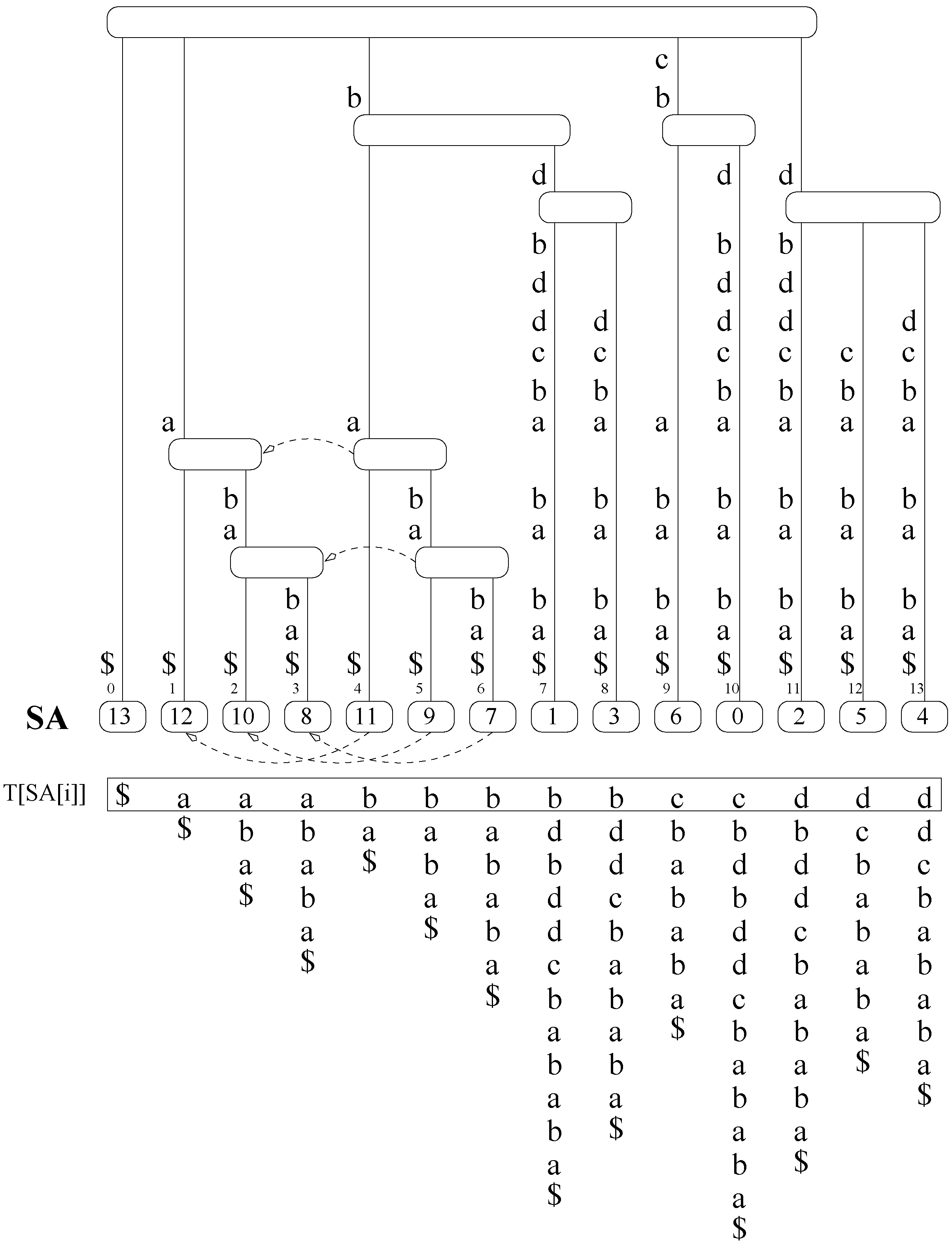
Figure 1 shows an example of a suffix tree and a suffix array.
Ziv-Lempel compression [
23,
44,
45,
46] is based on cutting a text
T into
phrases of varying length, so that, essentially, each phrase already appears somewhere earlier in the text. Each phrase is encoded usually with a fixed number of bits, so more compressible texts generate longer phrases. There are many variants of this family, which basically differ in the rules to form the phrases from the previous text.
2.2. Approximate String Matching
The edit or Levenshtein distance between two strings, , is the smallest number of edit operations that transform A into B. Valid operations are insertions, deletions, and substitutions of characters. Assuming we have a text T, the problem we are interested in solving in this paper is: Given a pattern P and an error limit k, determine all the (starting or ending positions of) substrings O of T for which . We now review the most basic techniques related to this problem. As our running example consider that , and . The only occurrence O in T is .
Figure 1.
On top, suffix tree for . Some suffix links are shown (dashed arrows). On the bottom, suffix array of T.
Figure 1.
On top, suffix tree for . Some suffix links are shown (dashed arrows). On the bottom, suffix array of T.
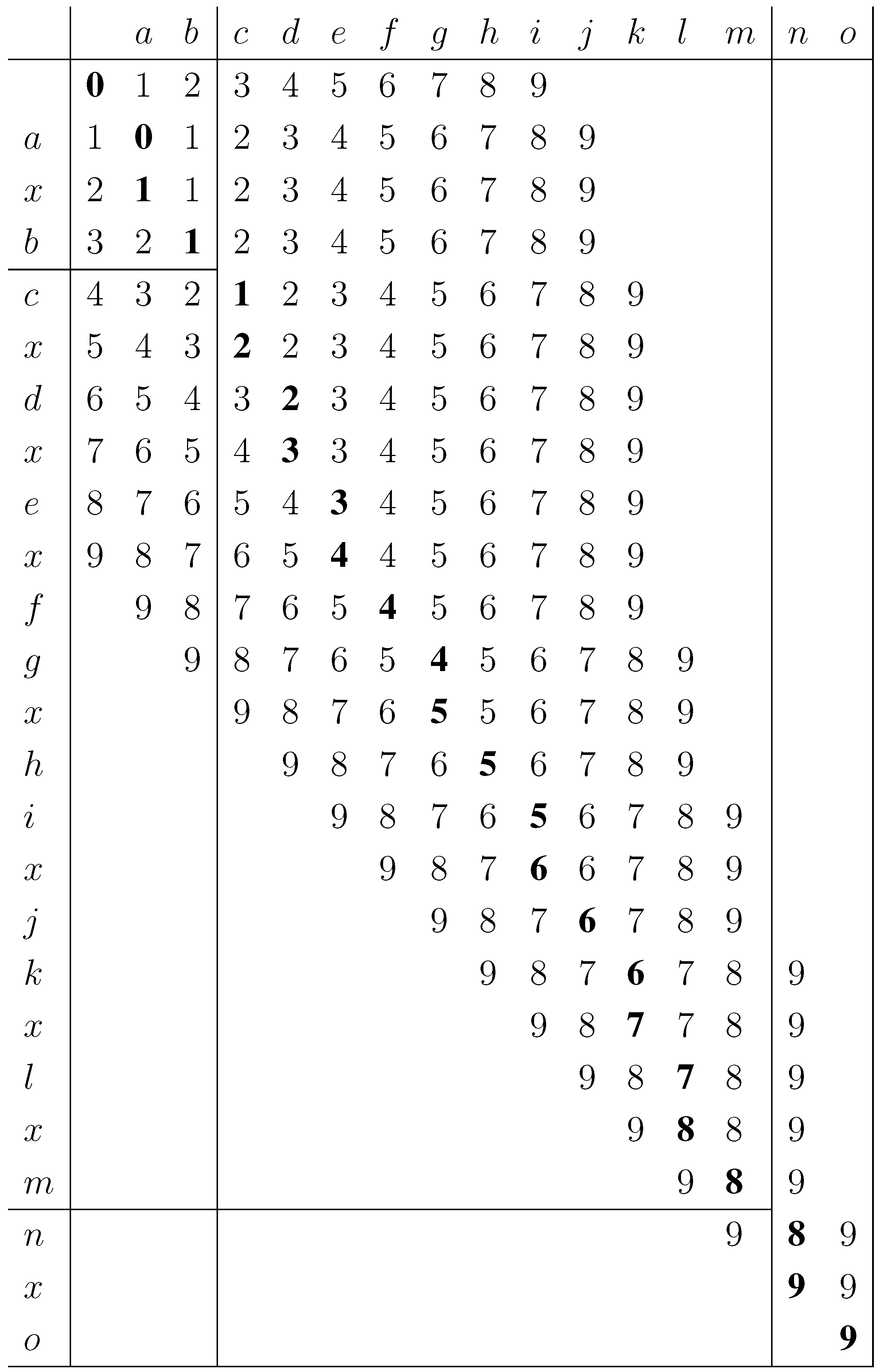
Dynamic programming. There is a well-known dynamic programming (DP) algorithm that computes matrix
D, where
is the edit distance between the prefixes
and
of
A and
B.
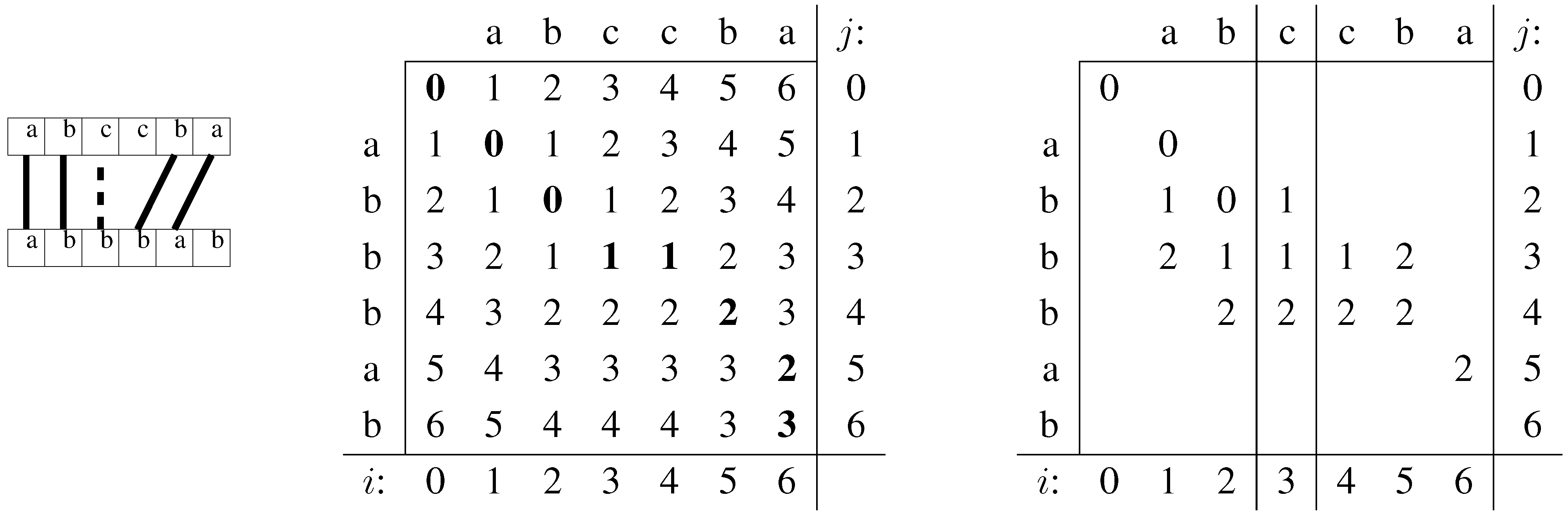
Figure 2 (middle) shows an example of matrix
D for
and
. By looking at cell
we can conclude that
. Let the size of
A and
B be
m and
respectively. This matrix can be computed, in
time, by setting
and
is 0 if
and 1 otherwise. Ukkonen [
47] noted that in order to find cells in
D whose value is
k there is no need to compute cells with a value larger than
k; those can be replaced by
. The remaining cells are referred to as
active cells. With this method, extending the computation of
to
or
requires only
time: All we need to compute is another row, which can contain at most
entries that are
(as
).
Figure 2.
D table computation for strings and . Left: schematic representation of the alignment. Middle: computation of D. The numbers in bold correspond to the alignment shown on the left, and to the shortest path. Right: computation with increasing error bound.
Figure 2.
D table computation for strings and . Left: schematic representation of the alignment. Middle: computation of D. The numbers in bold correspond to the alignment shown on the left, and to the shortest path. Right: computation with increasing error bound.
One can regard the edit distance matrix as an edit graph: Each matrix position is a node, which is the source of three arrows towards (of weight 1), (of weight 1), and (of weight ). Hence is the weight of the shortest path from to .
Backtracking. A way of performing ASM over indexed text is as follows. Perform a depth-first search over the suffix tree of
T, processing one letter at a time, while simultaneously computing the
D table for
P and
, where
is the path-label of the node we are visiting. This table can be used to control the search. When we reach a point
such that
,
i.e. ,
is reported as an occurrence. Usually we also report all the positions in
T at which
occurs, which means traversing the whole sub-tree of
and reporting all its leaf positions. Otherwise if
but there is at least one active cell in the last row,
i.e. for some
i, this means that
and therefore
can potentially be extended into an occurrence, thus the search is allowed to proceed. If, on the other hand, there are no active cells in the last row of
D, the search within the subtree of the current node can be abandoned. For example, by looking at
Figure 2 we can conclude that the search should not proceed further after
because there are no active cells in the last row of the table. Also, since all the other rows contain active cells, this point is indeed reached by the search. It helps to think of
D as a stack of rows that is growing downwards. Note that it is a convenient coincidence that the difference between the
D tables of
and
is only the last row. This means that we can move between these two tables simply by adding or removing a row. At each step the DFS algorithm either pushes a new element into the stack,
i.e. moves from
to
, or it removes a row from the stack,
i.e. moves from
to
. The problem with backtracking is that the number of nodes it visits is at least exponential in
k, and usually in
m. Nevertheless, this process will be a key ingredient in our algorithms.
Filtration and sampling. Filtration algorithms build on the following lemma, simplified from [
4].
Lemma 1 Let A and B be strings such that . Let , for any . Then there is a substring of B and an i such that .
Consider for example and , , , and . Since and , we can conclude that there is a substring of B and an i such that . In particular . In this case we also have that .
Note from the example that, if
, then the
’s can be matched within
B with zero errors, that is, using exact matching. If we assume that
and
B is contained in
O, we can partition
P into
j non-overlapping parts and search
T for them. Thus we must be able to find any text substring with the index (exactly [
16] or approximately [
17,
18], depending on
j). Thus we must use a suffix tree or array [
18], or even a
q-gram index if we never use pieces of
P longer than
q [
16,
17] (a
q-gram index collects all text substrings of length
q and stores a list of the positions of each different such text substring). The contexts around the occurrences found are then examined (say, with dynamic programming) for full occurrences of
P.
Alternatively, if we assume that
and
A is contained in
O, then we can index each
s-th text
q-gram (for some
), to form a so-called
q-samples index. The different text
q-samples are stored into, say, a trie data structure. This trie is traversed to find
q-samples that match within
P with at most
errors. The contexts around those
q-samples are then verified. This works as long as
q and
k are sufficiently small compared to
m. More precisely, any occurrence
O of
P is of length at least
. Wherever an occurrence lies, it must contain at least
complete
q-samples, and this defines
s. This the basis of an “approximate
q-samples” index [
19].
2.3. Our Contributions
Reducing to exact matching of pattern pieces. One can use
any compressed self-index to implement a filtration ASM method that relies on looking for exact occurrences of pattern substrings, as this is what all self-indexes provide. This is our approach in
Section 3.. We first use a Lempel-Ziv index [
25]. The Lempel-Ziv index works well because it is faster to extract the text to verify (recall that in self-indexes the text is not directly available). The specific structure of the Lempel-Ziv index used allows several interesting optimizations, such as factoring out the work of several text extractions. This is possible only when the occurrences span a single Ziv-Lempel phrase. We also use a compressed suffix array [
24], as it permits fast counting of the number of occurrences of any substring. This allows us to quickly find the best partition
so that the number of text verifications is minimized.
Hybrid indexing on Ziv-Lempel indexes. In
Section 4. and
Section 5. we turn our attention to hybrid indexing, which is more complex but promises handling higher error levels
α more efficiently. We still stick to a Ziv-Lempel index, as it allows fast extracting of text contexts. Considering the complications of Ziv-Lempel indexes when occurrences span more than one phrase, we pay special attention to this problem. A good choice to handle this turns out to be another Ziv-Lempel index [
28], whose suffix-tree-like structure is useful for this approximate searching.
Mimicking
q-sample indexes is particularly useful for our goals. A Lempel-Ziv parsing can be regarded as an irregular sampling of the text, and therefore our goal, in principle, is to adapt the techniques of the approximate
q-samples index [
19] to an irregular parsing (thus we must stick to the interpretation
, recall
Section 2.2.). As desired, we would not need to consider occurrences spanning more than one phrase. Moreover, the trie of phrases stored by all Lempel-Ziv self-indexes is the exact analogous of the trie of
q-samples. Thus we can search without requiring further structures.
The irregular parsing poses several challenges. There is no way to ensure that there will be a minimum number j of phrases contained in an occurrence. Occurrences could even be fully contained in a phrase!
We develop several tools to face those challenges. (1) We give a new variant of Lemma 1 that distributes the errors in a convenient way when the samples are of varying length. (2) We introduce a new filtration technique where the samples that overlap the occurrence (not only those contained in the occurrence) can be considered. This is of interest even for classical q-sample indexes. (3) We search for q-samples within long phrases to detect occurrences even if they are within a phrase. This technique also includes novel insights.
Hybrid indexing on compressed suffix trees. Finally, in
Section 6. we explore the impact of
hierarchical verification on hybrid searching, using a compressed suffix tree instead of a Lempel-Ziv index. Hierarchical verification means that an area that needs to be verified is not immediately checked with the maximum number of errors; instead the error threshold is raised gradually. This technique was originally proposed for a hybrid index [
17] and later extended and used for a sequential algorithm [
39]. However, these approaches used hierarchical verification directly over the text
T, meaning that none of the repeated computation was factorized. We investigate precisely how to do this computation over the index, thus allowing us to avoid repeated computation. A key ingredient to achieve our goal is
bidirectionality, that is, the ability of extending the distance computation to the left or to the right of the matched part.
Algorithms for computing edit distance are typically unidirectional, computing from left to right, because they are based on dynamic programming or automata. Interestingly this computation was made bidirectional more than 10 years ago [
48]. They showed how to obtain the edit distance for strings
A and
by extending that for for strings
A and
B, where
c is a letter.
Fortunately enough, most compressed suffix trees and arrays support bidirectionality. Typical indexes, classical suffix trees in particular, are unidirectional, meaning that they can search only by adding letters at the end of the search pattern. Due to the
Rank/
Select duality [
21], bidirectionality arises naturally in a wide class of compressed indexes (Although not usual, there are some non-compressed indexes, such as affix trees [
49], that support bidirectionality).
Combining these bidirectional algorithms we can use hierarchical verification directly over the index, instead of over T. Thus, we fill an important gap in indexed ASM. Moreover, while hybrid methods need careful tuning (where a small error can be disastrous), ours achieves a good performance without the need of tuning (and can be improved by tuning as well).
In addition, our work addresses a very important practical issue. Compressed suffix trees and arrays are usually self-indexes, meaning that they do not store the text
T but they are able to obtain it. Yet, experimental results [
28] show that this is still two orders of magnitude slower than storing
T. This can easily be explained as cache effects, common in modern computer architectures. Efficient algorithms for ASM over compressed indexes must therefore minimize their accesses to
T. This completes the strong symbiotic exchange between hierarchical verification and compressed self-indexing, and provides a very important result for ASM over compressed indexes, both in theory and in practice.
3. A Simple Self-Indexing Method
Any self-index can be used to materialize the search based on partitioning the pattern into
pieces and searching for them without errors. Because each such occurrence must be verified with DP, one wishes an index able of extracting fast a context around each piece occurrence. This favors the choice of the LZ-index [
25] for this task. Later in this section we will give reasons to try a different kind of index which, despite being slow to extract contexts, allows one to count very fast the number of occurrences of each piece.
3.1. Using the LZ-index
The LZ-index of a $-terminated text
is based on the LZ78 parsing, which divides
into
phrases
so that
and each other
is is equal to the longest possible phrase
,
, plus a single character in Σ. Because the set of phrases is prefix-closed (
i.e. every prefix of a phrase is also a phrase), the set of phrases
can be conveniently organized into a trie, so that each trie node is the path-label of some
. This trie, called the
LZ-trie, is one of the structures of the LZ-index, where it is represented in compressed form. Any phrase can be extracted in reverse order from the LZ-trie, by starting from its corresponding node and moving to the parent in the trie. This requires constant time per character and is efficient in practice [
50]. The LZ-index requires
bits. For example the LZ78 parsing of the string
is
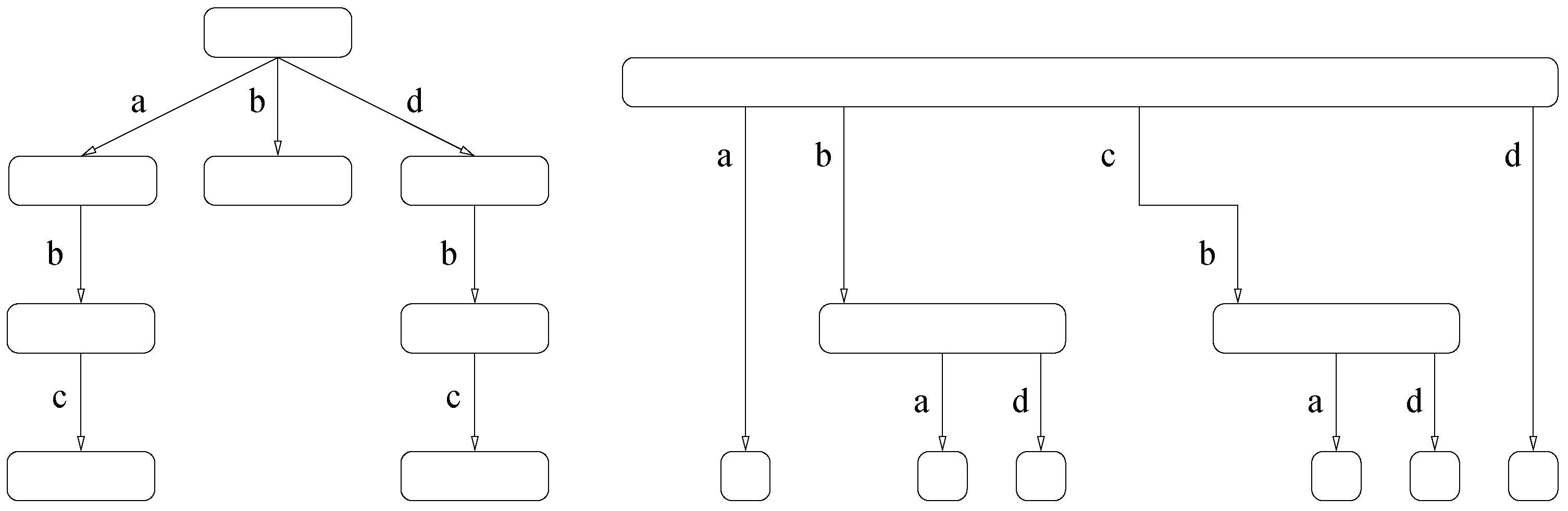
. We show the corresponding LZ-trie in
Figure 3, moreover we also show a tree composed of the reverse phrases which is also an important component of LZ-indexes.
Figure 3.
(left) LZ-trie for strings . (right) Reverse tree of the LZ78 trie.
Figure 3.
(left) LZ-trie for strings . (right) Reverse tree of the LZ78 trie.
The occurrences of a pattern are classified into three categories in the LZ-index. Those of type 1 fall within a single phrase . Those of type 2 span two consecutive phrases, that is, fall within some . Those of type 3 span more than two phrases. Because in a LZ78 parsing all the phrases are different, there are at most occurrences of type 3 overall. Occurrences of type 1 are found by first spotting the type-1 occurrences that lie at the end of their phrase, that is, where P is a suffix of . Let us call those occurrences primary. Primary occurrences are found using other LZ-index structures (in particular, the trie of reverse phrases) in time , plus per primary occurrence found. Now, it turns out that every type-1 occurrence descends from a primary occurrence in the LZ-trie (alternatively, each occurrence where P is inside but not a suffix of it, is inherited from an occurrence of P within the phrase copied by , from which descends in the LZ-trie). Thus all occurrences of type 1 are obtained by simply traversing all LZ-trie subtrees of the primary occurrences. Occurrences of type 2 and 3 are costlier to obtain.
A simple method for ASM is thus to split P into pieces, as evenly as possible, search for those pieces in the LZ-index, extract a context of characters around the occurrence, and run DP over it. This approach will be called LZI in the experiments.
3.2. Improving the Basic Solution
In the sequel we introduce several improvements to the basic approach, to obtain what will be called DLZI in the experiments.
The basic approach carries out redundant work in occurrences of type 1. Assume we are looking for a piece of , . Given an occurrence of it, we must extract text substring of length to the left, and of length to the right of the occurrence , for verification using DP. Consider a primary occurrence at LZ-trie node . To extract the context, we will traverse the upward path from v, so as to obtain the content of . If necessary, we will locate (using other fast LZ-index structures) the node corresponding to , for , and so on, until we have extracted characters. Now we locate to obtain , and so on until extracting characters to the right. Note that, towards the left, we can stop exactly when we have extracted characters, as the phrases are obtained right-to-left, whereas towards the right we must extract complete phrases until exceeding , and then discard the unneeded characters from the last phrase.
As explained, we have to repeat this process for each descendant of v. Let be a child of v by character c. The extraction of from u starts by obtaining c and then repeats exactly the process already carried out for (as ). Our aim is to factor out that redundant work.
Given two strings
S and
X, let us define the
suffix edit distance from
S to
X as
where we note that the formula is not symmetric. Similarly, we define the
prefix edit distance
Note that
is easily computed by traversing
X backwards, whereas
is easier if traversing
X forwards. Now let
be a pattern piece found in the text, so that we have to verify the area
with DP. The occurrence
O minimizing
may start anywhere in
and finish anywhere in
. More precisely, there will be an occurrence within
iff
We factor out the redundant work in the subtree of a primary occurrence as follows. First, we obtain and compute , remembering the last row of the DP matrix (where we have processed and in reverse order, and assuming corresponds to the rows). Indeed, if (where is the text substring corresponding to occurrence v), we only process the last characters of . Otherwise, we obtain the nodes , , and so on until obtaining and computing . If , there is no possible occurrence around v. Otherwise, we obtain and process , , until either we obtain or we process more than characters.
Now we traverse the subtree of
v while avoiding redundant work. We set up a new DP matrix between
and an initially empty string, and traverse the subtree while carrying out a process similar to that described in
Section 2.2. so that, when we are at node
, the matrix corresponds to the edit distance computation between
and
u. Let
be the last row of this matrix upon reaching
u. Now we extract
,
, and so on, so as to compute
starting from
, that is, we avoid reprocessing
u itself. Then we extract
,
, and so on until finding
errors or processing
characters.
3.3. Using the FM-index
A problem when partitioning into
pieces is that some may be much more frequent than others. Since any partitioning into
pieces is good, it is natural to look for the partitioning yielding the least number of verifications to carry out. This can be easily found in time
with (a different) dynamic programming [
16]. However, we need to know the frequencies in the text of every pattern substring. That is, we need to be able of efficiently
counting the number of occurrences of a string.
The LZ-index is not good at this task: It can only count by essentially locating all of the occurrences. We tried some approximate counting methods with no success (more precisely, the final search time decreased, but the time for counting exceeded the gains by far).
Suffix-array based indexes, instead, are very efficient at counting. In particular, we used a variant of the FM-index [
24,
36], which is a self-index that simulates a suffix array within
bits of space. The FM-index can easily count the number of occurrences of all the substrings of
P in
time. Within the same time, the suffix array intervals corresponding to each of the pieces is found. Once the optimal partition is chosen, a context around each occurrence of each of the
pieces is obtained, and DP is run on the context to find the approximate matches.
For the experiments we used an FM-index variant that favors speed over space, described in [
50, Sec. 12.2]. As optimizing the partition did reduce the overall time, we show only this variant in the experiments.
4. An Improved q-samples Index
In this section we extend classical q-sample indexes by allowing samples to overlap the pattern occurrences. This is of interest by itself, and will be used for an irregular sampling index later. Recall that a q-samples index stores the locations, in T, of all the substrings .
4.1. Varying the Error Distribution
We will need to consider parts of samples in the sequel, as well as samples of different lengths. Lemma 1 gives the same number of errors to all the samples, which is disadvantageous when pieces are of different lengths. The next Lemma generalizes Lemma 1 to allow different numbers of errors in each piece.
Lemma 2 Let A and B be strings, let , for strings and some . Let such that . Then there is a substring of B and an i such that .
Proof The edit distance between A and B corresponds to the shortest path in the edit graph of A and B. The partition of A induces a partition in this graph and in particular splits the shortest path. Let be the substring of B that shares the shortest path with . This means that .
Suppose, by absurd, that for every substring of B and every i we have that . Therefore, this is also true for the ’s, i.e. . This is absurd since that way . Therefore, there must exist an i such that . Note that is the substring we mention in the lemma.
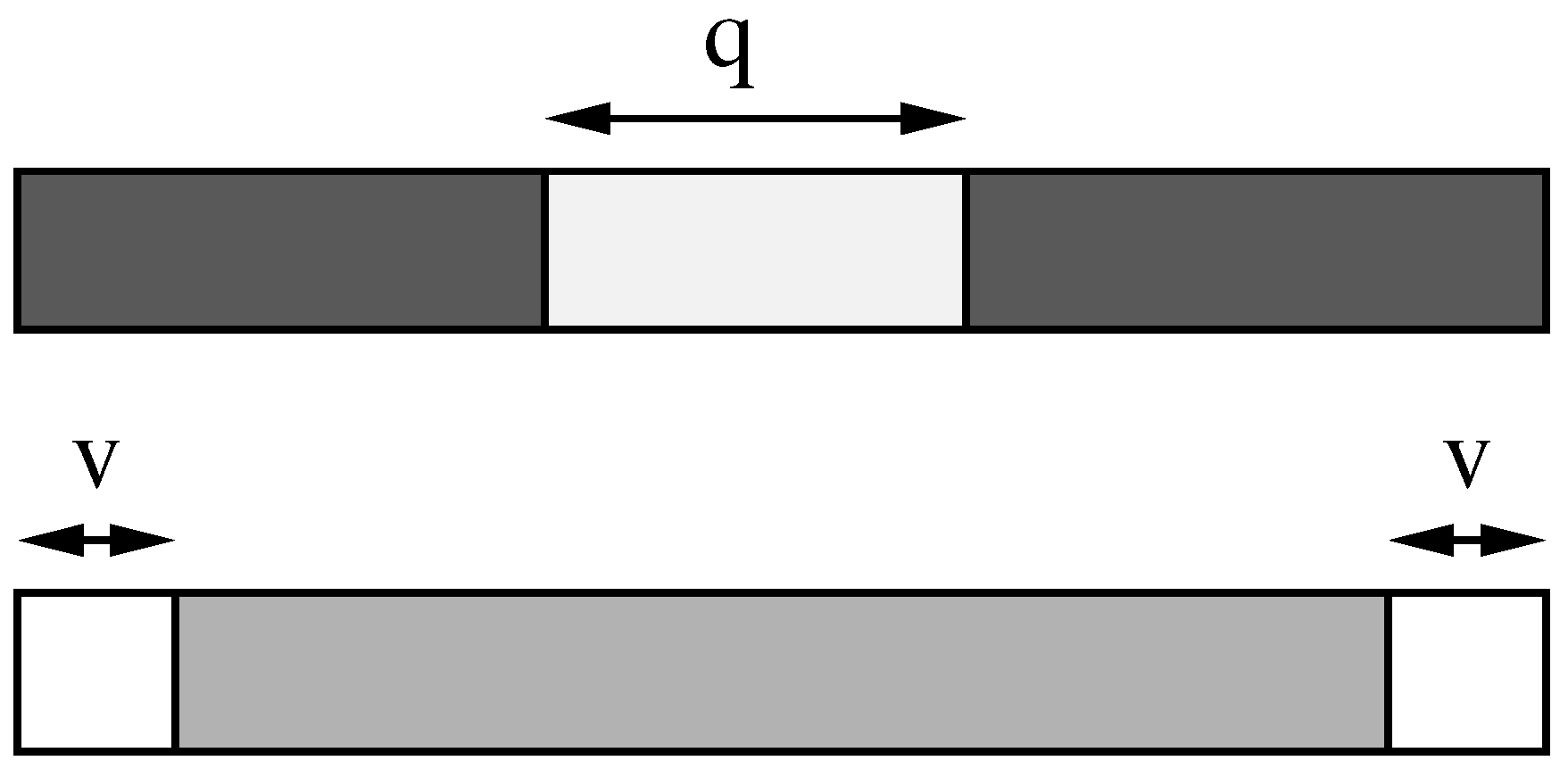
Figure 4 shows an illustration of this Lemma.
Figure 4.
A schematic edit distance graph between A and B. The dashed lines show the division of A and B into the ’s and delimit . The shortest path in the graph is enclosed between two parallel lines.
Figure 4.
A schematic edit distance graph between A and B. The dashed lines show the division of A and B into the ’s and delimit . The shortest path in the graph is enclosed between two parallel lines.
Lemma 1 is a particular case of Lemma 2: set for sufficiently small .
Consider the application of Lemma 1 to
,
,
,
,
and
(see
Figure 5). We can conclude that there is a substring
of
B and an
i such that
. In particular, we have that
and
. This number of errors (3) is excessively high for strings a as small as
and
. Instead, we can use Lemma 2 with
and
; note that
. Using this lemma, we only allow for 1 error for
and
. In this case we have that
. We also have that
.
Figure 5.
Dynamic programming table D for strings, (vertical) and (horizontal) with . The shortest path in the edit graph is shown in bold, we do not show inactive cells.
Figure 5.
Dynamic programming table D for strings, (vertical) and (horizontal) with . The shortest path in the edit graph is shown in bold, we do not show inactive cells.
An early version of Lemma 2 was given in the context of hierarchical verification [
39]. This result was later improved [
4] as follows.
Lemma 3 Let A and B be strings, let , for strings and some . Let such that and . Then there is a substring of B and an i such that .
Proof We will prove this lemma using Lemma 2. Let be the numbers referred in this lemma. Consider . The numbers satisfy the conditions of Lemma 2, i.e. . Therefore, by Lemma 2, we can conclude that there is a substring of B and an i such that . Since and are integers we have that .
The proof shows that Lemma 3 is a consequence of Lemma 2. In fact, both are equivalent. To prove that Lemma 3 implies Lemma 2 use the transformation and reason as above.
In our version the ’s can be real numbers. However, this is not the case of Lemma 3. For example with , and we conclude that some must occur with at most errors. Since the edit distance between two strings is always an integer, the conclusion would be that , which is not correct. With Lemma 2, we can expose our results without being forced to work with integers, i.e. having to deal with floors and ceilings. Also, we do not need to know j a priori, which is important since in our application we will not know the value of j before locating O in T.
Lemma 2 can be used to adapt the error levels to the length of the pieces. For example, it is appropriate to try to maintain a constant error level, by taking for any . In our recent example, this would yield and . This gives essentially the same result we presented before.
4.2. Partial q-sample Matching
Contrary to all previous work, let us assume that A in Lemma 2 is not only that part of an approximate occurrence O formed by full q-samples, but instead that , so that is the suffix of a sample and is the prefix of a sample. An advantage of this is that now the number of involved q-samples is at least , and therefore we can permit fewer errors per piece (e.g., using Lemma 1). On the other hand, we would like to allow fewer errors for the pieces and . Yet, notice that any text q-sample can participate as , , or as a fully contained q-sample in different occurrences at different text positions. Lemma 2 tells us that we could allow errors for , for any . Conservatively, this is for , and less for the extremes.
In order to adapt the trie searching technique to those partial q-samples, we should not only search all the text q-samples with , but also all their prefixes and suffixes with fewer errors. This includes, for example, verifying all the q-samples whose first or last character appears in P (cases and ). This is unaffordable. Our approach will be to redistribute the errors across A using Lemma 2 in a different way to ensure that only sufficiently long q-sample prefixes and suffixes are considered.
Let v be a non-negative integer parameter. We associate to every letter of A a weight: the first and last v letters have weight 0 and the remaining letters have weight . We define as the sum of the weights of the letters of . For example if is within the first v letters of A then ; if it does not contain any of the first or last v letters then . Notice that for this definition to be sound we need that , i.e. .
We can now apply Lemma 2 with provided that . Note that . In this case, if we have that and therefore can never be found with strictly less than zero errors. The same holds for . This effectively relieves us from searching for any q-sample prefix or suffix of length at most v.
Parameter v is thus doing the job of discarding q-samples that have very little overlap with the occurrence , and maintaining the rest. It balances between two exponential costs: one due to verifying all the occurrences of too short prefixes/suffixes, and another due to permitting too many errors when searching for the pieces in the trie. In practice tuning this parameter will have a very significant impact on performance.
Recall the application of Lemma 2 with , , , , , , and . In this case we would need to search for all the q-samples that end in a string that is at edit distance 1 from . This, in particular, includes all the q-samples that contain the suffix a, all the q-samples that contain the suffix b and so on. This yields an excessive number of samples to verify. If we consider in this example we will instead obtain and . Note that . In our example we have that . Note that, in this example, we moved the errors to since and are very small.
4.3. A Hybrid q-samples Index
We have explained all the ideas necessary to describe a hybrid q-samples index. The algorithm works in two steps. First we determine all the q-samples for which for some substring of P. In this phase we also determine the q-samples that contain a suffix for which for some prefix of P (note that we do not need to consider substrings of P, just prefixes). Likewise we also determine the q-samples that contain a prefix for which for some suffix of P (similar observation). The q-samples that qualify are potentially contained inside an approximate occurrence of P, i.e. may be a substring of a string O such that . In order to verify whether this is the case, in the second phase we scan the text context around with a sequential algorithm.
As the reader might have noticed, the problem of verifying conditions such as is that we cannot know a priori which i does a given text q-sample correspond to. Different occurrences of the q-sample in the text could participate in different positions of an O, and even a single occurrence in T could appear in several different O’s. We do not know either the size , as it may range from to .
A simple solution is as follows. Conservatively assume . Then, search P for each different text q-sample in three roles: (1) as a q-sample contained in O, so that , assuming pessimistically ; (2) as an , matching a prefix of P for each of the q-sample suffixes of lengths , assuming and thus ; (3) as an , matching a suffix of P for each of the q-sample prefixes, similarly to case (2) (i.e. ). We assume that and thus the case of O contained inside a q-sample does not occur.
In practice, one does not search for each
q-sample in isolation, but rather factors out the work due to common
q-gram prefixes by backtracking over the trie and incrementally computing the DP matrix between every different
q-sample and any substring of
P ([
4], recall
Section 2.2.). We note that the trie of
q-samples is appropriate for role (3), but not particularly efficient for roles (1) and (2) (finding
q-samples with some specific suffix). In our application to a Lempel-Ziv index this will not be a problem because we will have also a trie of the reversed phrases (that will replace the
q-grams).
5. Using a Lempel-Ziv Self-Index
We now adapt our technique of
Section 4 to the irregular parsing of phrases produced by a Lempel-Ziv-based index. Among the several alternatives [
24,
25,
26,
27,
28], we will focus on the ILZI [
28], for the convenient suffix-tree-like structure of phrases generated. The ILZI partitions the text into phrases such that every suffix of a phrase is also a phrase (similarly to LZ78 parsing [
23], where every prefix of a phrase is also a phrase). It uses two tries, one storing the phrases and another storing the reverse phrases. In addition, it stores a mapping that permits moving from one trie to the other, and it stores the compressed text as a sequence of phrase identifiers. This index [
28] has been shown to require
bits of space, and to be efficient in practice.
5.1. Handling Different Lengths
As explained, the main idea is to use the phrases instead of q-samples. For this sake Lemma 2 solves the problem of distributing the errors homogeneously across phrases. However, other problems arise especially for long phrases. For example, an occurrence could be completely inside a phrase. In general, backtracking over long phrases is too costly.
Even when an occurrence is not completely contained inside a phrase, it is not viable to start searching for an occurrence with too many errors, even if the occurrence is long. This is essentially the argument in favor of filtration and hybrid indexes. Consider our example with , , , , , , and . Recall also that we consider and . It is not viable to search for all the samples such that , by using backtracking. The problem is essentially that, in this way, we allow for all the seven errors to concentrate in the beginning of , i.e. we have to potentially consider for strings. Only a very small fraction of these strings will end up extending to a sample that verifies . To avoid this problem we adopt a hybrid approach.
We resort again to q-samples, this time within phrases. We choose two non-negative integer parameters q and . We will look for any q-gram of P that appears with less than s errors within any phrase. All phrases spotted along this process must be verified. Still, some phrases not containing any pattern q-gram with errors can participate in an occurrence of P (e.g., if or if the phrase is shorter than q). Next we show that those remaining phrases have a certain structure that makes them easy to find.
Lemma 4 Let A and B be strings and q and s be integers such that and for any substrings of B and of A with we have that . Then for every prefix of A there is a substring of B such that .
Proof This is an application of Lemma 2 and it is important because it gives a good description of the restrictions obtained by the filtration.
Apply Lemma 2 with , and the remaining ’s of size q, i.e. . Consider with , . The remaining ’s are equal to s. Note that and therefore .
Therefore we conclude that there is a substring of B and an i such that . We will prove that it must be . If , then , which is impossible. If , then with , which contradicts the hypotheses of the lemma. Therefore and , which means that .
The lemma implies that, if a phrase is close to a substring of P, but none of its q-grams are sufficiently close to any substring of P, then the errors must be distributed uniformly along the phrase. Therefore we can check the phrase progressively (for increasing prefixes), so that the number of errors permitted grows slowly. This severely limits the necessary backtracking to find those phrases that escape from the q-gram-based search.
Let us consider in our running example. Note that for a substring of A of size 4 we have that . Therefore we choose . Note that we cannot use Lemma 4 with and , since and . This means that there is an exceptionally well preserved area of B in A where we only deleted 1 letter out of 5 consecutive ones. Consider instead that and that . In this case we can use Lemma 4 and obtain bound for some substrings of B. Note in particular that this is tight for , i.e. .
Parameter s enables us to balance between two search costs. If we set it low, then the q-gram-based search will be stricter and faster, but the search for the escaping phrases will be costlier. If we set it high, most of the cost will be absorbed by the q-gram search.
5.2. A Hybrid Lempel-Ziv Index
The following lemma describes how we combine previous results to search using a Lempel-Ziv index.
Lemma 5 Let A and B be strings such that . Let , for strings and some . Let q, s and v be integers such that and . Then there is a substring of B and an i such that either:- 1.
there is a substring of with and , or
- 2.
in which case for any prefix of there exists a substring of such that .
Proof As we have explained, our approach first consists in applying Lemma 2 considering for . Observe that, by the definition of , we have that . Now, we classify the resulting into one of the two classes we defined before. The first class justifies the first condition of this Lemma. If the belongs to the second class, we apply Lemma 4 with the resulting .
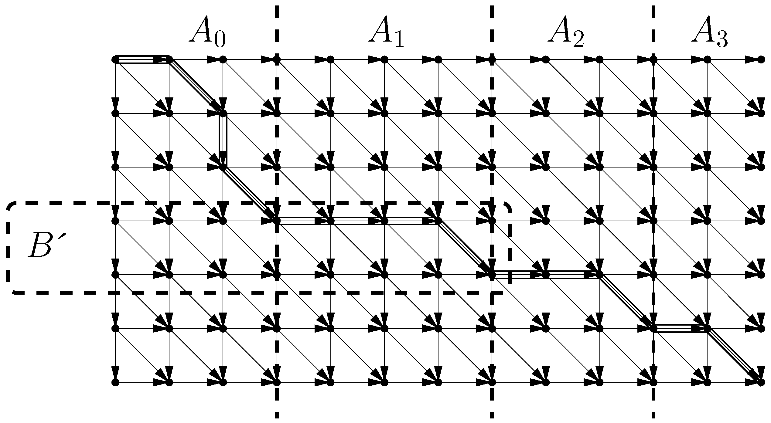
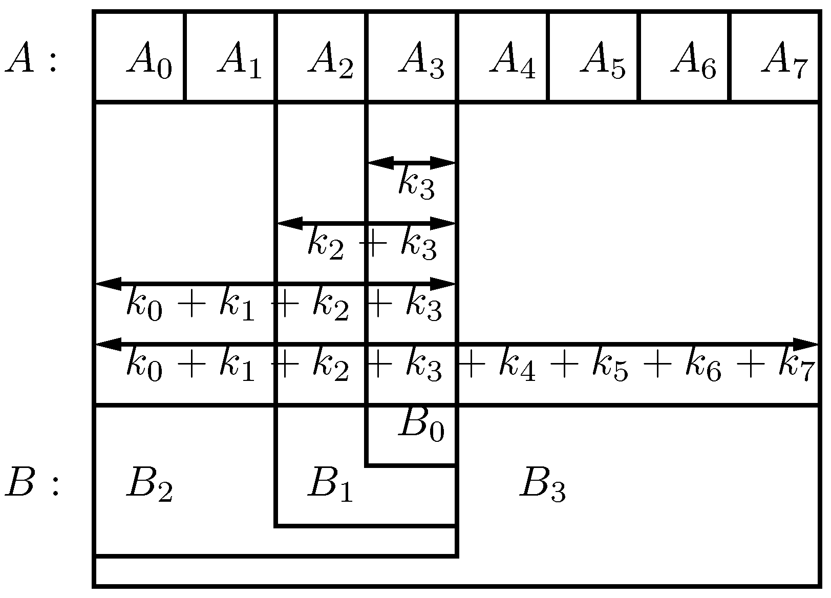
Figure 6 shows a schematic representation of Lemma 5.
As before the search runs in two phases. In the first phase we find the phrases whose text context must be verified. In the second phase we verify those text contexts for an approximate occurrence of P. Lemma 5 gives the key to the first phase. We find the relevant phrases via two searches:
Figure 6.
A schematic representation of the two possible cases mentioned in Lemma 5. The boxes represent the A string and the density of the filling represents the density of errors with B.
Figure 6.
A schematic representation of the two possible cases mentioned in Lemma 5. The boxes represent the A string and the density of the filling represents the density of errors with B.
(1) We look for any q-gram contained in a phrase which matches within P with less than s errors. We backtrack in the trie of phrases for every , descending in the trie and advancing in while computing the DP matrix between the current trie node and . We look for all trie nodes at depth q that match some with less than s errors. Since every suffix of a phrase is a phrase in the ILZI, every q-gram within any phrase can be found starting from the root of the trie of phrases. All the phrases Z that descend from each q-gram trie node found must be verified (those are the phrases that start with that q-gram). We must also spot the phrases suffixed by each such Z. Hence we map each phrase Z to the trie of reverse phrases and also verify all the descent of the reverse trie nodes. This covers case 1 of Lemma 5.
This is precisely the case in our example, since we have that and . We then determine that the phrase contains the string and locate the occurrence by searching the context around that phrase.
(2) We look for any phrase
matching a portion of
P with less than
errors. This is done over the trie of phrases. Yet, as we go down in the trie (thus considering longer phrases), we can enforce that the number of errors found up to depth
d must be less than
. This covers case 2 in Lemma 5, where the equations vary according to the roles described in
Section 4.3. (
i.e. depending on
i):
(2.1) , in which case we are considering a phrase contained inside O that is not a prefix nor a suffix. The formula (both for the matching condition and the backtracking limit) can be bounded by , which depends on . Since may correspond to any trie node that descends from the current one, we determine a priori which maximizes the backtracking limit. We apply the backtracking for each .
This is what occurs in the variation of our example with , that obtains the limit for some substring of . Note that, in particular, this limit is valid for string . Any string for which this is not the case is abandoned by the search.
(2.2) , in which case we are considering a phrase that starts by a suffix of O. Now can be bounded by , yet still the limit depends on and must be maximized a priori. This time we are only interested in suffixes of P, that is, we can perform m searches with and different . If a node verifies the condition we must consider also those that descend from it, to get all the phrases that start with the same suffix.
(2.3) , in which case we are considering a phrase that ends in a prefix of O. This search is as the case , with similar formulas. We are only interested in prefixes of P, that is . As the phrases are suffix-closed, we can conduct a single search for from the trie root, finding all phrase suffixes that match each prefix of P. Each such suffix node must be mapped to the reverse trie and the descent there must be included. The case is different, as it includes the case where O is contained inside a phrase. In this case we do not require the matching trie nodes to be suffixes, but also prefixes of suffixes. That is, we include the descent of the trie nodes and map each node in that descent to the reverse trie, just as in case 1.
5.3. Homogeneous Lempel-Ziv Phrases
In this section we give further insight into the structure of the homogeneous Lempel-Ziv phrases,
i.e. those that verify the conditions of Lemma 4. The objective of this section is to analyze the complexity of the search for the escaping phrases,
i.e. those that are not found in the
q-grams based search. This search for these homogeneous phrases is described in point
(2) of
Section 5.2..
We need a couple of lemmas that give further insight into the structure of these homogeneous phases. Lemma 4 explained that by restricting the minimal number of errors that a substring of A, of size q, may have we are also restricting the maximal number of errors that it can have. In fact this condition also restricts the spacing between consecutive errors. The next lemmas explain this property.
Lemma 6 Let A and B be strings and q and s be integers such that and for any substrings of B and of A with we have that . Then for any prefix of of A such that for any substring of B, we can conclude that , for any .
Proof Suppose by absurd that there is a prefix of A such that for any substring of B we have and for some .
Now apply Lemma 2 with , and the remaining ’s of size q, i.e. and . Consider , and the remaining ’s equal to s. Therefore .
Therefore we conclude that there is a substring of B and an i such that . This, however, is absurd because no value of i may verify this condition. Suppose that . Then , which is impossible. Suppose that . Then with , which contradicts the hypotheses of the lemma. Finally, it cannot be that either. That would mean that for some and this contradicts our initial hypotheses that for any .
Lemma 7 Let A and B be strings and q and s be integers such that and for any substrings of B and of A with we have that . Then for any prefix of of A for which there is a substring of B, we can conclude that , for any .
Proof Suppose by absurd that there is a prefix of A for which there is a substring of B such that and , for some .
Consider the suffix that results from A by removing . Consider also the suffix that results when removing from B. Note that is not necessarily a prefix of B, but we are only interested in the remaining suffix.
We must have , because of the shortest path interpretation. Therefore . The suffix however is too small to contain this number of errors. To see this, apply Lemma 6, replacing 1 by and using and . We conclude that we must have . On the other hand, by our initial hypotheses, we conclude that . Therefore we have reached an absurd condition and the lemma is proved.
Ukkonen studied the structure of the set of
O strings such that
, denoted as
[
51], showing that
. We will now count the number of strings for which the errors are spread homogeneously. We define as
the set of
O strings such that
, and for any substring
of
O, with
, and substring
of
P we have that
.
Lemma 8 .
Proof From the previous lemmas we conclude that, for the strings in
the spacing from an error to the next varies from
to
. Therefore, counting the number of strings in
is a matter of choosing these spacings and the type of error to use. The total number of error types is
. One
σ counts insertions, the other counts substitutions, and the 1 counts the deletions. The number of spacings available is given by the following expression:
Therefore, the number of strings in
can be bounded as follows:
This bound is somewhat loose. In fact, the and never occur together. For example when occurs, the other factor is 1.
We have therefore shown that, by choosing
q and
s properly,
is much smaller than
. Consider for example the optimal case where
. Then
. This shows that the dependence on
m can be reduced to
, which is considerably smaller, especially when we take
. To obtain this optimal result we choose the
q and
s parameters in the same way as in the hybrid index, by using
and
for an appropriate parameter
h. This parameter plays the role of the
j parameter in the classical hybrid index [
52].
6. Hierarchical Approximate String Matching
6.1. Bidirectional Compressed Indexes
Our final algorithm can be implemented over any bidirectional index. This means that, from the index point corresponding to a text substring we can efficiently move to that of but also to that of .
Although classical text indexes are not usually bidirectional, the compressed indexes that simulate suffix arrays are. For example, FM-indexes [
24,
31] offer a so-called LF mapping operation, which moves from the suffix array position
k such that
, to the position
such that
. Compressed suffix arrays [
29,
30,
32], instead, offer function
ψ, which moves to a
such that
, thus
ψ is the inverse of LF. Both kinds of compressed indexes can implement the inverse of their basic functionality, and hence are bidirectional (see [
53] for the case of LF).
The existing compressed suffix trees [
33,
34,
35] build complete suffix tree functionality on top of a compressed suffix array, and hence are bidirectional as well. To fix ideas, let us focus in the so-called
fully compressed suffix trees (FCSTs) [
35], which build on top of an FM-index [
24,
31] and require
bits, although any other combination would essentially fit. The LF mapping of FM-indexes allow FCSTs implement Weiner links [
10]:
WeinerLink, for node
v and letter
a gives the suffix tree node
with path-label
, and it is the key to move from a
v representing
to a
representing
, that is, to bidirectionality. The other direction, that is, from
to
, is supported just by moving to a child of
v. FCSTs support all of the usual suffix tree navigation operations, including suffix links (via
ψ) and lowest common ancestors (
).
Our algorithm will carry out a hybrid search by backtracking on the compressed suffix tree in order to find the approximate occurrences of pattern pieces, yet it will proceed in a slightly more sophisticated fashion. Instead of extending
only in one direction, to the right, we will use a bidirectional search. Landau [
48] obtained the surprising result that it is possible to compute
from
, also in time
. The resulting algorithm is very sophisticated and the reader should consult the original paper. For our purposes all we need are the following observations. (1) The extension is not restricted to
B,
i.e. we can also extend
to
. (2) The number of errors does not have to be fixed,
i.e. we can extend a computation with
k errors to a computation on
errors in
time. (3) Finally, the data structure they use are two doubly linked lists organized in a grid. This means that if we compute
from
we can revert back to the
state by simply keeping a rollback log of which pointers to revert, which requires
computer words (It should be possible to extend their algorithm to support this directly, but if that is not the case we can still use the rollback log idea). For our algorithm this idea suffices since the states we need to visit are always organized in a stack. Thus we never need to compute a sequence such as
to
to
to
.
To improve the success rate of the process described above we should start our search from an area of P that is well preserved. To limit the number of errors we divide the pattern into small pieces. We will use Lemma 2, taking and , and dividing the errors in a homogeneous fashion, i.e. choosing , where and is a number that can be as small as we want and is only used to guarantee that . Recall our running example with and , assuming this is the partition of A. Therefore we should have . Hence the lemma says that in any O there is at least one substring such that or . In our example there are in fact two substrings that satisfy this property, and . This redundancy will make the same string to be found in more than one way. To avoid it, notice that we do not need to add ϵ to both ’s, i.e. we can choose as before and . This means that the conclusion of the lemma now states that there should be an such that or , and hence the redundancy is eliminated.
Note that the condition on is no guarantee that there exists an occurrence O of P, since it is a one-way implication. Hence the area around must be verified to determine whether there is an occurrence or not. Note that in previous work the usual verification procedure is computed on T, not taking advantage of the index. Therefore, verifying those occurrences can cost operations. The problem with dividing P too much, such as when , is that the number of positions to verify can become excessively large and we get a low success rate, i.e. only a small percentage of the s verified by the process turn out to be occurrences of P.
The hybrid approach tries to maximize the overall success rate by finding an optimal balance between filtration and backtracking. It was shown [
52] that the optimal point occurs for
, with a complicated constant. Our approach can have a slightly different optimal point, but if we use their
j the resulting algorithm is never worse than theirs. Moreover we also attempt to automatically determine the optimal point and hence eliminate the need for parameterization.
6.2. Indexed Hierarchical Verification
We modify the verification phase, after filtration, in two ways: (1) We will perform it over the FCST instead of over T, to factor out possibly repeated computations. (2) We use hierarchical instead of direct verification, which also provides a strategy to approximate the optimal point.
The idea of hierarchical verification is to gradually extend the error level instead of jumping directly to k. This is obtained by iterating Lemma 2.
This technique was shown to be extremely efficient for the sequential approach [
52]. We use the following lemma.
Lemma 9 Let A and B be strings, , for strings and some . Let such that . For some fixed , define , for any , as the hierarchical upward path from to A, and define accordingly as the error level corresponding to each . Then there are strings and an i such that for any we have . Moreover, for each , if is a prefix(suffix) of then is a prefix(suffix) of .
Proof For the lemma is trivial because reduces to . To obtain the result for , consider the partition of A into two strings, and (depending on i, either or ), and its edit distance matrix to B achieving edit distance , for and . Then there must be a partition such that or . Thus if (note in this case), and otherwise . To obtain the result for we repeat the process from , , and .
Figure 7 gives a schematic representation of Lemma 9.
Figure 7.
A schematic representation of Lemma 9.
Figure 7.
A schematic representation of Lemma 9.
Consider our running example with
and
. Instead of applying Lemma 9 we will instead iterate Lemma 2, which is actually the way we compute the partition in practice. We divide
into pieces of size 3 and therefore we have
, which in practice means 1 error per piece. Now we divide these pieces as
and we have
and
, which means 0 errors for all the pieces. Notice that we can refine our method by adding
ϵ to only one
, as we did in
Section 2.2.. Hence we can choose
and
and
(and thus
and
). Notice that in our example the occurrence
verifies this Lemma because
and
, where
and
are substrings of
P.
This lemma is used to reduce the cost of verifying an occurrence. Instead of directly verifying the space around a
when
for a string
B such that
, we extend the error level gradually. Assuming
i is even, this means checking for
first, for some
.
Figure 2 (right) shows an example of this process, computed with table
D. Whenever a row reaches a certain level in the hierarchy and contains active cells, the computation on that row is extended to activate the cells that are
. For example since
the cells in row 2 that can be
are activated,
i.e. cells
and
, that correspond to
and
. A similar process happens at row 3. In theory we can compute all the cells that have a value equal or smaller than
k all the time. Still, we can also start to compute them at a given row, especially since it is not necessary to fill upwards the missing cells in the table. That is, we can compute the missing cells, up to
, from the ones already in the table. There is no problem if the value of the new cells is larger than their value on the complete
D table. In fact it is desirable. This will only make the algorithm skip occurrences that, because of Lemma 9, will be found in another case.
To determine that we must compute the D table for these two strings. Extending this computation to is simple because table D only needs to be updated in its natural directions (to the right and downwards). From the suffix tree point of view this situation is also natural because it involves descending in the tree.
When
i is odd the situation is a bit trickier. This time we must check for
. This is much more difficult because we need to move in the FCST by prepending letters to the current point. This is possible with the
WeinerLink operation (recall
Section 6.1.). Moreover we need to extend the DP in unnatural directions (to the left and upwards). For this we use the result [
48] mentioned also in
Section 6.1.. Hence computing each new row requires only
operations. Note that the underlying operation on which their algorithm relies is the longest common prefix of any two suffixes of
A and
B. To solve this we build a FCST for
P, in
time, in uncompressed format so that the LCA operation takes
time. Note that this FCST is built only once at the beginning of the algorithm and adds
bits to the space requirements of the algorithm. We determine the positions of
in that suffix tree, in
time, with the
Parent and
WeinerLink operations. Together with the LCA operation we can compute the size of the necessary longest common prefixes. Note that whenever
is extended to/contracted from
, this information must be updated, by recomputing in
time.
Our algorithm consists in backtracking, where the error bound is gradually increased. Depending on the position of current P’s substring in the hierarchical verification, the string is extended either to the left or to the right. Hence, as mentioned before, the states are stored in a stack, whereas the string being generated is stored in a double stack structure that can be pushed/popped at both ends.
7. Practical Issues and Testing
In this section we present the experimental performance of the algorithms we described in the previous sections. As a baseline we used efficient sequential bit-parallel algorithms (namely BPM, the bit-parallel DP matrix of Myers [
54], and EXP, the exact pattern partitioning by Navarro and Baeza-Yates [
55]). We also used a classical uncompressed hybrid index [
52].
The algorithms of
Section 3. lead to implementations LZI (the basic one, described in
Section 3.1.) and DLZI (the advanced one, described in
Section 3.2.), as well as FMIndex, described in
Section 3.3.. These structures work over the LZ-Index and FM-Index implemented by Navarro [
50], where the second structure is a larger and faster variant of the usual FM-index implementations. Recall that these are pure filtration indexes, using Lemma 1 with
and
, as described in the beginning of
Section 2.3..
The algorithm explained in
Section 4. and
Section 5. is the prototype called ILZI and it is based on the same ILZI compressed index [
28]. For this prototype we used a stricter backtracking than what was explained in previous sections. For each pattern substring
to be matched, we computed the maximum number of errors that could occur when matching it in the text, also depending on the position
where it would be matched, and maximizing over the possible areas of
O where the search would be necessary. For example, the extremes of
P can be matched with fewer errors than the middle. This process involves precomputing tables that depend on
m and
k. We omit the technical details. Note that we could use the ILZI to implement the exact partitioning algorithms run over the LZI and DLZI, yet the ILZI allows for a much stronger search, and we found it more interesting to stress this fact in the experiments.
We also implemented a prototype, BiFMI, to test the algorithm described in
Section 6.. We replaced the FCST with a bidirectional FM-Index over one wavelet tree [
21]. The wavelet tree is a data structure that allows one to compute LF in
time. It contains
σ bitmaps which add up to
bits (that is, the same space of the original text), on which
and
operations are carried out to compute LF and its inverse. We compress these bitmaps using a technique [
56] that solves
/
in constant time and, when applied in the context of an FM-index, achieves
bits of space [
57]. We reverse the search so that the most common search (forwards) is done using LF (where the FM-index is faster) instead of
ψ. Replacing a suffix tree (FCST) by a compressed suffix array (BiFMI) was possible because we did not use the
SLink operation of the FCST.
Note that, since the BiFMI prototype is an FM-Index, it could also have been used to implement the algorithm described in
Section 3.3., instead of the FMIndex structure (The converse is not true, as that FMIndex is intrinsically non-bidirectional. The formula for the inverse of LF [
53] requires an operation called
select that can be carried out efficiently on wavelet-tree-based FM-indexes, but not on this implementation). Yet, the result is in all cases inferior to the hybrid indexing on the BiFMI. On the other hand, the BiFMI cannot reach the speed of the FMIndex for unidirectional search even if using the same amount of space. Thus we found it more interesting to implement the exact partitioning method over the larger and faster FMIndex, to show a different tradeoff.
We tested our algorithm, BiFMI, in
automatic mode,
i.e. Lemma 9 is used until every
. We did not implement the algorithm of Landau [
48]. Instead we used the bit-parallel NFA of Wu [
58] and recomputed the
D table whenever it was necessary to change the computing direction. Note this requires
time when we switch from right to left or vice versa, but after the change it will require only
time for each new row. Although in theory this process could slow down our algorithm by a factor of
, in practice this factor was negligible.
We used the texts from the Pizza&Chili corpus (
http://pizzachili.dcc.uchile.cl), with 50 MB of English and DNA and 64 MB of proteins. The machine was a Pentium 4, 3.2 GHz, 1 MB L2 cache, 1 GB RAM, running Fedora Core 3, and compiling with
gcc-3.4 -O9. The pattern strings were sampled randomly from the text and each character was distorted with
of probability. All the patterns had length
. Every configuration was tested during at least 60 seconds using at least 5 repetitions. Hence the numbers of repetitions varied between 5 and 130,000. To parametrize the hybrid index we tested all the
j values from 1 to
and reported the best time. To parametrize we choose
and
for some convenient
h, since we can prove that this is the best approach and it was corroborated by our experiments. To determine the value of
h and
v we also tested the viable configurations and reported the best results. In our examples choosing
v and
h such that
is slightly smaller than
q yielded the best configuration.
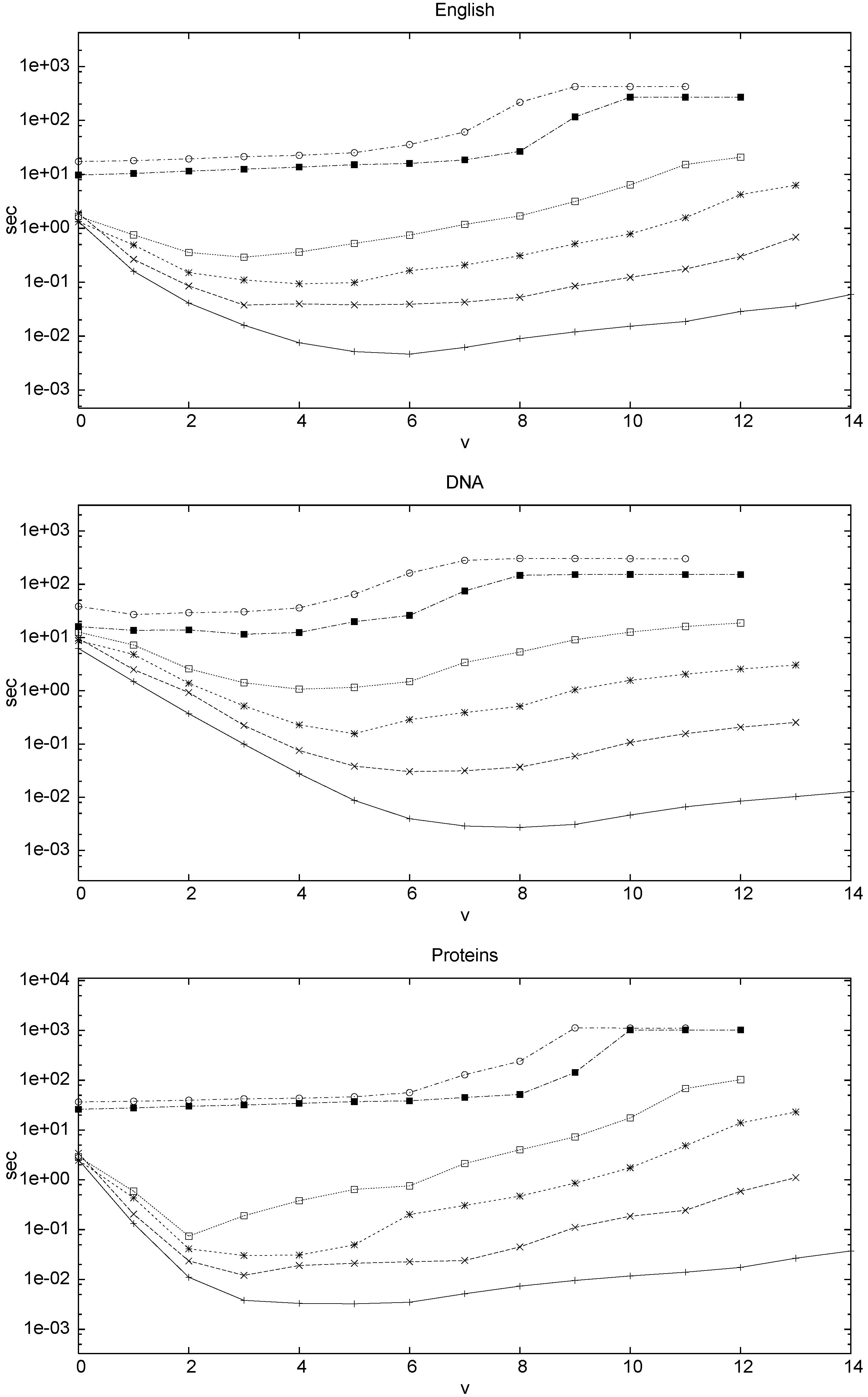
Figure 9 shows the sensitivity of the ILZI to this parameter. The LZI and DLZI are not parametrized.
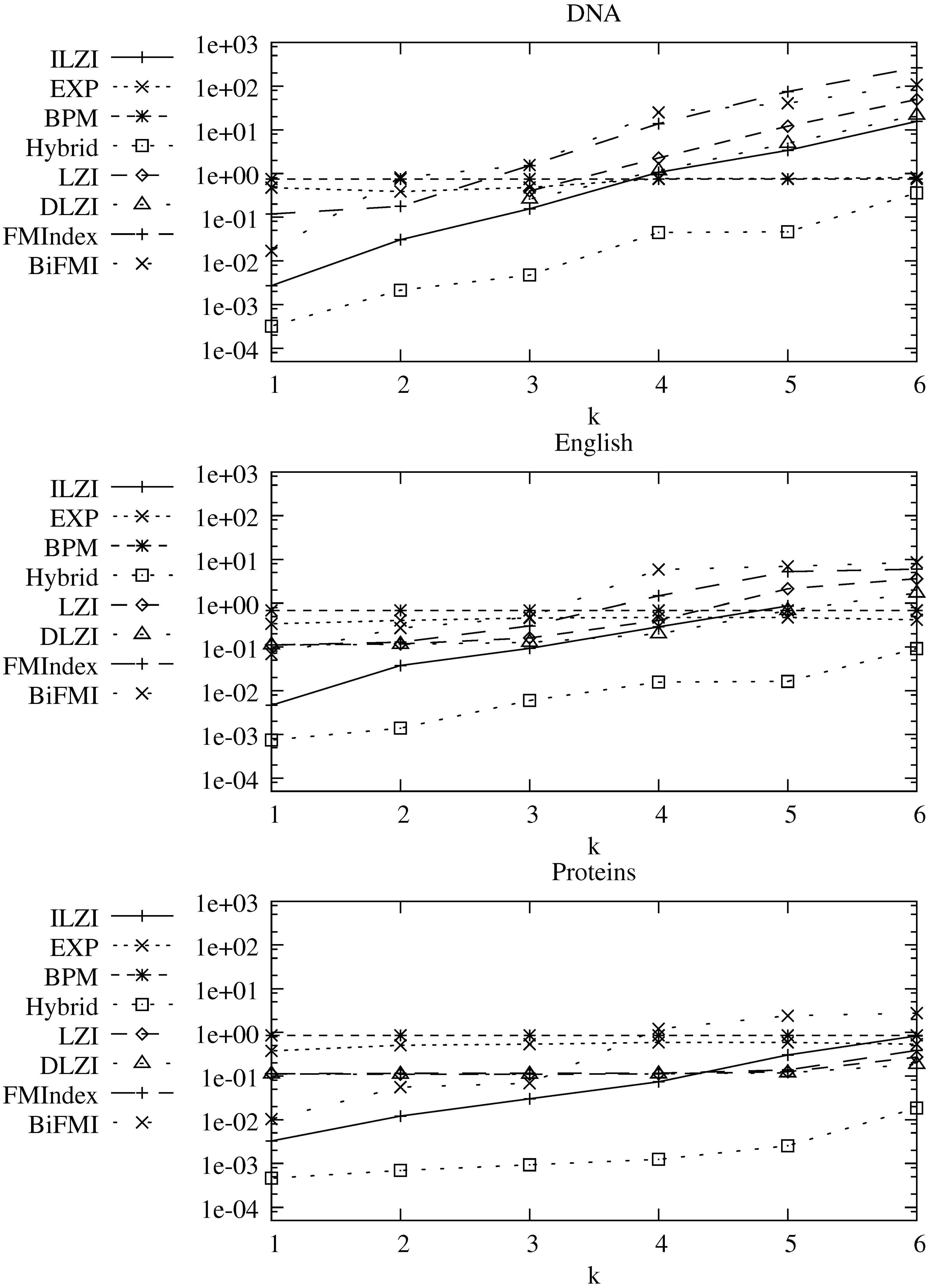
The average query time, in seconds, is shown in
Figure 8, and the respective memory heap peaks for indexed approaches are shown in
Table 1. The hybrid index provides the fastest approach to the problem. However it also requires the most space. Aside from the hybrid index the ILZI is always either the fastest or within reasonable distance from the fastest approach. For low error level,
or
, the ILZI is significantly faster, up to an order of magnitude better. This is very important since this is the area where indexed ASM has chances to make a difference. The sequential approaches outperform all compressed indexing approaches for sufficiently high error levels. In DNA this occurs at
and in English at
.
Figure 8.
Average user time for finding the occurrences of patterns of size 30 with k errors in DNA, English, and Proteins. The y axis units are in seconds.
Figure 8.
Average user time for finding the occurrences of patterns of size 30 with k errors in DNA, English, and Proteins. The y axis units are in seconds.
Figure 9.
Average user time, in seconds, that the ILZI takes to find occurrences of patterns of size 30 with k errors, using different v’s.
Figure 9.
Average user time, in seconds, that the ILZI takes to find occurrences of patterns of size 30 with k errors, using different v’s.
Table 1.
Memory peaks, in Megabytes, for the different approaches when .
Table 1.
Memory peaks, in Megabytes, for the different approaches when .
| | ILZI | Hybrid | LZI | DLZI | FMIndex | BiFMI |
| English | 55 | 257 | 145 | 178 | 131 | 54 |
| DNA | 45 | 252 | 125 | 158 | 127 | 40 |
| Proteins | 105 | 366 | 217 | 228 | 165 | 63 |
The ILZI performed particularly well on proteins, as did the hybrid index. This could be due to the fact that proteins behave closer to random text, and this means that the parametrization of ours and the hybrid index indeed balances between exponential worst cases.
In terms of space the ILZI is also very competitive, as it occupies almost the same space as the plain text, except for proteins. We presented the space that the algorithms need to operate and not just the index size, since the other approaches build intermediate data structures at search time.
Our BiFMI index, on the other hand, achieves the smallest space. We maintain a sparse sampling for our prototype, to show that even within little space we can achieve competitive performance. The FMIndex, on the other hand, needs a much denser sampling to be competitive. Thus our hierarchical and bidirectional verification method is faster than the basic one, even if run on a much slower index.
The performance of the BiFMI prototype closely follows that of ILZI, except for the DNA file. This indicates that it was able to approach hybrid performance in minimal space. It is also, mostly, capable of reducing the gap caused by cache misses.
Among the exact partitioning indexes, the DLZI obtained the best performance. Although it is in some cases the fastest when we exclude Hybrid, in general the compressed hybrid approaches achieved the same or better performance using much less space.
8. Conclusions and Future Work
In this paper we presented two algorithms for ASM in compressed space: an adaptation of the hybrid index for Lempel-Ziv compressed indexes and an hierarchical verification over FCST’s.
We started by addressing the problem of approximate matching with q-samples indexes, where we described a new approach to this problem. We then adapted our algorithm to the irregular parsing produced by Lempel-Ziv indexes. Our approach was flexible enough to be used as a hybrid index instead of an exact-searching-based filtration index. We implemented our algorithm and compared it with the simple filtration approach built over different compressed indexes, with sequential algorithms, and with a good uncompressed index.
Our results show that our index provides a good space-time tradeoff, using a small amount of space (at best
times the text size, which is
times less than a classical index) in exchange for searching from
to 33 times slower than a classical index, for
to 3. This is better than the other compressed approaches for low error levels. This is significant since indexed approaches are most valuable, if compared to sequential approaches, when the error level is low. Therefore our work significantly improves the usability of compressed indexes for approximate matching. A crucial part of our work was our approach for the prefixes/suffixes of
O. This approach is in fact not essential for
q-samples indexes, but it can improve previous approaches [
19]. For a Lempel-Ziv index it is indeed essential.
Our ILZI implementation can be further improved since we do no secondary filtering, that is, we do not apply any sequential filter over the text context before fully verifying them. We also plan to further explore the idea of associating weights to the letters of O. We will investigate the impact of assigning smaller weights to less frequent letters of O. This should decrease the number of positions to verify and improve the overall performance.
We also studied the impact of hierarchical verification in ASM. We obtained an automatic hybrid index that uses fully-compressed suffix trees. This a very important result because it is the first algorithm that approximates the performance of the hybrid index automatically and effectively in practice. Our result is also very important because FCSTs require only compressed space, i.e. bits. Compared with other compressed indexes, our approach was more efficient for low error levels. Although it was less efficient than the ILZI-based algorithm, it requires less space in theory and in practice. In theory, the ILZI requires bits, but in practice that is closer to , including the sublinear term. On the other hand, a FCST requires bits in theory, but this becomes a bit higher in practice if we consider the sublinear term. Moreover our algorithm can be used as a subroutine in a suffix tree algorithm whereas the ILZI-based algorithm cannot.


