
Maximum Entropy Approach to Massive Graph Spectrum Learning with Applications
by
 , and
, and
Diego Granziol
*,† ,
,
Binxin Ru
†,
Xiaowen Dong
,
Stefan Zohren
,
Michael Osborne
and
Stephen Roberts
Machine Learning Research Group, University of Oxford, Eagle House, Walton Well Rd, Oxford OX2 6ED, UK
*
Author to whom correspondence should be addressed.
†
These authors contributed equally to this work.
Algorithms 2022, 15(6), 209; https://doi.org/10.3390/a15060209
Submission received: 30 April 2022
/
Revised: 26 May 2022
/
Accepted: 26 May 2022
/
Published: 15 June 2022
(This article belongs to the Special Issue Extreme Algorithmics: Analysis of Huge, Noisy, and Dynamic Networked Data)
Abstract
:We propose an alternative maximum entropy approach to learning the spectra of massive graphs. In contrast to state-of-the-art Lanczos algorithm for spectral density estimation and applications thereof, our approach does not require kernel smoothing. As the choice of kernel function and associated bandwidth heavily affect the resulting output, our approach mitigates these issues. Furthermore, we prove that kernel smoothing biases the moments of the spectral density. Our approach can be seen as an information-theoretically optimal approach to learning a smooth graph spectral density, which fully respects moment information. The proposed method has a computational cost linear in the number of edges, and hence can be applied even to large networks with millions of nodes. We showcase the approach on problems of graph similarity learning and counting cluster number in the graph, where the proposed method outperforms existing iterative spectral approaches on both synthetic and real-world graphs.
1. Introduction
Many systems of interest can be naturally characterised by complex networks; examples include social networks [1,2,3], biological networks [4] and technological networks. Trends, opinions and ideologies spread on a social network, in which people are nodes and edges represent relationships. Networks are mathematically represented by graphs. Of crucial importance to the understanding of the properties of a network or graph is its spectrum, which is defined as the eigenvalues of its adjacency or Laplacian matrix [5,6]. The spectrum of a graph can be considered as a natural set of graph invariants and has numerous uses including estimating the graph connectivity, e.g., the mixing time on random graphs [7], detecting the presence of specific structures in the graph [8,9,10], graph isomorphism test [11] and measuring graph similarity [12], and graph classification [13]. Practically, it has been extensively studied in the fields of chemistry, physics, computer science and mathematics [14]. One of the main limitations in utilising graph spectra to solve problems such as measuring graph similarity and estimating the number of clusters (these are just two example applications of the general method we propose for learning graph spectra in this paper) is the inability to automatically and consistently learn an everywhere-positive and non-singular approximation to the spectral density. Full eigen-decomposition (which is prohibitive for large graphs) or the Lanczos algorithm both give a Dirac sum that must be smoothed to be everywhere positive. The choice of smoothing kernel and kernel bandwidth choice , or number of histogram bins, which are usually chosen in an ad-hoc manner, can significantly affect the resulting output.
In this paper, we propose a maximum entropy (MaxEnt) approach based on the novel maximum entropy algorithm [15] to learn the spectrum of massive graphs. The main contributions of the paper are as follows:
- We prove that kernel smoothing, commonly used in methods to visualise and compare graph spectral densities, biases moment information;
- We propose a computationally efficient and information-theoretically optimal smooth spectral density approximation based on the method of maximum entropy, which fully respects the moment information. It further admits analytic forms for symmetric and non-symmetric Kullback–Leibler (KL) divergences and Shannon entropy;
- We utilise our information-theoretic spectral density approximation on two example applications. We investigate graph similarity and to learn the number of clusters in a graph, outperforming iterative smoothed spectral approaches on both synthetic and real-world data sets.
2. Graphs and Graph Spectrum
Graphs are the mathematical structure underpinning the formulation of networks. Let be an undirected graph with vertex set . Each edge between two vertices and carries a non-negative weight , the -th entry of the adjacency matrix . For unweighted graphs we set for two connected nodes and 0 for two disconnected nodes. The degree of a vertex is defined as , and the degree matrix is defined as a diagonal matrix that contains the degrees of the vertices along diagonal, i.e., . The unnormalised graph Laplacian matrix is defined as . As G is undirected (), the unnormalised Laplacian is symmetric. As symmetric matrices are special cases of normal matrices, they are Hermitian matrices and have real eigenvalues. Another common variant of the Laplacian matrix is the normalised Laplacian [8],
where is known as the normalised adjacency matrix (strictly speaking the second equality only holds for graphs without isolated vertices). The spectrum of the graph is defined as the density of the eigenvalues of the given adjacency, Laplacian or normalised Laplacian matrices corresponding to the graph. Unless otherwise specified, we will consider the spectrum of the normalised Laplacian.
3. Motivation for a New Method to Approximate and Compare Graph Spectra
For large sparse graphs with millions, or billions, of nodes, learning the exact spectrum using eigen-decomposition is unfeasible due to the cost. Powerful iterative methods (such as the Lanczos algorithm, kernel polynomial methods, Chebyshev/Taylor approximations, the Haydock method and many more), which only require matrix-vector multiplications and hence have a computational cost scaling with the number of non-zero entries in the graph matrices, are often used. There is extensive literature documenting the performance of these methods. Ref. [16] states that the Lanczos algorithm is significantly more accurate than other methods (including the kernel polynomial methods), followed by the Haydock method. Ref. [17] shows that the convergence of the Lanczos algorithm is twice that of the Chebyshev approximation. Hence given the superior theoretical guarantees and empirical performance of the Lanczos algorithm, we employ it as a sole baseline against our MaxEnt method. The Lanczos algorithm [17] approximates the graph spectrum with a sum of weighted Dirac delta functions, closely matching the first m moments (where m is the number of iterative steps used, as detailed in Section 4.1.1) of the spectral density:
where , and denotes the i-th eigenvalue in the spectrum. This can be seen as an m-moment matched discrete approximation to the spectral density of the graph. However, such an approximation is undesirable because natural divergence measures between densities, such as the information-based relative entropy, i.e., the KL divergence [18,19], can be infinite for densities that are mutually singular. The use of the Jensen-Shannon divergence simply re-scales the divergence into .
The Argument against Kernel Smoothing
To alleviate these limitations, practitioners typically generate a smoothed spectral density by convolving the Dirac mixture of spectral components with a smooth kernel [12,20], often a Gaussian or Cauchy [20] to facilitate visualisation and comparison. The smoothed spectral density, with reference to Equation (2), thus takes the form:
We make some assumptions regarding the nature of the kernel function, , in order to prove our main theoretical result about the effect of kernel smoothing on the moments of the underlying spectral density. Both of our assumptions are met by (the commonly employed) Gaussian kernel.
Assumption A1.
The kernel function is supported on the real line .
Assumption A2.
The kernel function is symmetric and permits all moments.
Theorem 1.
The m-th moment of a Dirac mixture , which is smoothed by a kernel satisfying Assumptions 1 and 2, is perturbed from its unsmoothed counterpart by an amount , where if m is even and otherwise. denotes the -th central moment of the kernel function .
Proof.
The moments of the Dirac mixture are given as
The moments of the modified smooth function (Equation (3)) are
We have used the binomial expansion and the fact that the infinite domain is invariant under shift reparameterisation and the odd moments of a symmetric distribution are 0. □
Remark 1.
The above proves that kernel smoothing alters moment information, and that this process becomes more pronounced for higher moments. Furthermore, given that , and (for the normalised Laplacian) , the corrective term is manifestly positive, so the smoothed moment estimates are biased.
Remark 2.
For large random graphs, the moments of a generated instance converge to those averaged over many instances, hence by biasing our moment information we limit our ability to learn about the underlying stochastic process. We include a detailed discussion regarding the relationship between the moments of the graph and the underlying stochastic process in Section 5.2.
Note, of course, that even though our argument here is using the approximate m moment approximation, the same argument would hold if we used the full n-moment information of the underlying matrix (i.e., all the eigenvalues).
4. An Information-Theoretically Optimal Approach to Estimating Massive Graph Spectrum
For large, sparse graphs corresponding to real networks with millions or billions of nodes, where eigen-decomposition is intractable, we may still be able to compute a certain number of matrix-vector products, which we can use to get unbiased estimates of the spectral density moments, using stochastic trace estimation as explained in Section 4.1. We can settle on a unique spectral density which satisfies the given moment information exactly, known as the density of maximum entropy explained in Section 4.2.
4.1. Stochastic Trace Estimation
The intuition behind stochastic trace estimation is that we can accurately approximate the moments of with respect to the spectral density by using computationally cheap matrix-vector multiplications. The moments of can be estimated using a Monte-Carlo average,
where is any random vector with zero mean and unit covariance and is an matrix whose eigenvalues are . This enables us to efficiently estimate the moments in for sparse matrices (where is the number of non-zero entries in the matrix), where . We use these as moment constraints in our entropic graph spectrum formalism to derive the functional form of the spectral density. Examples of this in the literature include [17,21]. The algorithm for learning the graph Laplacian moments is summarised in Algorithm 1.
| Algorithm 1: Learning the Graph Laplacian Moments via Stochastic Trace Estimation (STE). |
|
Comment on the Lanczos Algorithm
In the state-of-the-art iterative algorithm Lanczos [17], the tri-diagonal matrix can be derived from the moment matrix , corresponding to the discrete measure satisfying the moments for all [22] and hence it can be seen as a weighted Dirac approximation to the spectral density matching the first m moments. The weight given on every Ritz eigenvalue (the eigenvalues of the matrix ) is the square of the first component of the corresponding Ritz vector (), i.e., , hence the approximated spectral density can be written as,
As we will further discuss in this paper, whilst this approximate spectral density respects the moment information of the original matrix, in practice as this spectral density is discrete, it must be smoothed. This smoothing neither respects moment nor bound information (for example the matrix may be positive definite). We hence expect a method which respects such information when relevant to provide superior performance, this is the subject of enquiry of this paper.
4.2. Maximum Entropy
The method of maximum entropy, hereafter referred to as MaxEnt, is information-theoretically optimal in so far as it makes the least additional assumptions about the underlying density and is flattest in terms of the KL divergence compared to the uniform [18]. To determine the spectral density using MaxEnt, we maximise the entropic functional
with respect to , where are the power moment constraints on the spectral density, which are estimated using stochastic trace estimation (STE) as explained in Section 4.1. The resultant entropic spectral density has the form
where the coefficients are derived from optimising (8). We use the MaxEnt algorithm, proposed in [15], to learn these coefficients. For simplicity, we denote as . Python code is made available at https://github.com/diegogranziol/Python-MaxEnt accessed on 30 April 2022.
4.3. The Entropic Graph Spectral Learning Algorithm
We first estimate the m moments of the normalised graph Laplacian via STE as shown in Algorithm 1, then use the moment information to solve for MaxEnt coefficients and compute the entropic graph spectrum via Equation (9). The full algorithm for learning the entropic graph spectrum is summarised in Algorithm 2.
| Algorithm 2: Entropic Graph Spectrum (EGS) Learning. |
|
5. Further Remarks
5.1. Analytic Forms for the Differential Entropy and Divergence from EGS
To calculate the differential entropy we simply note that
The KL divergence between two EGSs, and (where refers to the Lagrange multiplier for each moment constraint), can be written as,
where refers to the i-th moment constraint of the density . Similarly, the symmetric-KL divergence can be written as,
where all the and are derived from the optimisation and all the are given from the stochastic trace estimation.
5.2. On the Importance of Moments
Given that all iterative methods essentially generate an m moment empirical spectral density (ESD) approximation, it is instructive to ask what information is contained within the first m spectral moments. To answer this question concretely, we consider the spectra of random graphs. By investigating the finite size corrections and convergence of individual moments of the empirical spectral density (ESD) compared to those of the limiting spectral density (LSD), we see that the observed spectra are faithful to those of the underlying stochastic process. Put simply, given a random graph model, if we compare the moments of the spectral density observed from a single instance of the model to that averaged over many instances, we see that the moments we observe are informative about the underlying stochastic process.
5.2.1. ESD Moments Converge to Those of the LSD
For random graphs, with independent edge creation probabilities, their spectra can be studied through the machinery of random matrix theory [23]. We consider the entries of an matrix to be zero mean and independent, with bounded moments. For such a matrix, a natural scaling which ensures we have a bounded norm as in is . It can be shown (see for instance [24]) that the moments of a particular instance of a random graph and the related random matrix converge to those of the limiting counterpart in probability with a correction of .
5.2.2. Finite Size Corrections to Moments Get Worse with Larger Moments
A key result, akin to the normal distribution for classical densities, is the semicircle law for random matrix spectra [24]. For matrices with independent entries , , with common element-wise bound K, common expectation and variance , and diagonal expectation , it can be shown that the corrections to the semicircle law for the moments of the eigenvalue distribution,
have a corrective factor bounded by [25]
Hence, the finite size effects are larger for higher moments than that for the lower counterparts. This is an interesting result, as it means that for large graphs with , the lowest order moments, which are those learned by any iterative process, best approximate those of the underlying stochastic process.
6. Visualising the Modelling Power of EGS
Having developed a theory as to why a smooth, exact moment-matched approximation of the spectral density is crucial to learning the characteristics of the underlying stochastic process, and having proposed a method (Algorithm 2) to learn such a density, we test the practical utility of our method and algorithm on examples where the limiting spectral density is known.
6.1. Erdős-Rényi Graphs and the Semicircle Law
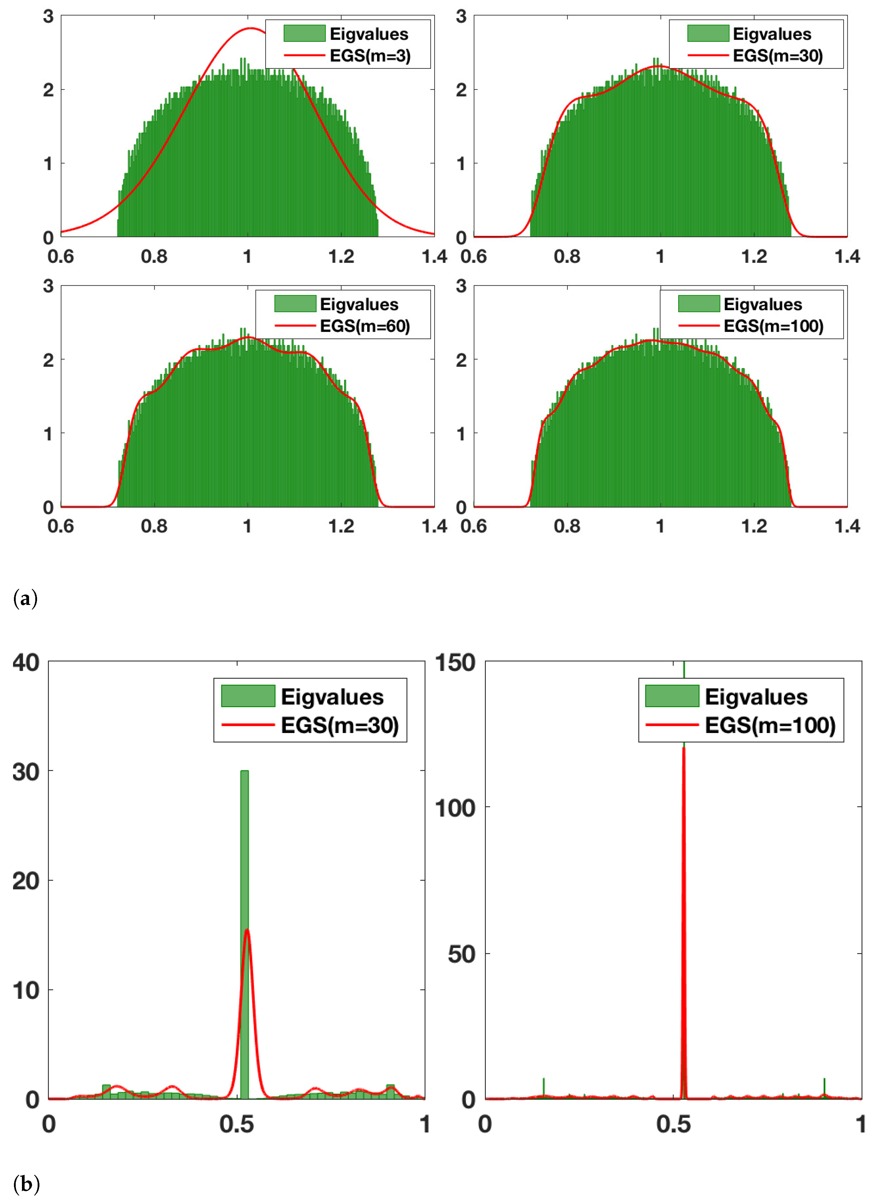
For Erdős-Rényi graphs with n nodes and edge creation probability , and , the limiting spectral density of the normalised Laplacian converges to the semicircle law. We consider here to what extent the learned EGS with finite moments can effectively approximate the density. Wigner’s density is fully defined by its infinite number of central moments given by , where are known as the Catalan numbers. As a toy example we generate a semicircle centered at with and use the analytical moments to compute its corresponding EGS. As can be seen in Figure 1, for moments, the central portion of the density is already well approximated, but the end points are not. This is largely corrected for moments. Next, we generate an Erdős-Rényi graph with and , and learn the moments using stochastic trace estimation. We then compare the fit between the EGS computed using a different numbers of input moments and the graph eigenvalue histogram computed by eigen-decomposition. We plot the results in Figure 2. One striking difference between this experiment and the previous one is the number of moments needed to give a good fit. This can be seen especially clearly in the top left subplot of Figure 2, where using 3 moments, i.e., Gaussian approximation, completely fails to capture the bounded support of the spectral density. Given that the exponential polynomial density is positive everywhere, it needs more moment information to learn the regions of boundedness of the spectral density in its domain. In the previous example we artificially alleviated this phenomenon by putting the support of the semicircle within the entire domain. It can be clearly seen from Figure 2a that increasing moment information successively improves the fit to the support. Furthermore, the magnitude of the oscillations, which are characteristic of an exponential polynomial function, decay for larger moments.
6.2. Beyond the Semicircle Law
For the adjacency matrix of an Erdős-Rényi graph with , the limiting spectral density does not converge to the semicircle law and has an elevated central portion, and the scale-free limiting density converges to a triangle-like distribution. For other random graph models, such as the Barabási-Albert model (also known as the scale-free network), the probability of a new node being connected to a certain existing node is proportional to the number of links that the existing node already has, violating the independence assumption required to derive the semicircle density. We plot a Barabási-Albert network (n = 5000) and, similar to Section 6.1, we learn the EGS and plot the resulting spectral density against the eigenvalue histogram, shown in Figure 2b. For the Barabási-Albert network, due to the extremity of the central peak, a much larger number of moments is required to get a reasonable fit. We also note that increasing the number of moments is akin to increasing the number of bins in terms of spectral resolution, as seen in Figure 2b.
7. EGS for Measuring Graph Similarity
In this section, we test the use of our EGS in combination with symmetric KL divergence to measure similarity between different types of synthetic and real-world graphs. Note that our proposed EGS, based on the MaxEnt distribution, enables the symmetric KL divergence to be computed analytically, which we show in Section 5.1. We first investigate the feasibility of recovering the parameters of random graph models, and then move onto classifying the network type as well as computing graph similarity among various synthetic and real-world graphs.
7.1. Inferring Parameters of Random Graph Models
We investigate whether one can recover parameters of random graph models via the learned EGS of the graph instances. We generate a random graph with a given size and parameters and learn its entropic spectral characterisation using our EGS learner (Algorithm 2). Then, we generate another graph of the same size but learn its parameter value by minimising the symmetric-KL divergence between its entropic spectral surrogate and that of the original graph. We consider three different random graph models, i.e., Erdős-Rényi (ER) with edge probability p, Watts-Strogatz (WS) with rewiring probability p, and Barabási-Albert (BA) with number of edges r attached to each new node, and different graph sizes (). The results are shown in Table 1. It can be seen that, given the approximate EGS, we are able to infer the parameters of the graph producing that spectrum.
7.2. Learning Real-World Network Types
Determining which random graph model best fits a real-world network (characterised by spectral divergence) leads to a better understanding of graph dynamics and characteristics. This has been explored for small biological networks [12] where full eigen-decomposition is viable. Here, we conduct similar experiments (based on our EGS method) for large networks. We first test on a large (5000-node) synthetic BA network. By minimising the symmetric KL divergence between its EGS and those of small (1000-node) random networks (ER, WS, BA), we successfully recover the graph type (see Table 2). As a real-world use case, we further repeat the experiment to determine which random network can best model the YouTube network from the SNAP dataset [26] and find, as shown in Table 2, that the BA gives the lowest divergence. Further we show that EGS can also be used to compare similarity among real-world networks, such as biological, citation and road networks from the SNAP dataset.
7.3. Comparing Different Real-World Networks
We now consider the feasibility of comparing real-world networks using EGS. Specifically, we take 3 biological networks, 5 citation networks and 3 road networks from the SNAP dataset [26], and compute the symmetric KL divergences between their EGS with moments. We present the results in a heat map (Figure 3). We see very clearly that the intra-class divergences between the biological, citation and road networks are much smaller than their inter-class divergences. This strongly suggests that the combination of our EGS method and the symmetric KL divergence can be used to identify similarity in networks. Furthermore, as can be seen in the divergence between the human and mouse network, the spectra of the human gene network are more closely aligned with each other than they are with the spectra of the mouse gene network. This suggests a reasonable amount of intra-class distinguishability as well.
8. EGS for Estimating Cluster Number
It is known from spectral graph theory [10] that the multiplicity of the 0 eigenvalue of the Laplacian (and the normalised Laplacian) is equal to the number of connected components in the graph. For a small number of inter-cluster connections between k clusters, we expect (by matrix perturbation theory) the k smallest eigenvalues to be close to 0. This leads to the so-called eigengap between the k-th and -th eigenvalue which is used as a heuristic to detect number of clusters in a graph [10]. Here, we first make the above argument about eigenvalues precise in the following theorem.
Theorem 2.
The normalised Laplacian eigenvalue, perturbed by adding a single edge between nodes and from two previously disconnected clusters A and B, is bounded to first order by
where denotes the degree of node , and similarly , where denotes the sum over all nodes connecting to node .
Proof.
Using Weyl’s bound on Hermitian matrices
where and are the i-th eigenvalue of the normalised graph Laplacian and for graph G and its perturbed version , respectively, and and denote the matrix 2-norm and Frobenius norm, respectively. By definition that the -th entry of is that of divided by , we have
to first order in the binomial expansion. We hence prove the result. □
Corollary 1.
For two clusters in which nodes have an identical degree , connected by a single inter-cluster link, the zero eigenvalue is perturbed (to first order) by at most .
Remark 3.
For E inter-cluster connections, our bound scales as and hence the intuition of a small change in the 0 eigenvalue holds if the number of edges between clusters is much smaller than the degree of the nodes within the clusters.
For the case of large sparse graphs, where only iterative methods such as the Lanczos algorithm can be used, the same arguments from Section 3 apply. This is because the Dirac delta functions are now weighted, and to obtain a reliable estimate of the eigengap, one must smooth the spectral delta functions. We would expect a smoothed spectral density plot to have a spike near 0, and the moments of the spectral density to encode this information and the mass of this peak to be spread. We hence look for the first spectral minimum in the EGS and calculate the number of clusters as shown in Algorithm 3. We conduct a set of experiments to evaluate the effectiveness of our spectral method in Algorithm 3 for learning the number of clusters in a network, where we compare it against the Lanczos algorithm with kernel smoothing on both synthetic and real-world networks.
| Algorithm 3: Cluster Number Estimation. |
|
8.1. Synthetic Networks
The synthetic data consists of disconnected sub-graphs of varying sizes and cluster numbers, to which a small number of inter-cluster edges are added. We use an identical number of matrix vector multiplications, i.e., (see Section 9 for experimental details for both EGS and Lanczos methods), and estimate the number of clusters and report the fractional error. The results are shown in Table 3. In each case, the method achieving lowest detection error is highlighted in bold. It is evident that the EGS approach outperforms Lanczos as the number of clusters and the network size increase. We observe a general improvement in performance for larger graphs, visible in the differences between fractional errors for EGS as the graph size increases and not for kernel-smoothed Lanczos.
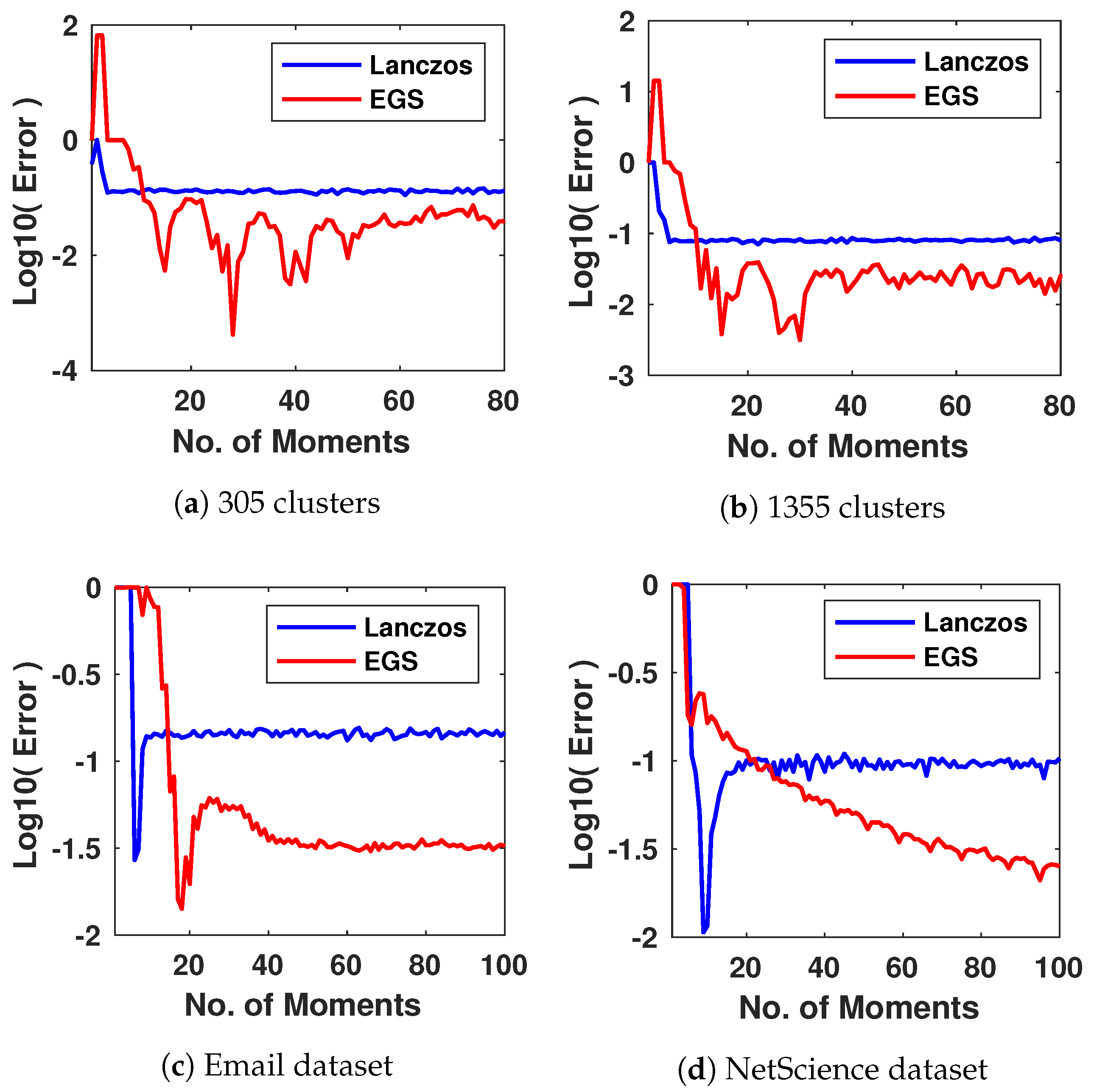
To test the performance of our approach for networks that are too large to apply eigen-decomposition, we generate two large networks by mixing the ER, WA, BA random graph models. The first large network has a size of 201,600 nodes and comprises 305 interconnected clusters whose size varies from 500 to 1000 nodes. The second large network has a size of 404,420 nodes and comprises interconnected 1355 clusters whose size varies from 200 to 400 nodes. The results in Figure 4a,b show that for both methods, the detection error generally decreases as more moments are used, and our EGS approach again outperforms the Lanczos method for both large synthetic networks.
8.2. Small Real-World Networks
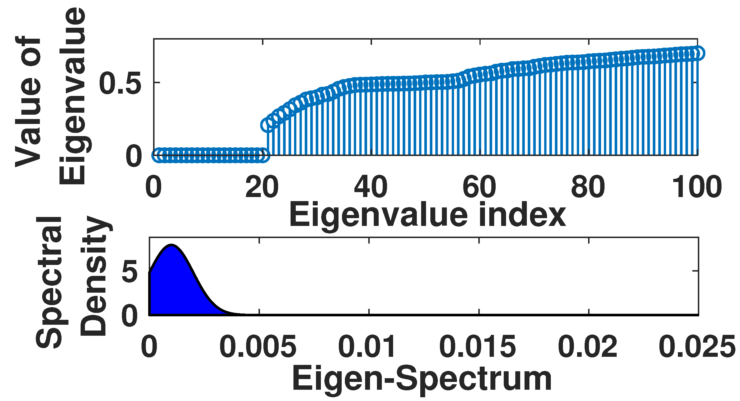
We next experiment with relatively small real-world networks, such as the Email network (with nodes) in the SNAP dataset and the Net Science collaboration network (with nodes) [27]. For such networks, we can still calculate the ground-truth number of clusters by computing the eigenvalues explicitly and finding the spectral gap near 0. For the Email network, we count 20 very small eigenvalues before a large jump in magnitude (measured on a log scale) and set this as the ground-truth (see Figure 5). We plot the log error against the number of moments for both EGS and Lanczos in Figure 4c, with EGS showing superior performance. Similar results have been observed in Figure 4d for the NetScience dataset, which show that EGS quickly outperforms the Lanczos algorithm after around 20 moments.
8.3. Large Real-World Networks
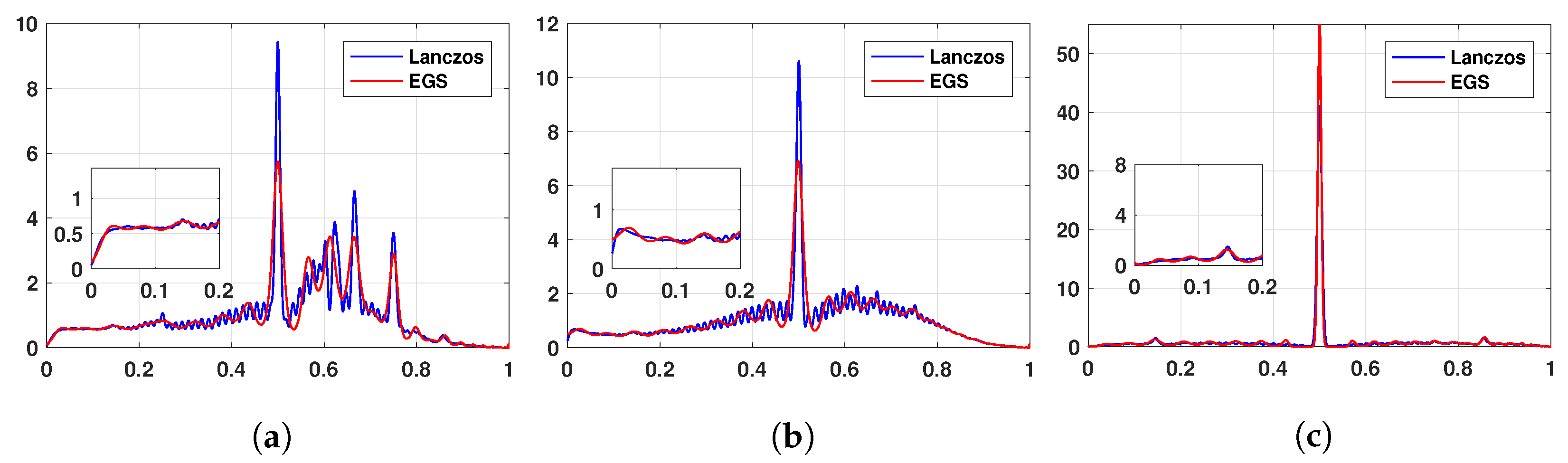
For large datasets with , where the Cholesky decomposition becomes completely prohibitive even for powerful machines, we can no longer define a ground-truth using a complete eigen-decomposition. Nevertheless, we present our findings for the number of clusters in the DBLP (n = 317,080), Amazon (n = 334,863) and YouTube (n = 1,134,890) networks [26] in Table 4, where we use a varying number of moments. We see that for both the DBLP and Amazon networks, the number of clusters seems to converge with increasing moments number m, whereas for YouTube such a trend is not visible. This can be explained by looking at the approximate spectral density of the networks implied by maximum entropy. For both DBLP and Amazon (Figure 6a,b respectively), we see that our method implies a clear spectral gap near the origin, indicating the presence of clusters. Whereas for the YouTube dataset, shown in Figure 6c, no such clear spectral gap is visible and hence the number of clusters cannot be estimated accurately.
9. Experimental Details
We use Gaussian random vectors for our stochastic trace estimation, for both EGS and Lanczos [17]. We explain the procedure of going from adjacency matrix to Laplacian moments in Algorithm 1. When comparing EGS with Lanczos, we set the number of moments m equal to the number of Lanczos steps, as they are both matrix vector multiplications in the Krylov subspace. We further use Chebyshev polynomial input instead of power moments for improved performance and conditioning. In order to normalise the moment input we use the normalised Laplacian with eigenvalues bounded by and divide by 2. To make a fair comparison we take the output from Lanczos [17] and apply kernel smoothing [16] before applying our cluster number estimator.
10. Conclusions
In this paper, we propose a novel, efficient framework for learning a continuous approximation to the spectrum of large-scale graphs, which overcomes the limitations introduced by kernel smoothing. We motivate the informativeness of spectral moments using the link between random graph models and random matrix theory. We show that our algorithm is able to learn the limiting spectral densities of random graph models for which analytical solutions are known. We showcase the strength of this framework in two real-world applications, namely, computing the similarity between different graphs and detecting the number of clusters in the graph. Interestingly, we are able to classify different real-world networks with respect to their similarity to classical random graph models. The EGS may be of further use to researchers studying network properties and similarities.
Author Contributions
D.G. was responsible for the derivation of the maximum entropy algorithm and all the matrix perturbation theory proofs. B.R. assisted with the implementation of the maximum entropy algorithm for massive graphs, conducted several experiments and helped in writing the paper. X.D. and S.Z. identified relevant areas of graph problems that could be solved using the combination of spectral graph theory and maimum entropy. M.O. and S.R. assisted in writing, proof reading the manuscript and checking the soundness of the results. All authors have read and agreed to the published version of the manuscript.
Funding
The lead author is grateful for the financial support provided by the Oxford-Man institute during this work.
Institutional Review Board Statement
Not applicable.
Informed Consent Statement
Not applicable.
Data Availability Statement
Data used in this study were downloaded from http://snap.stanford.edu/data/ accessed on 30 April 2022.
Conflicts of Interest
The authors declare no conflict of interest.
References
- Mislove, A.; Marcon, M.; Gummadi, K.P.; Druschel, P.; Bhattacharjee, B. Measurement and analysis of online social networks. In Proceedings of the 7th ACM SIGCOMM Conference on Internet Measurement, San Diego, CA, USA, 24–26 October 2007; pp. 29–42. [Google Scholar]
- Flake, G.W.; Lawrence, S.; Giles, C.L. Efficient identification of web communities. In Proceedings of the Sixth ACM SIGKDD International Conference on Knowledge Discovery and Data Mining, Boston, MA, USA, 20–23 August 2000; pp. 150–160. [Google Scholar]
- Leskovec, J.; Adamic, L.A.; Huberman, B.A. The dynamics of viral marketing. ACM Trans. Web 2007, 1, 5. [Google Scholar] [CrossRef] [Green Version]
- Palla, G.; Derényi, I.; Farkas, I.; Vicsek, T. Uncovering the overlapping community structure of complex networks in nature and society. Nature 2005, 435, 814. [Google Scholar] [CrossRef] [PubMed] [Green Version]
- Farkas, I.J.; Derényi, I.; Barabási, A.L.; Vicsek, T. Spectra of “real-world” graphs: Beyond the semicircle law. Phys. Rev. E 2001, 64, 026704. [Google Scholar] [CrossRef] [PubMed] [Green Version]
- Cohen-Steiner, D.; Kong, W.; Sohler, C.; Valiant, G. Approximating the Spectrum of a Graph. In Proceedings of the 24th ACM SIGKDD International Conference on Knowledge Discovery & Data Mining, London, UK, 19–23 August 2018; pp. 1263–1271. [Google Scholar]
- Lovász, L. Eigenvalues of Graphs. 2007. Available online: https://web.cs.elte.hu/~lovasz/eigenvals-x.pdf (accessed on 13 June 2022).
- Chung, F.R. Spectral Graph Theory; Number 92; American Mathematical Soc.: Providence, RI, USA, 1997. [Google Scholar]
- Newman, M.E. Modularity and community structure in networks. Proc. Natl. Acad. Sci. USA 2006, 103, 8577–8582. [Google Scholar] [CrossRef] [PubMed] [Green Version]
- Von Luxburg, U. A tutorial on spectral clustering. Stat. Comput. 2007, 17, 395–416. [Google Scholar] [CrossRef]
- Kolla, A.; Koutis, I.; Madan, V.; Sinop, A.K. Spectrally Robust Graph Isomorphism. arXiv 2018, arXiv:1805.00181. [Google Scholar]
- Takahashi, D.Y.; Sato, J.R.; Ferreira, C.E.; Fujita, A. Discriminating different classes of biological networks by analyzing the graphs spectra distribution. PLoS ONE 2012, 7, e49949. [Google Scholar] [CrossRef] [PubMed] [Green Version]
- Pineau, E. Using Laplacian Spectrum as Graph Feature Representation. arXiv 2019, arXiv:1912.00735. [Google Scholar]
- Biggs, N.; Lloyd, E.; Wilson, R. Graph Theory 1736-1936; Oxford University Press: Oxford, UK, 1976. [Google Scholar]
- Granziol, D.; Ru, B.; Zohren, S.; Dong, X.; Osborne, M.; Roberts, S. MEMe: An Accurate Maximum Entropy Method for Efficient Approximations in Large-Scale Machine Learning. Entropy 2019, 21, 551. [Google Scholar] [CrossRef] [PubMed] [Green Version]
- Lin, L.; Saad, Y.; Yang, C. Approximating spectral densities of large matrices. SIAM Rev. 2016, 58, 34–65. [Google Scholar] [CrossRef]
- Ubaru, S.; Chen, J.; Saad, Y. Fast Estimation of tr(f(A)) via Stochastic Lanczos Quadrature. SIAM J. Matrix Anal. Appl. 2017, 38, 1075–1099. [Google Scholar] [CrossRef]
- Cover, T.M.; Thomas, J.A. Elements of Information Theory; John Wiley & Sons: Hoboken, NJ, USA, 2012. [Google Scholar]
- Amari, S.I.; Nagaoka, H. Methods of Information Geometry; American Mathematical Soc.: Providence, RI, USA, 2007; Volume 191. [Google Scholar]
- Banerjee, A. The Spectrum of the Graph Laplacian as a Tool for Analyzing Structure and Evolution of Networks. Ph.D. Thesis, Leipzig University, Leipzig, Germany, 2008. [Google Scholar]
- Fitzsimons, J.; Granziol, D.; Cutajar, K.; Osborne, M.; Filippone, M.; Roberts, S. Entropic Trace Estimates for Log Determinants. In Proceedings of the Joint European Conference on Machine Learning and Knowledge Discovery in Databases, Skopje, Macedonia, 18–22 September 2017; pp. 323–338. [Google Scholar]
- Golub, G.H.; Meurant, G. Matrices, moments and quadrature. In Numerical Analysis 1993; CRC Press: Boca Raton, FL, USA, 1994; Volume 52. [Google Scholar]
- Akemann, G.; Baik, J.; Di Francesco, P. The Oxford Handbook of Random Matrix Theory; Oxford University Press: Oxford, UK, 2011. [Google Scholar]
- Feier, A.R. Methods of Proof in Random Matrix Theory. Ph.D. Thesis, Harvard University, Cambridge, MA, USA, 2012. [Google Scholar]
- Füredi, Z.; Komlós, J. The eigenvalues of random symmetric matrices. Combinatorica 1981, 1, 233–241. [Google Scholar] [CrossRef]
- Leskovec, J.; Krevl, A. SNAP Datasets: Stanford Large Network Dataset Collection. 2014. Available online: http://snap.stanford.edu/data (accessed on 13 June 2022).
- Newman, M.E. Finding community structure in networks using the eigenvectors of matrices. Phys. Rev. E 2006, 74, 036104. [Google Scholar] [CrossRef] [Green Version]
Figure 1.
(a) EGS semicircle fit for different moment number m. (b) KL divergence between semicircle density and EGS.
Figure 1.
(a) EGS semicircle fit for different moment number m. (b) KL divergence between semicircle density and EGS.

Figure 2.
(a) EGS fit to randomly generated Erdős-Rényi graph (, ). The number of moments m used increases from 3 to 100 and the number of bins used for the eigenvalue histogram is . (b) EGS fit to randomly generated Barabási-Albert graph (). The number of moments used for computing EGSs and the number of bins used for the eigenvalue histogram are m = 30, = 50 (Left) and , (Right).

Figure 3.
Symmetric KL heatmap between 9 graphs from the SNAP dataset: (0) bio-human-gene1, (1) bio-human-gene2, (2) bio-mouse-gene, (3) ca-AstroPh, (4) ca-CondMat, (5) ca-GrQc, (6) ca-HepPh, (7) ca-HepTh, (8) roadNet-CA, (9) roadNet-PA, (10) roadNet-TX.
Figure 3.
Symmetric KL heatmap between 9 graphs from the SNAP dataset: (0) bio-human-gene1, (1) bio-human-gene2, (2) bio-mouse-gene, (3) ca-AstroPh, (4) ca-CondMat, (5) ca-GrQc, (6) ca-HepPh, (7) ca-HepTh, (8) roadNet-CA, (9) roadNet-PA, (10) roadNet-TX.

Figure 4.
Log error of cluster number detection using EGS and Lanczos methods on large synthetic networks with (a) 201,600 nodes and 305 clusters and (b) 404,420 nodes and 1355 clusters, and on small-scale real-world networks (c) Email network of 1003 nodes and (d) NetScience network of 1589 nodes.
Figure 4.
Log error of cluster number detection using EGS and Lanczos methods on large synthetic networks with (a) 201,600 nodes and 305 clusters and (b) 404,420 nodes and 1355 clusters, and on small-scale real-world networks (c) Email network of 1003 nodes and (d) NetScience network of 1589 nodes.

Figure 5.
Eigenvalues of the Email dataset with clear spectral gap and . The shaded area multiplied by the number of nodes n predicts the number of clusters.
Figure 5.
Eigenvalues of the Email dataset with clear spectral gap and . The shaded area multiplied by the number of nodes n predicts the number of clusters.

Figure 6.
Spectral density of three large-scale real-world networks estimated by EGS and Lanczos. (a) DBLP dataset, (b) Amazon dataset, (c) YouTube dataset.
Figure 6.
Spectral density of three large-scale real-world networks estimated by EGS and Lanczos. (a) DBLP dataset, (b) Amazon dataset, (c) YouTube dataset.


Table 1.
Average parameters estimated by our MaxEnt-based method for the 3 types of network. The number of nodes in the network is denoted by n.
Table 1.
Average parameters estimated by our MaxEnt-based method for the 3 types of network. The number of nodes in the network is denoted by n.
| n | 50 | 100 | 150 |
|---|---|---|---|
| ER () | |||
| WS () | |||
| BA () |
Table 2.
Minimum KL divergence between the EGSs of random networks and that of a BA graph and YouTube network.
Table 2.
Minimum KL divergence between the EGSs of random networks and that of a BA graph and YouTube network.
| Large BA | YouTube | |
|---|---|---|
| ER | ||
| WS | ||
| BA |
Table 3.
Fractional error in cluster number detection for synthetic networks using EGS and Lanczos methods with 80 moments. denotes the number of clusters in the network and the number of nodes. Best results given in bold font.
Table 3.
Fractional error in cluster number detection for synthetic networks using EGS and Lanczos methods with 80 moments. denotes the number of clusters in the network and the number of nodes. Best results given in bold font.
| 9 | 30 | 90 | 240 | |
|---|---|---|---|---|
| Lanc | ||||
| EGS |
Table 4.
Cluster number detection by EGS in the DBLP (n = 317,080), Amazon (n = 334,863) and YouTube (n = 1,134,890) datasets.
Table 4.
Cluster number detection by EGS in the DBLP (n = 317,080), Amazon (n = 334,863) and YouTube (n = 1,134,890) datasets.
| Moments | 40 | 70 | 100 |
|---|---|---|---|
| DBLP | |||
| Amazon | |||
| Youtube |
Publisher’s Note: MDPI stays neutral with regard to jurisdictional claims in published maps and institutional affiliations. |
© 2022 by the authors. Licensee MDPI, Basel, Switzerland. This article is an open access article distributed under the terms and conditions of the Creative Commons Attribution (CC BY) license (https://creativecommons.org/licenses/by/4.0/).
Share and Cite
MDPI and ACS Style
Granziol, D.; Ru, B.; Dong, X.; Zohren, S.; Osborne, M.; Roberts, S. Maximum Entropy Approach to Massive Graph Spectrum Learning with Applications. Algorithms 2022, 15, 209. https://doi.org/10.3390/a15060209
AMA Style
Granziol D, Ru B, Dong X, Zohren S, Osborne M, Roberts S. Maximum Entropy Approach to Massive Graph Spectrum Learning with Applications. Algorithms. 2022; 15(6):209. https://doi.org/10.3390/a15060209
Chicago/Turabian StyleGranziol, Diego, Binxin Ru, Xiaowen Dong, Stefan Zohren, Michael Osborne, and Stephen Roberts. 2022. "Maximum Entropy Approach to Massive Graph Spectrum Learning with Applications" Algorithms 15, no. 6: 209. https://doi.org/10.3390/a15060209
Note that from the first issue of 2016, this journal uses article numbers instead of page numbers. See further details here.