
Using Explainable Machine Learning to Explore the Impact of Synoptic Reporting on Prostate Cancer

 , , ,
, , ,
Abstract
:1. Introduction
Synoptic Reporting
2. Materials and Methods
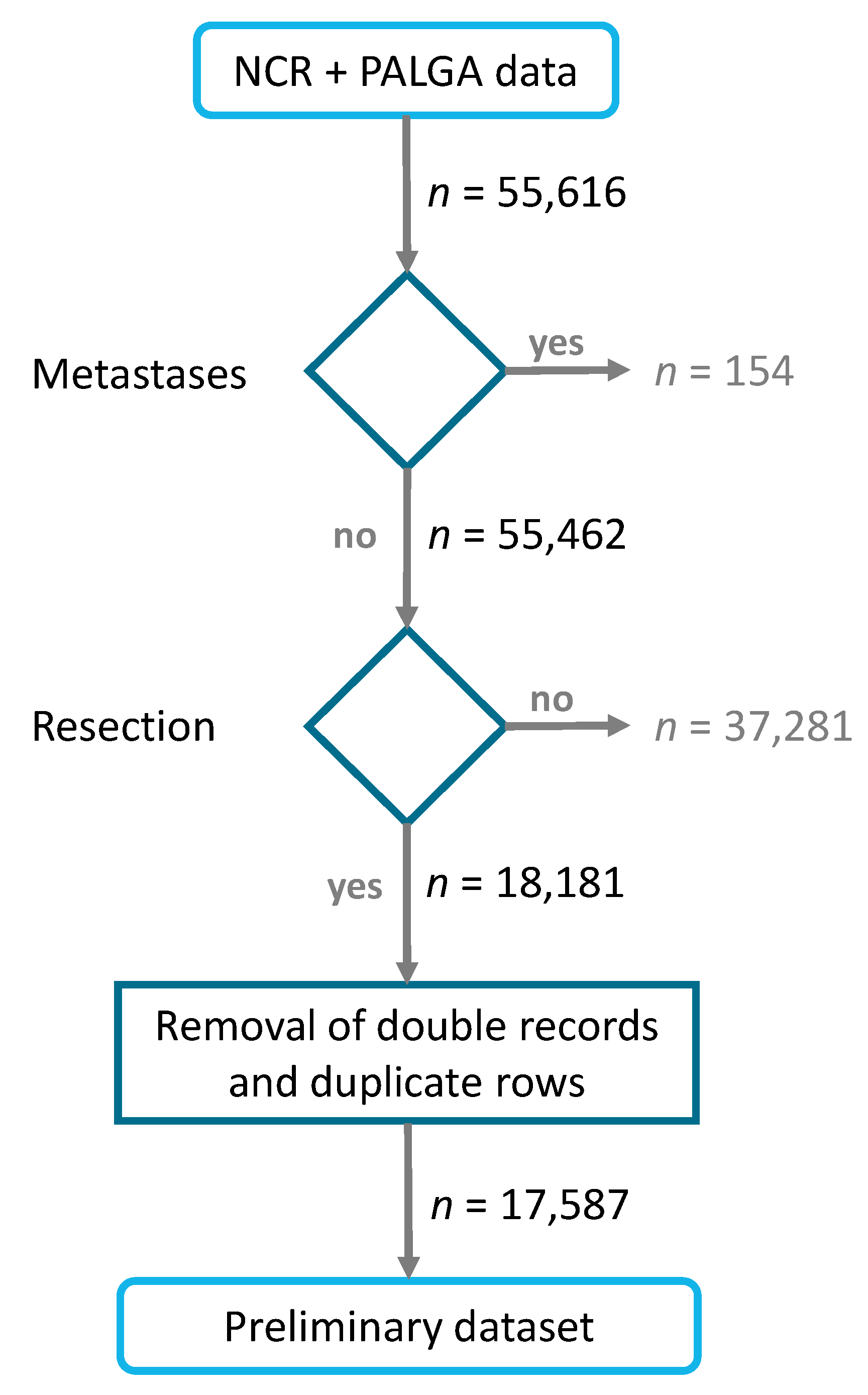
2.1. Data
2.2. Pre-Processing
2.2.1. Feature Engineering
2.2.2. Feature Selection
2.2.3. Dealing with Missing Values
2.3. Models
2.3.1. Model Evaluation
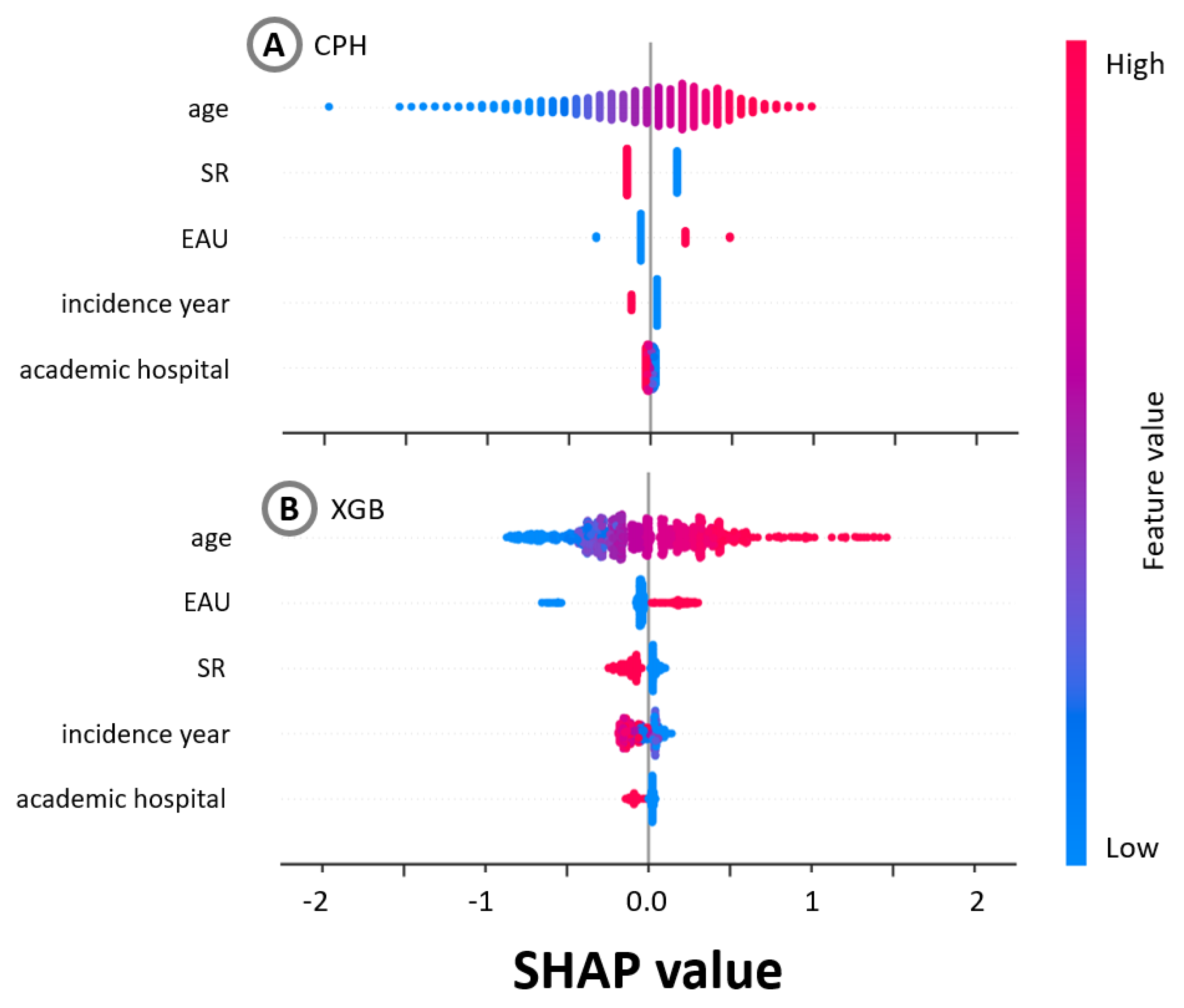
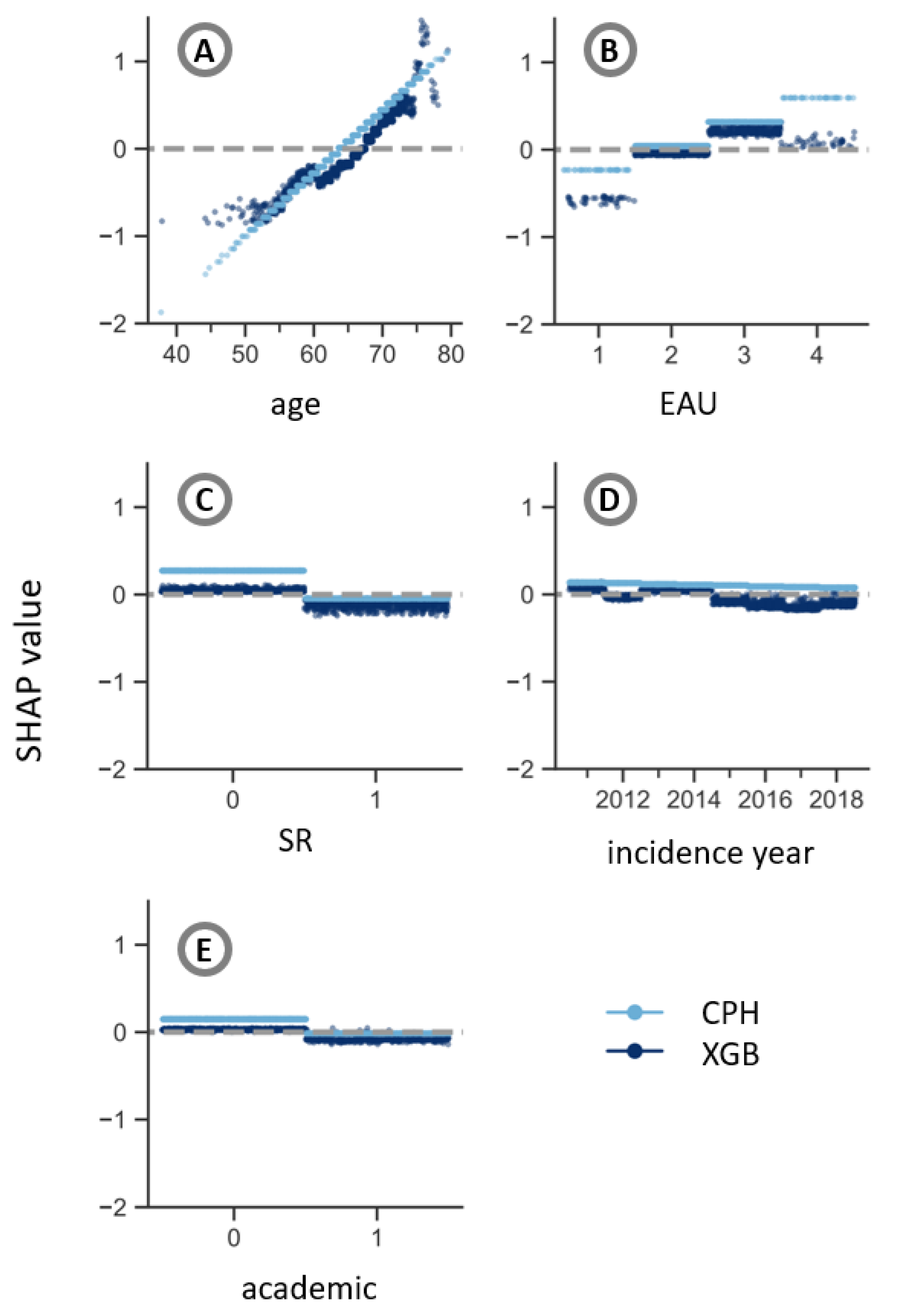
2.4. Explainability
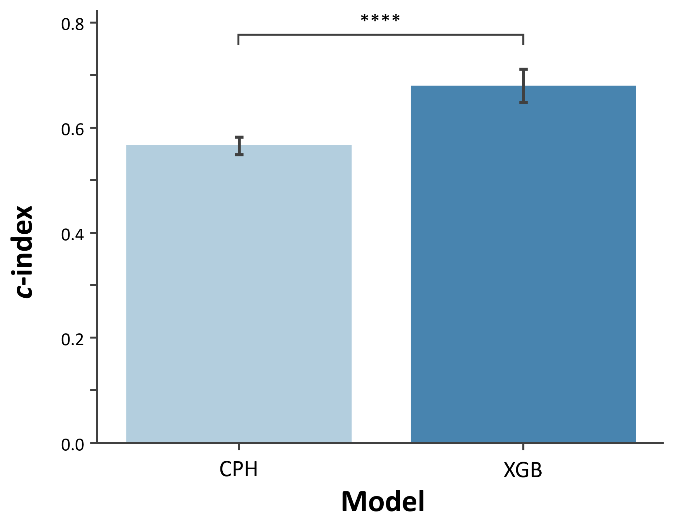
3. Results
4. Discussion
5. Conclusions
Author Contributions
Funding
Institutional Review Board Statement
Informed Consent Statement
Data Availability Statement
Acknowledgments
Conflicts of Interest
Abbreviations
| CPH | Cox Proportional Hazards |
| EAU | European Association of Urology risk group |
| GS | Gleason score |
| HR | Hazard ratio |
| LIME | Local Interpretable Model-agnostic Explanations |
| NCR | Netherlands Cancer Registry |
| NLP | Natural Language Processing |
| PALGA | Nationwide Network and Registry of Histo- and Cytopathology in the Netherlands |
| PSA | Prostate-specific antigen |
| SD | Standard deviation |
| SHAP | SHapley Additive exPlanations |
| SR | Synoptic Reporting |
| TNM | Tumor, nodes, metastases |
| UICC | Union for International Cancer Control |
| XGB | eXtreme Gradient Boosting |
References
- Ravì, D.; Wong, C.; Deligianni, F.; Berthelot, M.; Andreu-Perez, J.; Lo, B.; Yang, G.Z. Deep learning for health informatics. IEEE J. Biomed. Health Inform. 2016, 21, 4–21. [Google Scholar] [CrossRef] [PubMed] [Green Version]
- Panch, T.; Szolovits, P.; Atun, R. Artificial intelligence, machine learning and health systems. J. Glob. Health 2018, 8, 020303. [Google Scholar] [CrossRef] [PubMed]
- Ghassemi, M.; Naumann, T.; Schulam, P.; Beam, A.L.; Chen, I.Y.; Ranganath, R. A review of challenges and opportunities in machine learning for health. AMIA Summits Transl. Sci. Proc. 2020, 2020, 191. [Google Scholar] [PubMed]
- Kourou, K.; Exarchos, T.P.; Exarchos, K.P.; Karamouzis, M.V.; Fotiadis, D.I. Machine learning applications in cancer prognosis and prediction. Comput. Struct. Biotechnol. J. 2015, 13, 8–17. [Google Scholar] [CrossRef] [Green Version]
- Cuocolo, R.; Caruso, M.; Perillo, T.; Ugga, L.; Petretta, M. Machine Learning in oncology: A clinical appraisal. Cancer Lett. 2020, 481, 55–62. [Google Scholar] [CrossRef]
- Ngiam, K.Y.; Khor, W. Big data and machine learning algorithms for health-care delivery. Lancet Oncol. 2019, 20, e262–e273. [Google Scholar] [CrossRef]
- Munir, K.; Elahi, H.; Ayub, A.; Frezza, F.; Rizzi, A. Cancer Diagnosis Using Deep Learning: A Bibliographic Review. Cancers 2019, 11, 1235. [Google Scholar] [CrossRef] [Green Version]
- Wang, P.; Li, Y.; Reddy, C.K. Machine learning for survival analysis: A survey. ACM Comput. Surv. 2019, 51, 1–36. [Google Scholar] [CrossRef]
- Bou-Hamad, I.; Larocque, D.; Ben-Ameur, H. A review of survival trees. Stat. Surv. 2011, 5, 44–71. [Google Scholar] [CrossRef]
- Raftery, A.E.; Madigan, D.; Volinsky, C.T. Accounting for model uncertainty in survival analysis improves predictive performance. Bayesian Stat. 1996, 5, 323–349. [Google Scholar]
- Pölsterl, S.; Navab, N.; Katouzian, A. Fast training of support vector machines for survival analysis. In Proceedings of the Joint European Conference on Machine Learning and Knowledge Discovery in Databases, Porto, Portugal, 7–11 September 2015; pp. 243–259. [Google Scholar]
- Katzman, J.L.; Shaham, U.; Cloninger, A.; Bates, J.; Jiang, T.; Kluger, Y. DeepSurv: Personalized treatment recommender system using a Cox proportional hazards deep neural network. BMC Med. Res. Methodol. 2018, 18, 24. [Google Scholar] [CrossRef] [PubMed]
- Ishwaran, H.; Kogalur, U.B.; Blackstone, E.H.; Lauer, M.S. Random survival forests. Ann. Appl. Stat. 2008, 2, 841–860. [Google Scholar] [CrossRef]
- Chen, T.; Guestrin, C. XGBoost: A Scalable Tree Boosting System. In Proceedings of the 22nd ACM SIGKDD International Conference on Knowledge Discovery and Data Mining, San Francisco, CA, USA, 13–17 August 2016; pp. 785–794. [Google Scholar] [CrossRef] [Green Version]
- Duval, A. Explainable Artificial Intelligence (XAI); Mathematics Institute, The University of Warwick: Coventry, UK, 2019. [Google Scholar]
- Ribeiro, M.T.; Singh, S.; Guestrin, C. Why should I trust you? Explaining the Predictions of Any Classifier. arXiv 2016, arXiv:1602.04938. [Google Scholar]
- Doshi-Velez, F.; Kim, B. Towards a rigorous science of interpretable machine learning. arXiv 2017, arXiv:1702.08608. [Google Scholar]
- Holzinger, A.; Biemann, C.; Pattichis, C.S.; Kell, D.B. What do we need to build explainable AI systems for the medical domain? arXiv 2017, arXiv:1712.09923. [Google Scholar]
- Altmann, A.; Toloşi, L.; Sander, O.; Lengauer, T. Permutation importance: A corrected feature importance measure. Bioinformatics 2010, 26, 1340–1347. [Google Scholar] [CrossRef]
- Apley, D.W.; Zhu, J. Visualizing the effects of predictor variables in black box supervised learning models. J. R. Stat. Soc. Ser. B 2020, 82, 1059–1086. [Google Scholar] [CrossRef]
- Lundberg, S.M.; Lee, S.I. A unified approach to interpreting model predictions. Adv. Neural Inf. Process. Syst. 2017, 2017, 4765–4774. [Google Scholar]
- Guidotti, R.; Monreale, A.; Ruggieri, S.; Turini, F.; Giannotti, F.; Pedreschi, D. A Survey of Methods for Explaining Black Box Models. ACM Comput. Surv. 2018, 51, 93:1–93:42. [Google Scholar] [CrossRef] [Green Version]
- Adadi, A.; Berrada, M. Peeking inside the black-box: A survey on Explainable Artificial Intelligence (XAI). IEEE Access 2018, 6, 52138–52160. [Google Scholar] [CrossRef]
- Ahmad, M.A.; Eckert, C.; Teredesai, A. Interpretable machine learning in healthcare. In Proceedings of the 2018 ACM International Conference on Bioinformatics, Computational Biology, and Health Informatics, Washington, DC, USA, 29 August–1 September 2018; pp. 559–560. [Google Scholar]
- Pawar, U.; O’Shea, D.; Rea, S.; O’Reilly, R. Explainable ai in healthcare. In Proceedings of the 2020 International Conference on Cyber Situational Awareness, Data Analytics and Assessment (CyberSA), Dublin, Ireland, 15–19 June 2020; pp. 1–2. [Google Scholar]
- Tonekaboni, S.; Joshi, S.; McCradden, M.D.; Goldenberg, A. What clinicians want: Contextualizing explainable machine learning for clinical end use. In Proceedings of the Machine Learning for Healthcare Conference, PMLR, Ann Arbor, MI, USA, 9–10 August 2019; pp. 359–380. [Google Scholar]
- Okagbue, H.I.; Adamu, P.I.; Oguntunde, P.E.; Obasi, E.C.M.; Odetunmibi, O.A. Machine learning prediction of breast cancer survival using age, sex, length of stay, mode of diagnosis and location of cancer. Health Technol. 2021, 11, 887–893. [Google Scholar] [CrossRef]
- Moncada-Torres, A.; van Maaren, M.C.; Hendriks, M.P.; Siesling, S.; Geleijnse, G. Explainable machine learning can outperform Cox regression predictions and provide insights in breast cancer survival. Sci. Rep. 2021, 11, 6968. [Google Scholar] [CrossRef]
- Li, R.; Shinde, A.; Liu, A.; Glaser, S.; Lyou, Y.; Yuh, B.; Wong, J.; Amini, A. Machine Learning-Based Interpretation and Visualization of Nonlinear Interactions in Prostate Cancer Survival. JCO Clin. Cancer Inform. 2020, 4, 637–646. [Google Scholar] [CrossRef] [PubMed]
- Giraud, P.; Giraud, P.; Nicolas, E.; Boisselier, P.; Alfonsi, M.; Rives, M.; Bardet, E.; Calugaru, V.; Noel, G.; Chajon, E.; et al. Interpretable Machine Learning Model for Locoregional Relapse Prediction in Oropharyngeal Cancers. Cancers 2021, 13, 57. [Google Scholar] [CrossRef] [PubMed]
- Jansen, T.; Geleijnse, G.; van Maaren, M.; Hendriks, M.P.; Ten Teije, A.; Moncada-Torres, A. Machine Learning Explainability in Breast Cancer Survival. In Studies in Health Technology and Informatics. Digital Personalized Health and Medicine; IOS Press: Amsterdam, The Netherlands, 2020; Volume 270, pp. 307–311. [Google Scholar]
- Valenstein, P.N. Formatting pathology reports: Applying four design principles to improve communication and patient safety. Arch. Pathol. Lab. Med. 2008, 132, 84–94. [Google Scholar] [CrossRef] [PubMed]
- Aumann, K.; Niermann, K.; Asberger, J.; Wellner, U.; Bronsert, P.; Erbes, T.; Hauschke, D.; Stickeler, E.; Gitsch, G.; Kayser, G.; et al. Structured reporting ensures complete content and quick detection of essential data in pathology reports of oncological breast resection specimens. Breast Cancer Res. Treat. 2016, 156, 495–500. [Google Scholar] [CrossRef] [PubMed]
- Nakhleh, R.E. Quality in surgical pathology communication and reporting. Arch. Pathol. Lab. Med. 2011, 135, 1394–1397. [Google Scholar] [CrossRef] [Green Version]
- Sluijter, C.E.; van Workum, F.; Wiggers, T.; van de Water, C.; Visser, O.; van Slooten, H.J.; Overbeek, L.I.H.; Nagtegaal, I.D. Improvement of Care in Patients With Colorectal Cancer: Influence of the Introduction of Standardized Structured Reporting for Pathology. JCO Clin. Cancer Inform. 2019, 3, 1–12. [Google Scholar] [CrossRef] [PubMed] [Green Version]
- Powsner, S.M.; Costa, J.; Homer, R.J. Clinicians are from Mars and pathologists are from Venus. Arch. Pathol. Lab. Med. 2000, 124, 1040–1046. [Google Scholar] [CrossRef] [PubMed]
- Leslie, K.O.; Rosai, J. Standardization of the surgical pathology report: Formats, templates, and synoptic reports. Semin. Diagn. Pathol. 1994, 11, 253–257. [Google Scholar] [PubMed]
- Williams, C.L.; Bjugn, R.; Hassell, L. Current status of discrete data capture in synoptic surgical pathology and cancer reporting. Pathol. Lab. Med. Int. 2015. [Google Scholar] [CrossRef] [Green Version]
- Ellis, D.W. Surgical pathology reporting at the crossroads: Beyond synoptic reporting. Pathology 2011, 43, 404–409. [Google Scholar] [CrossRef] [PubMed]
- Ellis, D.W.; Srigley, J. Does standardised structured reporting contribute to quality in diagnostic pathology? The importance of evidence-based datasets. Virchows Arch. Int. J. Pathol. 2016, 468, 51–59. [Google Scholar] [CrossRef] [PubMed]
- Qu, Z.; Ninan, S.; Almosa, A.; Chang, K.G.; Kuruvilla, S.; Nguyen, N. Synoptic reporting in tumor pathology: Advantages of a web-based system. Am. J. Clin. Pathol. 2007, 127, 898–903. [Google Scholar] [CrossRef] [Green Version]
- Baranov, N.S.; Nagtegaal, I.D.; van Grieken, N.C.T.; Verhoeven, R.H.A.; Voorham, Q.J.M.; Rosman, C.; van der Post, R.S. Synoptic reporting increases quality of upper gastrointestinal cancer pathology reports. Virchows Arch. 2019, 475, 255–259. [Google Scholar] [CrossRef] [Green Version]
- Bitter, T.; Savornin-Lohman, E.; Reuver, P.; Versteeg, V.; Vink, E.; Verheij, J.; Nagtegaal, I.; Post, R. Quality Assessment of Gallbladder Cancer Pathology Reports: A Dutch Nationwide Study. Cancers 2021, 13, 2977. [Google Scholar] [CrossRef]
- Casparie, M.; Tiebosch, A.; Burger, G.; Blauwgeers, H.; Van de Pol, A.; Van Krieken, J.; Meijer, G. Pathology databanking and biobanking in the Netherlands, a central role for PALGA, the nationwide histopathology and cytopathology data network and archive. Anal. Cell. Pathol. 2007, 29, 19–24. [Google Scholar] [CrossRef]
- Professionals, S.O. EAU Guidelines: Prostate Cancer. Available online: https://uroweb.org/wp-content/uploads/EAU-EANM-ESUR-ESTRO-SIOG-Guidelines-on-Prostate-Cancer-2019-1.pdf (accessed on 20 October 2021).
- Sobin, L.H.; Gospodarowicz, M.K.; Wittekind, C. TNM Classification of Malignant Tumours, 7th ed.; Wiley-Blackwell: Chicester, UK, 2009; p. 332. [Google Scholar]
- Brierley, J.D.; Gospodarowicz, M.K.; Wittekind, C. TNM Classification of Malignant Tumours, 8th ed.; Wiley: Hoboken, NJ, USA, 2016. [Google Scholar]
- Bertero, L.; Massa, F.; Metovic, J.; Zanetti, R.; Castellano, I.; Ricardi, U.; Papotti, M.; Cassoni, P. Eighth Edition of the UICC Classification of Malignant Tumours: An overview of the changes in the pathological TNM classification criteria-What has changed and why? Virchows Arch. Int. J. Pathol. 2018, 472, 519–531. [Google Scholar] [CrossRef]
- Pölsterl, S. Scikit-survival: A Library for Time-to-Event Analysis Built on Top of scikit-learn. J. Mach. Learn. Res. 2020, 21, 1–6. [Google Scholar]
- Davidson-Pilon, C. Lifelines—Survival analysis in Python. Zenodo 2019, 4, 1317. [Google Scholar] [CrossRef] [Green Version]
- Koyasu, S.; Nishio, M.; Isoda, H.; Nakamoto, Y.; Togashi, K. Usefulness of gradient tree boosting for predicting histological subtype and EGFR mutation status of non-small cell lung cancer on 18 F FDG-PET/CT. Ann. Nucl. Med. 2020, 34, 49–57. [Google Scholar] [CrossRef] [PubMed]
- Li, Y.; Chen, T.; Chen, T.; Li, X.; Zeng, C.; Liu, Z.; Xie, G. An Interpretable Machine Learning Survival Model for Predicting Long-term Kidney Outcomes in IgA Nephropathy. In Proceedings of the AMIA Annual Symposium, Online, 14–18 November 2020; Volume 2020, p. 737. [Google Scholar]
- Sheridan, R.P.; Wang, W.M.; Liaw, A.; Ma, J.; Gifford, E.M. Extreme Gradient Boosting as a Method for Quantitative Structure-Activity Relationships. J. Chem. Inf. Model. 2016, 56, 2353–2360. [Google Scholar] [CrossRef]
- Harrell, F.E.; Califf, R.M.; Pryor, D.B.; Lee, K.L.; Rosati, R.A. Evaluating the yield of medical tests. JAMA 1982, 247, 2543–2546. [Google Scholar] [CrossRef] [PubMed]
- Harrell, F.E., Jr.; Lee, K.L.; Mark, D.B. Multivariable prognostic models: Issues in developing models, evaluating assumptions and adequacy, and measuring and reducing errors. Stat. Med. 1996, 15, 361–387. [Google Scholar] [CrossRef]
- Haibe-Kains, B.; Desmedt, C.; Sotiriou, C.; Bontempi, G. A comparative study of survival models for breast cancer prognostication based on microarray data: Does a single gene beat them all? Bioinformatics 2008, 24, 2200–2208. [Google Scholar] [CrossRef]
- Linardatos, P.; Papastefanopoulos, V.; Kotsiantis, S. Explainable AI: A Review of Machine Learning Interpretability Methods. Entropy 2021, 23, 18. [Google Scholar] [CrossRef]
- Lundberg, S.M.; Nair, B.; Vavilala, M.S.; Horibe, M.; Eisses, M.J.; Adams, T.; Liston, D.E.; Low, D.K.W.; Newman, S.F.; Kim, J.; et al. Explainable machine-learning predictions for the prevention of hypoxaemia during surgery. Nat. Biomed. Eng. 2018, 2, 749–760. [Google Scholar] [CrossRef]
- Lundberg, S.M.; Erion, G.G.; Lee, S.I. Consistent individualized feature attribution for tree ensembles. arXiv 2018, arXiv:1802.03888. [Google Scholar]
- Shapley, L.S. A value for n-person games. Contrib. Theory Games 1953, 2, 307–317. [Google Scholar]
- Hosmer, D.W., Jr.; Lemeshow, S.; Sturdivant, R.X. Applied Logistic Regression; John Wiley & Sons: Hoboken, NJ, USA, 2013; Volume 398. [Google Scholar]
- Nicolò, C.; Périer, C.; Prague, M.; Bellera, C.; MacGrogan, G.; Saut, O.; Benzekry, S. Machine Learning and Mechanistic Modeling for Prediction of Metastatic Relapse in Early-Stage Breast Cancer. JCO Clin. Cancer Inform. 2020, 4, 259–274. [Google Scholar] [CrossRef]
- Kim, D.W.; Lee, S.; Kwon, S.; Nam, W.; Cha, I.H.; Kim, H.J. Deep learning-based survival prediction of oral cancer patients. Sci. Rep. 2019, 9, 6994. [Google Scholar] [CrossRef] [PubMed] [Green Version]
- Du, M.; Haag, D.G.; Lynch, J.W.; Mittinty, M.N. Comparison of the Tree-Based Machine Learning Algorithms to Cox Regression in Predicting the Survival of Oral and Pharyngeal Cancers: Analyses Based on SEER Database. Cancers 2020, 12, 2802. [Google Scholar] [CrossRef]
- Huang, Y.; Chen, H.; Zeng, Y.; Liu, Z.; Ma, H.; Liu, J. Development and Validation of a Machine Learning Prognostic Model for Hepatocellular Carcinoma Recurrence After Surgical Resection. Front. Oncol. 2021, 10, 3327. [Google Scholar] [CrossRef] [PubMed]
- Perera, M.; Tsokos, C. A Statistical Model with Non-Linear Effects and Non-Proportional Hazards for Breast Cancer Survival Analysis. Adv. Breast Cancer Res. 2018, 07, 65–89. [Google Scholar] [CrossRef] [Green Version]
- Nagpal, C.; Sangave, R.; Chahar, A.; Shah, P.; Dubrawski, A.; Raj, B. Nonlinear Semi-Parametric Models for Survival Analysis. arXiv 2019, arXiv:1905.05865. [Google Scholar]
- Roshani, D.; Ghaderi, E. Comparing Smoothing Techniques for Fitting the Nonlinear Effect of Covariate in Cox Models. Acta Inform. Med. 2016, 24, 38–41. [Google Scholar] [CrossRef] [PubMed] [Green Version]
- Abedian, S.; Sholle, E.T.; Adekkanattu, P.M.; Cusick, M.M.; Weiner, S.E.; Shoag, J.E.; Hu, J.C.; Campion, T.R., Jr. Automated Extraction of Tumor Staging and Diagnosis Information From Surgical Pathology Reports. JCO Clin. Cancer Inform. 2021, 5, 1054–1061. [Google Scholar] [CrossRef]
- Miller, T. Explanation in artificial intelligence: Insights from the social sciences. Artif. Intell. 2019, 267, 1–38. [Google Scholar] [CrossRef]
- Payrovnaziri, S.N.; Chen, Z.; Rengifo-Moreno, P.; Miller, T.; Bian, J.; Chen, J.H.; Liu, X.; He, Z. Explainable artificial intelligence models using real-world electronic health record data: A systematic scoping review. J. Am. Med. Inform. Assoc. 2020, 27, 1173–1185. [Google Scholar] [CrossRef]


| Localized | Locally Advanced | ||
|---|---|---|---|
| Low Risk | Intermediate Risk | High Risk | High Risk |
| PSA ng/mL | PSA 10–20 ng/mL | PSA ng/mL | Any PSA |
| and GS | or GS | or GS | Any GS |
| and cT1-2a | or cT2b | or cT2c | cT3-4 or cN+ |
| Variable | Mean | SD | N | % | Original |
|---|---|---|---|---|---|
| Completeness (%) | |||||
| Input | |||||
| age (in years) | 65.11 | 5.97 | - | - | 100.0 |
| EAU | 84.6 | ||||
| Localized—low risk | - | - | 506 | 3.40 | |
| Localized—intermediate risk | - | - | 10,930 | 73.46 | |
| Localized—high risk | - | - | 3094 | 20.80 | |
| Locally advanced—high risk | - | - | 348 | 2.34 | |
| incidence year | 100.0 | ||||
| 2011 | - | - | 1599 | 10.75 | |
| 2012 | - | - | 1784 | 11.99 | |
| 2013 | - | - | 1957 | 13.15 | |
| 2014 | - | - | 1792 | 12.05 | |
| 2015 | - | - | 1829 | 12.29 | |
| 2016 | - | - | 1982 | 13.32 | |
| 2017 | - | - | 1930 | 12.97 | |
| 2018 | - | - | 2005 | 13.48 | |
| academic hospital | 100.0 | ||||
| Yes | - | - | 3485 | 23.42 | |
| No | - | - | 11,393 | 76.58 | |
| SR | 100.0 | ||||
| Yes | - | - | 7568 | 50.87 | |
| No | - | - | 7310 | 49.13 |
| Hyperparameter | Hyperparameter Space | Chosen Value |
|---|---|---|
| Max. depth | [1, 2, 3, 4, 5, 10, 15, 25, 50, 100, 250, 500] | 2 |
| Max. number of trees | [25, 50, 75, 100, 250, 500, 750, 1000, 1500] | 75 |
| Learning rate | Logarithmic space ranging from to | 0.054 |
| Subsamples | [0.2, 0.3, 0.4, 0.5, 0.6, 0.7, 0.8] | 0.5 |
| Feature | HR | 95% CI | z-Value | p-Value | |
|---|---|---|---|---|---|
| age | 1.07 | 1.06 | 1.09 | 10.72 | <0.005 |
| EAU | |||||
| Localized—low risk | 1.00 | - | - | - | - |
| Localized—intermediate risk | 2.39 | 1.28 | 4.46 | 2.73 | 0.01 |
| Localized—high risk | 3.27 | 1.73 | 6.18 | 3.65 | <0.005 |
| Locally advanced—high risk | 2.82 | 1.47 | 5.31 | 3.16 | 0.01 |
| SR | |||||
| No | 1.00 | - | - | - | - |
| Yes | 0.78 | 0.63 | 0.97 | −2.27 | 0.02 |
| academic hospital | |||||
| No | 1.00 | - | - | - | - |
| Yes | 0.90 | 0.76 | 1.06 | −1.23 | 0.22 |
| incidence year | 0.99 | 0.94 | 1.05 | −0.25 | 0.80 |
Publisher’s Note: MDPI stays neutral with regard to jurisdictional claims in published maps and institutional affiliations. |
© 2022 by the authors. Licensee MDPI, Basel, Switzerland. This article is an open access article distributed under the terms and conditions of the Creative Commons Attribution (CC BY) license (https://creativecommons.org/licenses/by/4.0/).
Share and Cite
Janssen, F.M.; Aben, K.K.H.; Heesterman, B.L.; Voorham, Q.J.M.; Seegers, P.A.; Moncada-Torres, A. Using Explainable Machine Learning to Explore the Impact of Synoptic Reporting on Prostate Cancer. Algorithms 2022, 15, 49. https://doi.org/10.3390/a15020049
Janssen FM, Aben KKH, Heesterman BL, Voorham QJM, Seegers PA, Moncada-Torres A. Using Explainable Machine Learning to Explore the Impact of Synoptic Reporting on Prostate Cancer. Algorithms. 2022; 15(2):49. https://doi.org/10.3390/a15020049
Chicago/Turabian StyleJanssen, Femke M., Katja K. H. Aben, Berdine L. Heesterman, Quirinus J. M. Voorham, Paul A. Seegers, and Arturo Moncada-Torres. 2022. "Using Explainable Machine Learning to Explore the Impact of Synoptic Reporting on Prostate Cancer" Algorithms 15, no. 2: 49. https://doi.org/10.3390/a15020049