A Survey of Convolutional Neural Networks on Edge with Reconfigurable Computing


INESC-ID, Instituto Superior de Engenharia de Lisboa, Instituto Politécnico de Lisboa, 1500-335 Lisboa, Portugal
Algorithms 2019, 12(8), 154; https://doi.org/10.3390/a12080154
Submission received: 24 June 2019
/
Revised: 27 July 2019
/
Accepted: 30 July 2019
/
Published: 31 July 2019
(This article belongs to the Special Issue High Performance Reconfigurable Computing)
Abstract
:The convolutional neural network (CNN) is one of the most used deep learning models for image detection and classification, due to its high accuracy when compared to other machine learning algorithms. CNNs achieve better results at the cost of higher computing and memory requirements. Inference of convolutional neural networks is therefore usually done in centralized high-performance platforms. However, many applications based on CNNs are migrating to edge devices near the source of data due to the unreliability of a transmission channel in exchanging data with a central server, the uncertainty about channel latency not tolerated by many applications, security and data privacy, etc. While advantageous, deep learning on edge is quite challenging because edge devices are usually limited in terms of performance, cost, and energy. Reconfigurable computing is being considered for inference on edge due to its high performance and energy efficiency while keeping a high hardware flexibility that allows for the easy adaption of the target computing platform to the CNN model. In this paper, we described the features of the most common CNNs, the capabilities of reconfigurable computing for running CNNs, the state-of-the-art of reconfigurable computing implementations proposed to run CNN models, as well as the trends and challenges for future edge reconfigurable platforms.
1. Introduction
Many machine learning applications are migrating from the cloud to the edge, close to where data is collected so as to overcome several negative issues associated with data computing on the cloud (see Table 1).
A major issue is the inference latency that results from the delay to communicate with the server. In some applications, like self-driving cars, a high latency results in a high risk and must be avoided. Running inference in edge devices allows custom machine learning optimizations that may be different for different edge nodes. Furthermore, running the inference in the cloud has a cost that may invalidate the applicability of the edge system due to high costs.
Deep neural networks (DNNs) are computationally demanding and memory hungry so it is a challenge to run these models in edge devices. A number of techniques have been used to tackle this problem. Some approaches have minimized the size of neural networks and still keep the accuracy, like MobileNet [1], while others reduce the size or the number of parameters [2].
Another design option towards the implementation of deep neural networks in edge devices is the use of devices with better performance efficiency. Embedded GPUs (Graphics Processing Units), ASICs (Application Specific Integrated Circuits), and reconfigurable devices, like FPGAs (Field Programmable Gate Arrays), have already been explored as target devices for deep learning. ASICs have the best performance but have fixed silicon and thus are unable to follow the latest deep models due to long design cycles. On the other side, GPUs can follow the progress of deep models but are less power efficient than reconfigurable devices. Reconfigurable devices can be tailored for each specific model with a higher energy efficiency.
Since the publication of AlexNet in 2012, many architectures have been proposed to accelerate deep neural networks [3,4]. These works can be classified according within several dimensions (see Figure 1).
Several different technologies are available for the execution of deep neural networks, namely reconfigurable devices, ASICs, GPUs, and CPUs, with different tradeoffs related to area, performance, cost, flexibility, energy, and others. Among the several deep neural network models (CNN—convolutional neural network, RNN—recurrent neural network, BNN—binary neural networks, etc.), CNNs have attracted the attention of most accelerators [5] since they found more target applications among other models. Another research direction is determined by the reconfigurable computing (mainly FPGAs) design task. Since designing with FPGAs is a complex task requiring hardware expertise, some works have contributed with hardware blocks and design frameworks for deep learning implementation. Several frameworks have already been proposed to automatically implement DNN models from system-level specifications using high-level languages, like C, to specify the network model. Another dimension considers the set of optimizations over the network model and the hardware architecture to improve implementation efficiency [6]. The computing environment, cloud, or edge, also determines the design of the network. High density FPGAs are used in cloud computing for high-performance while low or medium density FPGAs are more appropriate for edge computing where the available energy is limited.
In this survey, architectural solutions based on reconfigurable devices for the inference of convolutional neural networks (CNN) in edge devices are analyzed and discussed. It gives a comprehensive view of the state-of-the-art about the deployment of edge inference in the edge using reconfigurable devices. The flexibility of reconfigurable devices is very important in keeping up with the constant evolution of deep neural networks. However, in the future there will be more well-defined DNNs with a larger lifetime, in which case coarse-grain reconfigurable devices and configurable dedicated chips will become more energy and performance efficient. Following this trend, the survey includes both fine and coarse-grained reconfigurable devices, as well as some configurable System-on-Chips (SoCs).
2. Convolutional Neural Networks
A dense neural network can be applied for image classification and detection. However, even for small images, the number of input neurons is high, which requires a high number of weights from the input neurons to the first hidden layer. For example, considering a small image with a size of , the network would have 1024 input nodes. Considering a second layer with the same number of nodes, the network would need weights in the first layer. The number of weights increases quadratically with the image size. The more weights there are, the harder it is to train the network with good results, the more memory is needed and the higher the computational requirement. Instead of a dense network model that applies generically to any input data type, a convolutional neural network (CNN) considers the spatial information between pixels, that is, the output of a neuron of the input layer is the result of the convolution between a small subset of the image and a kernel of weights. This approach was first considered in [7].
Regular convolutional neural networks have different types of layers: Convolutional, pooling, and fully connected. CNNs may contain other particular layers that typically result from a combination of layers used in regular models, which are known as irregular CNN. In the following, we explain in more detail the regular layers.
2.1. CNN Layers
The convolutional layer receives a set of input feature maps (IFM) and generates a set of output feature maps (OFM). A feature map is a 2D matrix of neurons and several feature maps form a 3D volume of feature maps (see Figure 2).
A single 3D block of weights, kernel, is convoluted across the input feature maps and computes an output feature map. Several kernels are applied to the input feature maps producing each single new output feature map. The number of output feature maps is therefore the same as the number of kernels. To explore spatial local correlation between adjacent neurons, the convolution window (width × weight) of kernels is usually small (e.g., 3 × 3, 5 × 5). Usually, kernels slide across the feature maps, shifting one neuron each time (stride of 1). This generates high overlapping that increases with the window size and output feature maps with the same size. Instead, a larger stride can be used, resulting in less overlap and a smaller output volume. Strides higher than one are usually used in the initial layers. IFMs can be extended with additional neurons at the borders, known as padding, to generate output feature maps with the same size of input feature maps. To preserve the size of the feature maps, zeros are usually added at the border of the map.
The number of weights of a convolutional layer, , depends on the number of kernels, , and the size of the kernels, , and is given by:
The number of multiply-accumulations (MACC), , depends on the size of the input feature maps, , the size of the kernels, and the number of kernels as follows:
The number of weights determines the memory size required to store the weights and the number of operations determines the computational complexity of the convolution.
The pooling layer subsamples the IFMs to achieve translation invariance and reduce over-fitting. Basically, the relative location of a feature is more important than its absolute location. Given an input image and the size of the pooling window (typically or ), a pooling function is applied to the neurons within the pooling window (see Figure 3).
The most-used pooling functions are average pooling (calculates the average among the output neurons within the pooling window) and max pooling (determines the maximum value among the neurons). Some studies concluded that max pooling gets a faster convergence during training [8]. Pooling reduces the size of the feature maps and consequently the number of operations of the next convolutional layer.
One or more fully connected layers (FC) follows the last convolutional layer with the same structure of the traditional neural network, where all neurons of the layer are connected to all the neurons of the previous layer. The output of the last dense layer associates one neuron to a class of objects.
The number of weights, , associated with a fully connected layer depends on the number of kernels, , and the size of the uni-dimensional kernel, , equal to the number of neurons of the previous layer, and is given by:
The number of multiply-accumulations (MACC), is the same as the number of weights, since each weight of a fully connected layer is used only once for each input image.
All neurons of convolutional and fully connected layers are followed by a linear or non-linear activation function, depending on the application domain [9]. A well-known activation function is the sigmoid given by . It is used to predict a probability since it varies between 0 and 1. For a multiclass classification, the softmax function is used. This function takes as input a vector of k values and normalizes it into a probability distribution of k probabilities. Another used activation function is the hyperbolic tangent that varies between −1 and 1, increasing the output range. The most-used activation function is now ReLU (Rectified Linear Unit). The function is 0 when the input is negative and is equal to the input when the input is positive.
In a typical CNN, most of the weights are in the fully connected layers, while most of the computations are in the convolutional layers. Therefore, the FC layers determine the memory size while the convolutional layers determine the computational complexity. Fortunately, the convolutional layers exhibit several levels of parallelism that can be explored by parallel computing platforms:
- Inter-output parallelism: Different output feature maps can be calculated in parallel;
- Intra-output parallelism: Different neurons of the same output feature map can be calculated in parallel;
- Kernel parallelism: Multiply-accumulations of a kernel can be calculated in parallel.
The fully connected layers exhibit only inter-output and kernel parallelism, since there is only one input feature map. However, image batching, to be explained later in this paper, also permits the exploitation of intra-output parallelism at the FC layers. All sources of parallelism can be explored in CNN implementation [10,11].
2.2. Recent Models of CNNs
Many different CNN models have been proposed with different number and type of layers, that is, with different memory requirements and computational complexity since the success of LeNet [12]. LeNet was the first convolutional neural network to achieve a high accuracy for hand digit classification and robustness to rotation, distortion, and scaling. LeNet has three convolutional layers, two fully connected, and a softmax classifier. The model uses the hyperbolic tangent for the activation function. The network has 60 K parameters and obtained an accuracy above 99% in the classification of digits represented with black and white pictures of size .
The first large CNN model proposed to classify color images with a size of was AlexNet (Krizhevsky, A., 2012). It has five convolutional layers, some followed by pooling layers and three fully connected layers in a total of 60 M weights, more than LeNet. The activation function adopted by AlexNet was ReLU that permitted the improvement of the convergence rate of learning and the problem of the vanishing gradient [13]. With over 700 million MACC operations per image, AlexNet won the 2012 ILSVRC (ImageNet Large-Scale Visual Recognition Challenge) with a top-5 error rate of 17.0% (top-5 is the error rate at which given an image the network does not include the correct label within its top five predictions) and a top-1 error rate of 37.5% with ImageNet.
The trial-and-error method of designing CNN models led to the work of [14]. The authors proposed ZefNet, a CNN model designed from the analysis of the outputs of each layer. The process consisted of a deconvolution process that permitted to observe the activity of neurons of AlexNet and from this to establish correlations between features and input neurons. The idea was already used in Deep Belief Networks [15]. With the deconvolution method, the authors were able to fine tune AlexNet to achieve a top-5 error rate of 11.2%.
AlexNet and ZefNet use filters with different sizes at different layers, which complicates software and hardware implementations. In 2014, VGG [16] was proposed as a CNN model driven by uniformity of layers. To compensate for any loss accuracy caused by this uniformity, the depth of the VGG model was increased. A total of six different architectures were tested and the one with best accuracy was VGG-16 with 16 layers using only filters with a stride and pad of 1, and pooling with a stride of 2. An important fact was also published with VGG, stating that two or three convolutional layers with filters has the same results of a single layer with or filters respectively. The advantage of this serialization is the reduction of the number of parameters and the number of operations. VGG achieved a top-5 error rate of 7.3% with 138 million weights.
A common feature of previous CNN models is the utilization of regular layers explained in the previous section. In 2014, GoogleNet or Inception-v1 [17] network model considered a different layer type: The inception layer. The inception layer runs several convolutions in parallel, namely three convolutions with different sizes (, , and ) and one max pooling. To reduce the number of operations, the non unitary convolutions are preceded by unitary convolutions to reduce the number of weights (see Figure 4).
The complete model has nine inception layers without any dense layers. An average pool is used in the last layer.
With a total of 6.8 million weights, GoogleNet achieved a top-5 error rate of 6.7% for ImageNet. The original version of Inception-v1 was modified into inception-v2, inception-v3, and inception-v4 [18]. Following an idea of VGG, convolutions were replaced by two serial convolutions. The models also introduced a new filter simplification with the substitution of convolutions by two parallel vector filters with a size of and . Inception-v4 reduced the complexity of previous versions.
GoogleNet with the inception module has increased the number of layers compared to VGG. In 2015, the ResNet model increased the number of layers to 152 [19] and achieved a top-5 error rate of 3.6% (human error for image classification is from 5% to 10%). Similar to GoogleNet, ResNet is also an irregular network since it includes a new module designated residual block. The residual block has a series of two convolutional layers whose output is added to the input of the residual module. Several ResNet models were proposed witha different number of layers and consequently a different number of parameters. For example, ResNet-50, ResNet-101, and ResNet-152 have around 26 M, 45 M, and 60 million parameters, respectively.
Recently, two new networks have improved the ResNet model. DenseNet [20] made some modifications to the residual module. The major modification is that layers receive data from all preceding layers and the new activations are sent to all subsequent layers within the residual module. The number of parameters of DenseNet model is about half of those considered by ResNet. The accuracy of DenseNet is close to the one achieved with ResNet but with less parameters. A better accuracy was achieved with SENet [21] that introduced another irregular module: Squeeze-and-excitation. The block runs the convolutions of the residual block of ResNet. The output feature map is then squeezed to a single value using a global average pooling. Next, two fully connected layers are applied to introduce non-linearity. The output of the dense layer is finally added to the input of the module. SENet has a top-5 error rate of 2.25% with around 25 million parameters.
Most CNN models consider the accuracy as the main metric at the cost of more layers, more parameters, and more operations. Considering the mobile and embedded applications, some optimized networks have been proposed. MobileNet [1] uses separable convolutions, that is, it applies a single filter to each channel and than combines the outputs of channel convolution using a pointwise () convolution. The major effect of this combination is the reduction of parameters. To reduce latency, MobileNet reduces the number of layers to 28. Different versions of MobileNet were generating using a width multiplier parameter. The objective is to reduce the network at each layer. Given a particular width multiplier, k, the number of input, and output channels are reduced by a factor of k. A second multiplier factor is used to control the input image resolution. With different parameters, the accuracy of the network changes from 50% to 70%, the number of parameters range from 0.5 to 4.2 million, and the number of MACCs range from 41 to 569 million. The configuration parameters of MobileNet permits one to choose the most appropriate trade-off between the accuracy and complexity of the model. MobileNetv2 [22] is an improvement of MobieNetv1 with two new features: Linearization between layers and shortcut connections. The new version of MobileNet reduces the number of parameters in about 30% and to half the number of operations with higher accuracy.
ShuffleNet [23] is another computation-efficient CNN for mobile devices that considers two new methods: Pointwise () group convolution and channel shuffle. A group convolution is just a set of convolutions where each applies to a portion of the input maps. This reduces the number of computations. For example, with two convolution groups, the number of operations reduces to half. The disadvantage is that outputs from a certain group only relate to the inputs of that group, blocking the information between groups. To allow information to be shared between different groups, channel shuffle is applied. The technique randomly mixes the outputs of different output groups. Different configurations of this CNN model have complexities ranging from 40 to 530 GFLOPs (GigaFlops), similar to MobileNet but with better accuracy.
The CNN models described above were the baseline for many other networks with a different number of parameters, operations, and accuracies (see Table 2).
Networks for mobile and embedded applications reduce the number of parameters and operations at the cost of some accuracy degradation.
3. Reduction of Complexity of CNN Models
The large number of parameters of a CNN model increases the design space but also introduces a high redundancy and increases the number of design points corresponding to a good solution. This simplifies the learning process of the network at the cost of increasing the number of parameters. On the other side, it leaves space for a significant simplification of the model. Different simplifications or optimization methods have been proposed that take advantage of this redundancy. The objective of these simplifications is to reduce the memory required to store weights and the computational complexity during network inference. The complexity reduction of CNN models is fundamental for deploying large CNNs in edge devices with limited hardware resources and energy. Two main classes of optimizations have been considered: (1) Data quantization and (2) data reduction.
Data quantization is the process of reducing the arithmetic complexity and the number of bits (bitwidth) used to represent weights and activations (neurons outputs after activation function). Reducing the arithmetic complexity is done by converting single precision floating-point operations to fixed-point, integer or even power of two to convert multiplications to logic shifts. In any of these type of arithmetic, the number of bits used to represent data can be reduced. Custom floating-point representations consider less bits to represent floating-point data. A total of 16- [26] and 8-bit [27] floating-point are commonly used representations. Reconfigurable devices can take advantage of its hardware flexibility to implement optimized arithmetic units with custom bitwidths.
Several authors have explored data quantization for the design of optimized implementations for CNN inference. In [28], the author has shown that fixed-point data representations with 8 bits guarantee accuracies close to those obtained with 32-bit floating point. Several other works [29,30,31] have shown that the same inference accuracy can be achieved with reduced precision of weights and activations.
The size of data can be fixed for all layers or optimized for each layer [32]. In [33], the authors propose different bit sizes for different layers: Hybrid quantization. An important aspect is that the first and last layers are the most sensitive to size of data. Therefore, they use 8 bits for the first and last layers and reduce the size in the hidden layers. The authors also explore data reduction for activations and weights, concluding that activations are more sensible to bit width reduction.
Reduced hybrid quantization improves performance, memory, and energy efficiency. The optimization of quantization can be efficiently achieved with reconfigurable devices, in particular FPGAs where each operand can be tailored for best quantization. Even coarse-grained arithmetic blocks of FPGA—DSP (Digital Signal Processing) slices—take advantage of quantization since multiple multiplications and additions can be implemented in a single DSP if reduced precision is considered [34].
Data quantization also consider very small representations. BNN (binary neural networks) are models where weights or both activations, and weights are represented with a single bit reducing memory requirements [35,36,37]. The drawback of BNNs is that to avoid large accuracy degradation it needs from 2 to 11× more weights and operations [35]. Furthermore, the first and last layers require full precision and so the architecture must support both representations. Binary networks use binary weights but batch normalization parameters and bias values still need full arithmetic representations. Binarized networks with 1-bit weights have some accuracy drop that for large networks can be over 10%. This is even worse when both weights and activations are represented with a single bit. BNNs can be efficiently implemented with FPGA LUTs (Look-Up Tables) but DSPs are used only for addition degrading resource utilization. With both weights and activations represented with 1 bit, a MAC computation is simply a XNOR operation followed by a popcount operation. Batch normalization is performed before applying the sign activation function in order to reduce the information lost that occurs during binarization. The problem is that an accuracy drop-out around 30% is observed. To reduce the accuracy drop of binary models, some works consider 2-bits to represent hidden feature maps [38,39]. In spite of some disadvantages, BNNs are a promising approach for edge computing since they significantly reduce the size of weights and the complexity of arithmetic operations.
Data reduction optimizations include methods to reduce the number of weights and the volume of data transfer between the processing core and external memory. A first approach to these methods was proposed in [40] where DNN are compressed using pruning and huffman coding. Pruning is the process of removing connections between neurons, that is, weights associated with these connections are zeroed. Published results show that pruning the fully connected layers of AlexNet by 91% have a negligible effect over the network accuracy. Pruning introduces sparsity in the kernels of weights and unbalanced computation of different output feature maps. One of the problems associated with pruning is that the kernels become sparse if we want to avoid storing and loading zeros and execute multiplications by zero. Sparsity requires irregular accesses to on-chip memory of activations. To keep dot-product parallelism with multiple activations read in parallel, these memories are replicated to increase the number of parallel memory ports.
A few approaches were proposed to reduce the effects of sparsity. In [41], the pruning is adapted to the underlying hardware matching the pruning structure to the data-parallel hardware arithmetic unit. The method is applied to CPU and GPU.
Pruning is typically not applied to convolutional layers since the percentage of weights in these layers is quite below the number of weights in fully connected layers. In convolutional layers, the bottleneck is the high number of computations. Knowing that the application of the ReLU function reduces many output activations to zero, a zero-skipping method was proposed in [42] to avoid multiplications by activations with a value zero. The method permitted to reduce the number of multiplication by about 50%. The same work also considered a kind of dynamic pruning of activations when their values were close to zero within a threshold. In general, zero-skipping requires large on-chip memory and external memory bandwidth to avoid storing zeros and multiplications by zero. Therefore, some design trade-offs have to be analyzed when the method targets low density devices with low memory resources. In [43], a zero-skip architecture was proposed and implemented in FPGA similar to what is done in [42]. The problem is that they keep a dense format to store the matrix, requiring that all weights be loaded from memory.
A different technique to reduce the effects of long weights transfers in fully connected layers is batching, which reduces memory bandwidth requirements [44,45,46]. In this technique, several output feature maps of the last convolutional layer are batched before being executed. The process increases kernel reuse in fully connected layers since the same kernel is used for all batched maps, permitting to explore intra-output parallelism.
Winograd filtering [47] is another optimization technique particularly efficient in calculating small convolutions [48], where improvements are achieved with VGG16 in a GPU. Winograd filtering reduces the number of multiplications at the cost of more additions. The filtering can be efficiently implemented with lookup tables and shifts in FPGA [49,50,51].
4. Reconfigurable Computing Architectures for CNN
The design and implementation of deep learning algorithms, in particular convolutional neural networks, has been a hot research topic over the last decade. Two aspects of deep learning must be considered during the development of hardware platforms to run them: Training and inference. Training still requires high-computing performance, high-precision arithmetic, and programmability to support different deep learning models. It is usually done offline and it is a shared service. Some recent research directions are already looking for incremental training solutions [52] and a reduction in precision training [53] to reduce computing complexity. Reducing the complexity of training is an important step since it will allow dynamic training at the edge so that devices can autonomously adapt to environment changes.
On the other side, inference can be done at high-performance computing platforms at the cloud or at the edge device near data sensors. The big difference is that edge computing platforms are limited in energy, area, cost, and performance compared to cloud servers. While inference at the cloud has performance in mind, at the edge other metrics are important, like energy, throughput, real-time latency, cost, etc.
Deep learning models are memory and computing power hungry. With the fast advancements of integrated circuit technology, it is now possible to design high-performance chips with low cost and low energy consumption. This made possible the deployment of inference at the edge. Energy and performance efficiency are the main metrics while designing circuits for edge computing. The optimization of this efficiency depends on both deep learning model optimizations and hardware improvements.
Any device with an acceptable performance can be used to run deep learning models. These include CPUs (Central Processing Unit), GPUs (Graphics Processing Unit), DSPs (Digital Signal Processor), FPGAs (Field-Programmable Gate Array), ASICs (Applications Specific Integrated Circuit), and SoCs (System-on-Chip). Different technologies have a different cost, performance, flexibility, and power.
In general, flexibility or programmability has a performance and energy cost. CPUs are the most flexible devices and as such are the least performance and energy efficient. On the other extreme, ASICs offer the best performance and energy but with very low flexibility, achieved only with extra hardware logic. ASIC circuits designed specifically for particularly deep learning models increase performance and power efficiency. An example of this is the Tensor Processing Unit (TPU) from Google used for both training and inference with a peak performance of 420 TFLOPs (Tera floating-point operations per second) and 2.4 TBytes of external memory bandwidth and are very energy efficient.
In the mid-term, we find DSP, GPUs, FPGAs, and SoCs. SoCs provide both hardware and software (processor) in a single device, where software guarantees programmability and hardware is used to implement some accelerators of specific functionalities. GPUs offer the best performance among the programmable or configurable devices and are cheaper than FPGAs. Their high-performance turns them into one of the most used solutions for deep learning on the cloud. Recent GPUs already offer single precision arithmetic units that can be configured to run multiple half-precision floating-point operations. Hence, they seem the perfect platform for both training and inference. The problem of GPUs is the high energy consumption because of its many-core architecture.
With the growing set of different edge applications, ASICs manufacturers face a diversification problem. Increasing the offer of different device solutions reduces the number of fabricated units per application with a consequent increase in cost. Some ASIC manufacturers are offering more generic devices but as we know this reduces silicon efficiency and also increases cost. The cost of increasing flexibility of ASICs and high energy requirements of programmable devices moved designers to a balanced solution offered by reconfigurable computing, in particular FPGAs and SoC FPGAs. With the advent of SoC FPGAs, where a high speed processor is tightly integrated with reconfigurable logic, edge computing has a new solution for their implementation with a balanced design between performance and flexibility.
FPGAs and SoC FPGAs can implement deep learning models efficiently in hardware and software/hardware. Like any other hardware platform, designs can become parallel, pipelined, and optimized for each model using data quantization and reduction techniques. The same platform can be later upgraded with a new deep learning model without any board modifications, only by reconfiguring the device.
In the following we describe reconfigurable platforms for execution of convolutional neural networks with an emphasis on edge computing, including coarse-grained, fine-grained, and configurable devices.
4.1. Coarse-Grain Reconfigurable Architectures for CNN on Edge
Two different reconfigurable computing approaches were considered in the design of architectures for deep learning: Coarse-grain and fine-grain. Coarse-grain reconfigurable devices are less flexible and reconfigurability is available at a higher level, while fine-grain architectures offer gate-level reconfigurability making them highly flexible but with a cost over performance due to delays and area associated with the reconfigurability logic.
Eyeriss [54] is a coarse-grain reconfigurable device that accelerates convolutional neural networks. The architecture consists of an array of 168 processing elements and a memory hierarchy to improve data reuse (see Figure 5).
Processing elements consist of arithmetic modules for multiply-accumulation and local memory. PEs communicate through a scalable and adaptable network-on-chip (NoC). For each layer of the neural network model, the NoC is dynamically adapted to the dataflow of data among PEs. The architecture considers data reduction techniques to reduce data movement between external memory and local on-chip memory. Since the ReLU activation function is used, many zero activations are generated between layers. Knowing this, a run-length compression encoder is used to compress activations before sending them to external memory. Activations read from external memory are then decoded with a run-length decoder before being sent to the matrix of PEs. The architecture also considers data quantization with data represented with 16-bit fixed-point format.
Eyeriss executes an inference of a convolutional neural network by running one layer at a time. The architecture is reconfigured for each layer to optimize the execution of kernels, the NoC interconnection, and the mapping of operations to PEs of the processing array. After the configuration of the architecture for a particular layer, it reads the weights and activations of the previous layer, runs the convolutions, and stores the new activations back in the external memory.
The paper reports results of the architecture running AlexNet at a frequency of 200 MHz with a performance of 46.2 GOPs and a power of 278 mW. This corresponds to an energy efficiency of 166 GOPs/W.
CNN-RNN is another coarse-grained reconfigurable architecture [55] that can execute not only convolutional neural networks but also recurrent neural networks. Knowing that the ratio between the number of computations and number of weights is different between convolutional and dense layers, the CNN-RNN architecture has one module dedicated to convolutional layers and another to dense layers (see Figure 6).
The convolutional module has four arrays of processing elements that execute multiply-accumulations. Pooling and the ReLU activation function are executed by a single unit shared by all PEs. The dense module implements matrix multiplication to calculate the dot product between weights and activations. CNN-RNN considers data quantization with 16-bit fixed-point multipliers. To increase quantization flexibility, the multipliers are reconfigurable. A single 16-bit multiplier can also be configured to run four parallel 4-bit multiplications or two 8-bit multiplications. Considering a configuration with a 4-bit data, the architecture has a peak performance of 1.2 TOPs and an average power of 279 mW leading to an energy efficiency of 3.9 TOPs/W.
A different approach is offered by Flex Logic that delivered a reconfigurable IP for artificial intelligence—EFLX4K [56]. The EFLX4K core is basically a dense implementation of multiply-accumulation units per square millimeter of FPGA silicon that can then be integrated in a complete architecture for deep learning.
The core contains MACs, distributed memory, and LUT blocks. The MAC operators are not fixed and can be configured to run MACs with different bitwidths to optimize quzntization according to the requirements of the network. The MAC can be configured as , , , or . The IP offers the possibility to be replicated and integrated in an array with several EFLX4K cores. A single core can have up to 441 MACs which configured with 8-bit at 1 GHz delivers a peak performance of 441 GMACs.
A dynamically reconfigurable processor (DRP) to accelerate deep learning models was proposed in [57]. Similar to previous architectures, it consists of an array of coarse-grained processing elements but can be dynamically reconfigured (see Figure 7).
16-bit fixed-point and floating-point representations are supported by the PEs. The PE array is tightly connected to small memories with size 4 KB and 64 KB and MACs. Groups of MACs share input and output FIFOs. The architecture considers three different data quantizations of weights and activations: (1) 16-bit quantization where data is represented with 16-bit fixed-point or floating-point precision, (2) binary quantization of weights with activations represented with 16-bits, and (3) full binary quantization where both weights and activations are represented with a single bit.
Two levels of reconfiguration are supported. A full reconfiguration optimizes the PE array for a particular layer, while partial reconfiguration is used to partially run a single layer. The reconfiguration times depend on which memory the reconfiguration is stored. When in local memories, it takes about 1 ns to change the configuration of the array. On the other side, 1 ms reconfiguration time is required when the configuration stream is in external memory. A prototype of the chip reported a measured performance of 960 GOPs when configured with 16-bit data. There is no reference to energy consumption.
4.2. Fine-Grain Reconfigurable Architectures for CNN on Edge
Coarse-grained reconfigurable architectures allow datapath configuration but it is somehow limited in the configuration of the arithmetic units and cannot run operations not implemented at design time. These limitations are overcome by FPGAs with its fine-grained architecture that permits the optimization of the architecture for each specific neural network model. With a FPGA it is possible to optimize the datapath, the pipeline structure, the arithmetic units with specific quantizations, the memory hierarchy, structures to support data reduction techniques, etc. Therefore, FPGAs are a good alternative for deep learning inference with good performance and energy [58,59,60,61,62].
Many FPGA-based architectures have been proposed to accelerate neural network inference [4] but only a few consider edge computing as a target. In general, these designs require a minimum of on-chip memory that may not be available at edge platforms. If we look at the machine learning solutions from Xilinx or Intel the target boards include only low and mid range FPGAs to reduce cost and power. Thus the design of FPGA architectures for deep learning must consider cost, power, and efficiency maximization, maybe tradeoff by network accuracy. In the following, we describe some FPGA architectures designed for edge computing using low to medium range FPGAs.
nn-X (Neural network-Next) [63] is system-on-chip platform for deep learning targeting mobile devices. The system has a general purpose processor, a neural network accelerator, and a connection to external memory (see Figure 8).
The architecture has several parallel processing cores to accelerate the execution of convolutional layers. The PEs contain a convolutional core with a local memory, one pooling module, and a programmable activation function. The convolutional core is fully pipelined, integrated with local memories and can communicate with neighbor cores to send data without extra accesses to external memory. The results of convolution can then be pooled with the pooling module, followed by the activation function. The processor is responsible for parsing the neural network and compile it with the set of instructions of the co-processor. It is also used to process all other neural network operations not executable in the co-processor and controls data transfers and the configurations of the co-processor. The architecture was implemented and tested in a Zynq XC7Z405 SoC FPGA. The architecture has a peak performance of 227 GOPs with the co-processor running at 142 MHz. The authors reported energy efficiencies of 25 GOPs/W when running neural networks with a 16-bit fixed-point data.
With the objective of accelerating convolutional neural networks for image classification on embedded systems, a FPGA architecture was proposed in [2]. The system considers a host processor and an accelerator implemented in FPGA. The dedicated hardware sub-system is able to run convolutional and fully connected layers. The main neural network computations are done by several parallel processing elements that also include implementations of pooling and the activation function. The architecture considers several data quantization and data reduction techniques. It reduces data movement between the accelerator and external memory with an application of singular value decomposition to the set of weights of the dense layers. Furthermore, they permit different fixed-point data quantization in different layers to improve the implementation of arithmetic operators and to reduce weight and activations data volume. The architecture was tested with VGG-16 network with 16-bit fixed-point representation on a Zynq XC7Z405 SoC FPGA. The accelerator achieved 137 GOPs with a working frequency of 150 MHz and a total power of 9.63 W and power efficiency of 14.2 GOPs/W.
Some authors have proposed frameworks to generate their architectures to run convolutional neural networks [6,32,35,64,65,66,67,68,69,70]. A few of them achieved results for low density FPGAs with an application on embedded systems.
In [66], the fpgaConvNet framework generates an architecture to run a convolutional neural network from a high-level description of the CNN. The framework partitions a graph representation of the network and generates distinct bitstreams for each part of the graph to dynamically configure the FPGA. This way, it can map the network according to the area constraints of the FPGA. The on-chip memory of the FPGA is used to store intermediates results between different sub-graphs and also to cache data when running a sub-graph to avoid external memory accesses. The architecture explores inter-output and kernel parallelism. Given the area constraints associated with the design, fpgaConvNet shares MAC units to reduce required resources, which creates a trade-off between area and performance. The framework was tested with small networks with 16-bit fixed-point representations in a Zynq XC7Z020 operating at a frequency of 100 MHz, obtaining a performance of 0.48 GOPs.
The framework proposed in [35] maps binary neural networks in FPGA. BNNs are the perfect network model for fine-grained reconfigurable computing that efficiently implements binary operations. The architecture consists of a streamed pipeline of units, one for each BNN layer. Each unit starts computing as soon as data from the previous unit is available. Both weights and activations are represented with a single bit (set −1 and 1). All CNN operations are optimized for binary data. Since data is represented with a single bit, they consider that all network parameters are stored in on-chip memory. Multiplication of binary values is implemented with a XNOR and accumulation is implemented with a popcounter (counter of set bits). Batch normalization, required in BNNs, was integrated with the activation function. Different pooling functions are also available from a library of implementations of CNN components. The overall architecture consists of a stream of matrix-vector-threshold units (MTVU) that computes matrix-vector operations (see Figure 9).
The MVTU consists of an input buffer, an array of parallel PEs each with a set of SIMD (Single Instruction, Multiple Data) lanes, and an output buffer. The PE computes the dot-product between an input vector of activations and a row of weights using a XNOR gate. A CNN model was implemented on a Zynq XC7Z045 to run the inference of CIFAR-10. The architecture has a peak performance of 2.5 TOPs with 11.7 W. For larger networks, the binary approach still has a significant accuracy degradation, so it was not tested with larger models.
A scalable hardware design for deep neural networks that can be mapped to any size FPGA was proposed in [71]. The proposed architecture supports any size network by partitioning it into small subsets which are then processed serially. The size of the tiles is constrained by the available size of the FPGA and the performance. According to the authors, matrix multiplications and the activation function are almost 100% of the overall execution time. Therefore, the proposed accelerator includes dedicated modules for matrix multiplication and to calculate the activation function: DLAU (Deep Learning Acceleration Unit).
Similar to previous architectures, the whole system contains a processor, a memory controller, and the DLAU. The DLAU unit has three pipelined modules: One to do matrix multiplication, another to accumulate partial results from the matrix multiplication, and another that implements the activation unit. The architecture was implemented on a low density FPGA, Zynq XC7Z020, and tested with the MNIST dataset represented with 48 bit floating-point. The experimental results show considerable speed ups (around 36) over general purpose processors and a power consumption of 234 mW. This work is one of the few works that map CNNs in low density FPGAs.
Angel-Eye [72] is a design flow to map CNNs onto low and medium density FPGAs. The hardware architecture is flexible so as to allow run-time configuration to run different neural networks. The neural network model is first quantized to fixed-point. Each layer may have a different fixed-point scale factor. The quantized model is then compiled to the instructions of the accelerator. The flexible hardware architecture has on-chip memory, an array of processing elements, and a controller (see Figure 10).
The architecture explores inter-PE, intra-PE, and kernel parallelism. The PE implements a convolution kernel. Smaller kernels are implemented with padding and larger kernels are implemented with time division multiplexing of multiple convolutions. Three instructions are supported by the architecture: SAVE, LOAD, and CALC. LOAD and SAVE instructions contain parameters to set address and size of parameters to transfer data between external memory and on-chip buffers. The CALC instruction contains parameters relative to padding, shift, and pooling.
Two implementations have been tested in different FPGA platforms. An 8-bit quantization was implemented in a Zynq XC7Z020 and a 16-bit implementation implemented in a Zynq XC7Z045 FPGA. The low density FPGA achieves a performance of 84 GOPs and a power efficiency of 24.1 GOPs/W, while the medium density FPGA achieved a performance of 137 GOPs and power efficiency of 14.2 GOPs/W.
Lite-CNN is a configurable architecture to implement large CNN in low density FPGAs with a peak performance close to 400 GOPs in a low density FPGA, ZYNQ XC7Z020, with activations and weights represented with 8-bits [73]. The architecture has an array of processing cores to calculate dot-products and an on-chip memory to store intermediate feature maps (see Figure 11).
The proposal runs 3D convolutions instead of the common 2D execution, executing both convolutional and dense layers as long flat dot-products. Layers of the network model are executed one at a time and the architecture is configured to map the features of each layer. The image and intermediate feature maps are stored on-chip as well as the kernels. Each processing element stores one kernel and calculates one output feature map. Pooling and the activation function are executed in a central module shared by all processing elements. The architecture explores inter-output parallelism, intra-output parallelism, and dot-product parallelism.
Lite-CNN was implemented in a ZYNQ XC7Z020 and tested with the inference of AlexNet network. The implementation achieved a measured performance of 133 GOPs and an energy efficiency of 33 GOPs/W.
4.3. Configurable Architectures for CNN on Edge
Fine-grained reconfigurable architectures permit one to reconfigure the whole architecture, including the processing elements, the arithmetic operators, the datapath, the memory architecture, and so on. Coarse-grained reconfigurable architectures are more restricted in terms of reconfigurability, but still allows some reconfigurability of ALUs (Arithmetic Logic Units), processing elements, and data paths.
Some recent ASIC-based solutions for CNN inference are not reconfigurable but have some configurability to improve energy and performance efficiency. The most used configurable architectural element is the multiply-accumulate unit that can be configured to support a limited set of data bitwidths.
In [55], a hybrid configurable processor was proposed for convolutional neural networks and recurrent neural networks. The proposed architecture uses one dedicated module for each type of network and each module consists of processing elements that mainly run multiply-accumulations to calculate convolutions and inner products. The multipliers of the processing elements are configurable: A single 16-bit multiplier implements four 4-bit multiplications, two 8-bit multiplications, or a single 16-bit multiplication. This permits one to take advantage of data quantization. The smaller the weights, the more multiplications can run in parallel, and the volume of data read from external memory reduces, which improves performance and energy.
A more recent chip [74] considers three levels of configurability: The datapath of the computing units, the distribution of external memory bandwidth, and the arithmetic unit where data can be represented with 8- or 16-bits. Processing elements are organized in clusters that can be configured to run different functions. The arithmetic unit can be configured to run one multiplication or two multiplications.
The EV6x processor [75] used for embedded vision processing includes a DSP core that can run different types of DNNs. To reduce memory bandwidth and power requirements, the arithmetic units support 8- and 12-bits quantization.
Some architectures consider configurable arithmetic units but the performance is not improved with data size reduction. The neural network processor, NeuPro [76] targets both high-performance and embedded applications, and includes an accelerator for convolutional neural network processing. The multiply-accumulate units executes one operation in a single cycle or a operation in four cycles. This does not improve performance but reduces data communication with the external memory.
DNA [77] is another processor that integrates an accelerator for deep neural network targeting embedded devices and a multiply-accumulate unit that supports 8-bit integer operations at maximum throughput and 16-bit integers at half rate.
While limited, these architectures provide some configurability at the cost of extra silicon, that is, silicon efficiency is traded-off by configurability. In terms of energy and performance, architectures for deep CNN based on configurable ASICs are better than reconfigurable solutions. However, configurable ASICs are unable to keep with the fast development of neural networks.
Table 3 resumes the main features of reconfigurable and configurable architectures for deep neural networks.
5. Discussion
Until recently most architectures and devices for deep learning algorithms were developed for data centers. This scenario is changing due to a mixed solution that is due to a large part of inference and maybe training done at the edge near the sensors. It is true that training is still a task for data centers but inference has many advantages if run at the edge platform.
Edge devices need a high-processing capacity at a low cost and low power with many of them subject to real-time analysis; high-performance computing at the edge. Given the vast set of different edge devices, it is expected that a single solution will not be enough to accomplish the requirements for all of them. Therefore, flexibility is another aspect to consider in a deep learning device. Flexible ASIC with additional functions reduces silicon efficiency and a fixed ASIC is unable to keep with the fast evolution of neural network models. CPUs are programmable but are less energy efficient and are unable to fulfill the performance requirements, whereas GPUs achieve high-performance computing but with high energy consumption. In the midterm, coarse-grained architectures, FPGAs, and SoC FPGAs offer high-performance with good energy efficiencies and enough flexibility to adapt architectures to network models.
Even with the great advances in IC technology, designers are always under pressure to produce better solutions. To map large neural networks in embedded devices, both model and architectural optimizations have to be considered. New neural network models with fewer parameters have been proposed even with a small accuracy degradation. Several techniques have been successfully used that reduce the complexity of neural networks, including the reduction of the complexity of convolutions, filter ranking, etc. At the hardware side, data reduction and data quantization reduce the memory and computational footprint with negligible accuracy degradation. While most architectures already consider fixed-point representations, only a few implement pruning, zero-skipping, and other data reduction methods due to complexity and irregularities created by such techniques when implemented in hardware.
Many of these optimization techniques must be integrated on the same architecture. Binary networks have to be more thoroughly analyzed and tested since they can be efficiently implemented in FPGAs with high-performance and low-energy consumption.
Different tradeoff levels between design efficiency and accuracy are possible. Consequently, when designing a CNN for a particular application, the acceptable or required accuracy has to be considered. Deep learning algorithms have achieved higher accuracies for many problems compared to other machine learning algorithms and this has increased the applicability of these algorithms to many other applications. Recent CNNs have even overcome the image classification accuracy of humans. The practice is that if the accuracy is not enough, then the decision is left to a human. Accuracy loss usually has a cost. For example, in data analytics, a false positive or a false negative has costs. In medicine, a less accurate model means not detecting some health problems. The accuracy of the model determines its deployment for a particular case. More important than the accuracy is knowing when a network model produces a wrong classification in order to avoid taking some decision based on a wrong result and if needed to try a better classification system. Thus, designing systems for machine learning on the edge has to consider many design trade-offs not existent in cloud computing centers. Fortunately, many architectural and algorithmic optimization techniques applied to neural networks have a very low accuracy degradation, which helps the design process of edge devices.
From the analysis of previous works, we observe that many of them implement an architecture consisting of a general processor and an accelerator. The accelerator is used to run the most compute intensive operations of the neural network, while the processor runs the remaining operations guaranteeing the flexibility of the solution. For this reason, SoC FPGAs are good target platforms since they tightly integrate a general-purpose processor with reconfigurable hardware.
One of the difficulties associated with FPGAs is the hard and complex design process. To help in this process, it is important to provide environments that automatically generate the architecture from a neural network description. Several works have already proposed frameworks to map network models into FPGA. The problem is that the automatic process has a cost since the generated architectures are in general less efficient than an architecture designed by hand. Since efficiency is a very important metric in edge platforms and extra effort has to be devoted for the development of mapping frameworks with better results. Otherwise, the deployment of FPGAs for inference at the edge will be delayed.
Deploying DNNs on the edge is not just hardware improvement. New network models and new optimizations are required so that we can fit a complex model in a small device with limited performance and energy. Some optimization techniques are not hardware friendly, which degrades its efficiency when implemented. DNN models are usually developed without considering the target platform. To achieve an optimized solution for edge inference, neural network model design must start considering the target architecture. To keep the programability of devices to support new and different models and at the same time reduce the inefficiencies, tight hardware/software systems dedicated to deep learning execution will achieve better energy consumption, performance, and cost while keeping enough programmability.
Machine learning at the edge is a reality and reconfigurable computing is a promising technology for its deployment providing dedicated systems tailored for particular models.
6. Conclusions and Future Work
This paper described the challenges and trends in the application of reconfigurable computing to the inference of deep learning networks at the edge.
Several neural network models with top accuracies for image classification were described and analyzed in terms of complexity. Techniques for the reduction of network models complexity were described. Reconfigurable computing platforms appropriate for edge computing were also described and analyzed to establish the state-of-the-art in this domain.
There has been considerable progress in the design of reconfigurable architectures for inference at the edge. Improved integrated circuit technology, architectural design, and network models all contributed to the state-of-the-art deep learning solutions at the edge.
In future, new and more complex network models will open the applicability of CNNs to new application domains. Therefore, new approaches based on reconfigurable computing are required to efficiently run these new models.
Reduced quantization has a great impact over memory and computational requirements. Binary neural networks already obtain very good results for small networks. Further research is necessary to improve BNNs for large networks, which will permit the efficient execution of large networks on edge devices.
The development of network models cannot be separated from the design of system architecture. Reconfigurable technology allows us to tailor the architecture for each particular network. New design environments and assessment tools are necessary for the integrated design of a network model and system architecture.
Optimization techniques must consider the target architecture. Pruning, zero-skipping, hybrid quantization, among others are very efficient techniques whose efficiency depends on the target platform. Optimization techniques must be improved in order to be more hardware friendly.
The configurability and programmability of the target platform determines the lifetime, performance, and energy consumption of a system. FPGAs were the most flexible reconfigurable devices at the cost of energy and performance efficiency. At the other extreme, configurable ASICs were the most efficient but the reduced flexibility limited its applicability. The configurability level of a chip for edge deep learning will depend on the number of units to be deployed and the target range of applications. A narrow type of model for a large number of devices will benefit from using a low configurability device with improved performance and energy. On the other side, if different models are to be deployed on different devices, a highly configurable device is more appropriate.
The last word goes to training on the edge. It is expected that edge devices will learn by themselves. Thus, some form of incremental training must be possible at the edge. Reconfigurable devices can be configured for training and then reconfigured for inference. Training requires more computing power but it is no subject to real-time requirements. Therefore, it is possible to run training at the edge, however architectures for both training and inference that can efficiently run in embedded devices will be required.
Funding
This work was supported by national funds through Fundação para a Ciência e a Tecnologia (FCT) with reference UID/CEC/50021/2019.
Conflicts of Interest
The author declares no conflict of interest.
References
- Howard, A.G.; Zhu, M.; Chen, B.; Kalenichenko, D.; Wang, W.; Weyand, T.; Andreetto, M.; Adam, H. MobileNets: Efficient Convolutional Neural Networks for Mobile Vision Applications. arXiv 2017, arXiv:1704.04861. [Google Scholar]
- Qiu, J.; Wang, J.; Yao, S.; Guo, K.; Li, B.; Zhou, E.; Yu, J.; Tang, T.; Xu, N.; Song, S.; et al. Going Deeper with Embedded FPGA Platform for Convolutional Neural Network. In Proceedings of the 2016 ACM/SIGDA International Symposium on Field-Programmable Gate Arrays, Monterey, CA, USA, 21–23 February 2016; ACM: New York, NY, USA, 2016; pp. 26–35. [Google Scholar] [CrossRef]
- Zhang, Q.; Zhang, M.; Chen, T.; Sun, Z.; Ma, Y.; Yu, B. Recent advances in convolutional neural network acceleration. Neurocomputing 2019, 323, 37–51. [Google Scholar] [CrossRef]
- Shawahna, A.; Sait, S.M.; El-Maleh, A. FPGA-Based Accelerators of Deep Learning Networks for Learning and Classification: A Review. IEEE Access 2019, 7, 7823–7859. [Google Scholar] [CrossRef]
- Wang, T.; Wang, C.; Zhou, X.; Chen, H. A Survey of FPGA Based Deep Learning Accelerators: Challenges and Opportunities. arXiv 2019, arXiv:1901.04988. [Google Scholar]
- Guan, Y.; Liang, H.; Xu, N.; Wang, W.; Shi, S.; Chen, X.; Sun, G.; Zhang, W.; Cong, J. FP-DNN: An Automated Framework for Mapping Deep Neural Networks onto FPGAs with RTL-HLS Hybrid Templates. In Proceedings of the 2017 IEEE 25th Annual International Symposium on Field-Programmable Custom Computing Machines (FCCM), Napa, CA, USA, 30 April–2 May 2017; pp. 152–159. [Google Scholar] [CrossRef]
- Cun, Y.L.; Jackel, L.D.; Boser, B.; Denker, J.S.; Graf, H.P.; Guyon, I.; Henderson, D.; Howard, R.E.; Hubbard, W. Handwritten digit recognition: applications of neural network chips and automatic learning. IEEE Commun. Mag. 1989, 27, 41–46. [Google Scholar] [CrossRef]
- Scherer, D.; Müller, A.; Behnke, S. Evaluation of Pooling Operations in Convolutional Architectures for Object Recognition. In Artificial Neural Networks—ICANN 2010; Diamantaras, K., Duch, W., Iliadis, L.S., Eds.; Springer: Berlin/Heidelberg, Germany, 2010; pp. 92–101. [Google Scholar]
- Nwankpa, C.; Ijomah, W.; Gachagan, A.; Marshall, S. Activation Functions: Comparison of trends in Practice and Research for Deep Learning. arXiv 2018, arXiv:1811.03378. [Google Scholar]
- Motamedi, M.; Gysel, P.; Akella, V.; Ghiasi, S. Design space exploration of FPGA-based Deep Convolutional Neural Networks. In Proceedings of the 2016 21st Asia and South Pacific Design Automation Conference (ASP-DAC), Macau, China, 25–28 January 2016; pp. 575–580. [Google Scholar] [CrossRef]
- Yang, J.; Yang, G. Modified Convolutional Neural Network Based on Dropout and the Stochastic Gradient Descent Optimizer. Algorithms 2018, 11, 28. [Google Scholar] [CrossRef]
- Lecun, Y.; Jackel, L.D.; Bottou, L.; Cartes, C.; Denker, J.S.; Drucker, H.; Müller, U.; Säckinger, E.; Simard, P.; Vapnik, V.; et al. Learning Algorithms For Classification: A Comparison On Handwritten Digit Recognition. In Neural Networks: The Statistical Mechanics Perspective; Oh, J.H., Kwon, C., Cho, S., Eds.; World Scientific: Singapore, 1995; pp. 261–276. [Google Scholar]
- Hochreiter, S. The Vanishing Gradient Problem During Learning Recurrent Neural Nets and Problem Solutions. Int. J. Uncertain. Fuzziness Knowl.-Based Syst. 1998, 6, 107–116. [Google Scholar] [CrossRef] [Green Version]
- Zeiler, M.D.; Fergus, R. Visualizing and Understanding Convolutional Networks. In Computer Vision—ECCV 2014; Fleet, D., Pajdla, T., Schiele, B., Tuytelaars, T., Eds.; Springer International Publishing: Cham, Switzerland, 2014; pp. 818–833. [Google Scholar] [Green Version]
- Erhan, D.; Bengio, Y.; Courville, A.C.; Vincent, P. Visualizing Higher-Layer Features of a Deep Network; Technical Report; Université de Montréal: Montréal, QC, Canada, 2009. [Google Scholar]
- Simonyan, K.; Zisserman, A. Very Deep Convolutional Networks for Large-Scale Image Recognition. In Proceedings of the 3rd International Conference on Learning Representations, San Diego, CA, USA, 7–9 May 2015. [Google Scholar]
- Szegedy, C.; Wei, L.; Yangqing, J.; Sermanet, P.; Reed, S.; Anguelov, D.; Erhan, D.; Vanhoucke, V.; Rabinovich, A. Going deeper with convolutions. In Proceedings of the 2015 IEEE Conference on Computer Vision and Pattern Recognition (CVPR), Boston, MA, USA, 7–12 June 2015; pp. 1–9. [Google Scholar] [CrossRef]
- Szegedy, C.; Vanhoucke, V.; Ioffe, S.; Shlens, J.; Wojna, Z. Rethinking the Inception Architecture for Computer Vision. In Proceedings of the 2016 IEEE Conference on Computer Vision and Pattern Recognition (CVPR), Las Vegas, NV, USA, 27–30 June 2016. [Google Scholar] [CrossRef]
- He, K.; Zhang, X.; Ren, S.; Sun, J. Deep Residual Learning for Image Recognition. In Proceedings of the 2016 IEEE Conference on Computer Vision and Pattern Recognition (CVPR), Las Vegas, NV, USA, 27–30 June 2016; pp. 770–778. [Google Scholar] [CrossRef]
- Huang, G.; Van Der Maaten, L.; Weinberger, K.Q. Densely Connected Convolutional Networks. In Proceedings of the 2017 IEEE Conference on Computer Vision and Pattern Recognition (CVPR), Honolulu, HI, USA, 21–26 July 2017; pp. 2261–2269. [Google Scholar] [CrossRef]
- Hu, J.; Shen, L.; Sun, G. Squeeze-and-Excitation Networks. In Proceedings of the 2018 IEEE/CVF Conference on Computer Vision and Pattern Recognition, Salt Lake City, UT, USA, 18–22 June 2018; pp. 7132–7141. [Google Scholar]
- Sandler, M.; Howard, A.; Zhu, M.; Zhmoginov, A.; Chen, L. MobileNetV2: Inverted Residuals and Linear Bottlenecks. In Proceedings of the 2018 IEEE/CVF Conference on Computer Vision and Pattern Recognition, Salt Lake City, UT, USA, 18–22 June 2018; pp. 4510–4520. [Google Scholar] [CrossRef]
- Zhang, X.; Zhou, X.; Lin, M.; Sun, J. ShuffleNet: An Extremely Efficient Convolutional Neural Network for Mobile Devices. In Proceedings of the 2018 IEEE/CVF Conference on Computer Vision and Pattern Recognition, Salt Lake City, UT, USA, 18–22 June 2018; pp. 6848–6856. [Google Scholar] [CrossRef]
- Iandola, F.N.; Moskewicz, M.W.; Ashraf, K.; Han, S.; Dally, W.J.; Keutzer, K. SqueezeNet: AlexNet-level accuracy with 50x fewer parameters and <1 MB model size. arXiv 2016, arXiv:1602.07360. [Google Scholar]
- Xie, S.; Girshick, R.B.; Dollár, P.; Tu, Z.; He, K. Aggregated Residual Transformations for Deep Neural Networks. In Proceedings of the 2017 IEEE Conference on Computer Vision and Pattern Recognition (CVPR), Honolulu, HI, USA, 21–26 July 2017; pp. 5987–5995. [Google Scholar]
- Micikevicius, P.; Narang, S.; Alben, J.; Diamos, G.F.; Elsen, E.; García, D.; Ginsburg, B.; Houston, M.; Kuchaiev, O.; Venkatesh, G.; et al. Mixed Precision Training. arXiv 2017, arXiv:1710.03740. [Google Scholar]
- Wang, N.; Choi, J.; Brand, D.; Chen, C.; Gopalakrishnan, K. Training Deep Neural Networks with 8-bit Floating Point Numbers. arXiv 2018, arXiv:1812.08011. [Google Scholar]
- Gysel, P.; Motamedi, M.; Ghiasi, S. Hardware-oriented Approximation of Convolutional Neural Networks. In Proceedings of the 4th International Conference on Learning Representations, Caribe Hilton, San Juan, Puerto Rico, 2–4 May 2016. [Google Scholar]
- Gupta, S.; Agrawal, A.; Gopalakrishnan, K.; Narayanan, P. Deep Learning with Limited Numerical Precision. In Proceedings of the 32Nd International Conference on International Conference on Machine Learning, Lille, France, 6–11 July 2015; Volume 37, pp. 1737–1746. [Google Scholar]
- Anwar, S.; Hwang, K.; Sung, W. Fixed point optimization of deep convolutional neural networks for object recognition. In Proceedings of the 2015 IEEE International Conference on Acoustics, Speech and Signal Processing (ICASSP), South Brisbane, Queensland, Australia, 19–25 April 2015; pp. 1131–1135. [Google Scholar] [CrossRef]
- Lin, D.D.; Talathi, S.S.; Annapureddy, V.S. Fixed Point Quantization of Deep Convolutional Networks. In Proceedings of the 33rd International Conference on International Conference on Machine Learning, New York, NY, USA, 19–24 June 2016; Volume 48, pp. 2849–2858. [Google Scholar]
- Suda, N.; Chandra, V.; Dasika, G.; Mohanty, A.; Ma, Y.; Vrudhula, S.; Seo, J.S.; Cao, Y. Throughput-Optimized OpenCL-based FPGA Accelerator for Large-Scale Convolutional Neural Networks. In Proceedings of the 2016 ACM/SIGDA International Symposium on Field-Programmable Gate Arrays, Monterey, CA, USA, 21–23 February 2016; ACM: New York, NY, USA, 2016; pp. 16–25. [Google Scholar] [CrossRef]
- Wang, J.; Lou, Q.; Zhang, X.; Zhu, C.; Lin, Y.; Chen, D. A Design Flow of Accelerating Hybrid Extremely Low Bit-width Neural Network in Embedded FPGA. In Proceedings of the 28th International Conference on Field-Programmable Logic and Applications, Dublin, Ireland, 27–31 August 2018. [Google Scholar]
- Véstias, M.; Duarte, R.P.; de Sousa, J.T.; Neto, H. Parallel dot-products for deep learning on FPGA. In Proceedings of the 2017 27th International Conference on Field Programmable Logic and Applications (FPL), Gent, Belgium, 4–6 September 2017; pp. 1–4. [Google Scholar] [CrossRef]
- Umuroglu, Y.; Fraser, N.J.; Gambardella, G.; Blott, M.; Leong, P.H.W.; Jahre, M.; Vissers, K.A. FINN: A Framework for Fast, Scalable Binarized Neural Network Inference. arXiv 2016, arXiv:1612.07119. [Google Scholar]
- Liang, S.; Yin, S.; Liu, L.; Luk, W.; Wei, S. FP-BNN: Binarized neural network on FPGA. Neurocomputing 2018, 275, 1072–1086. [Google Scholar] [CrossRef]
- Courbariaux, M.; Bengio, Y. BinaryNet: Training Deep Neural Networks with Weights and Activations Constrained to +1 or −1. arXiv 2016, arXiv:1602.02830. [Google Scholar]
- Nakahara, H.; Fujii, T.; Sato, S. A fully connected layer elimination for a binarizec convolutional neural network on an FPGA. In Proceedings of the 2017 27th International Conference on Field Programmable Logic and Applications (FPL), Gent, Belgium, 4–6 September 2017; pp. 1–4. [Google Scholar] [CrossRef]
- Hubara, I.; Courbariaux, M.; Soudry, D.; El-Yaniv, R.; Bengio, Y. Binarized Neural Networks. In Advances in Neural Information Processing Systems 29, Proceedings of the 30th Annual Conference on Neural Information Processing Systems 2016, Barcelona, Spain, 5–10 December 2016; Lee, D.D., Sugiyama, M., Luxburg, U.V., Guyon, I., Garnett, R., Eds.; Neural Information Processing Systems: La Jolla, CA, USA, 2016; pp. 4107–4115. [Google Scholar]
- Han, S.; Mao, H.; Dally, W.J. Deep Compression: Compressing Deep Neural Network with Pruning, Trained Quantization and Huffman Coding. arXiv 2015, arXiv:1510.00149. [Google Scholar]
- Yu, J.; Lukefahr, A.; Palframan, D.; Dasika, G.; Das, R.; Mahlke, S. Scalpel: Customizing DNN Pruning to the Underlying Hardware Parallelism. SIGARCH Comput. Archit. News 2017, 45, 548–560. [Google Scholar] [CrossRef]
- Albericio, J.; Judd, P.; Hetherington, T.; Aamodt, T.; Jerger, N.E.; Moshovos, A. Cnvlutin: Ineffectual-Neuron-Free Deep Neural Network Computing. In Proceedings of the 2016 ACM/IEEE 43rd Annual International Symposium on Computer Architecture (ISCA), Seoul, Korea, 18–22 June 2016; pp. 1–13. [Google Scholar] [CrossRef]
- Nurvitadhi, E.; Venkatesh, G.; Sim, J.; Marr, D.; Huang, R.; Ong Gee Hock, J.; Liew, Y.T.; Srivatsan, K.; Moss, D.; Subhaschandra, S.; et al. Can FPGAs Beat GPUs in Accelerating Next-Generation Deep Neural Networks? In Proceedings of the 2017 ACM/SIGDA International Symposium on Field-Programmable Gate Arrays, Monterey, CA, USA, 22–24 February 2017; ACM: New York, NY, USA, 2017; pp. 5–14. [Google Scholar] [CrossRef]
- Zhang, C.; Wu, D.; Sun, J.; Sun, G.; Luo, G.; Cong, J. Energy-Efficient CNN Implementation on a Deeply Pipelined FPGA Cluster. In Proceedings of the 2016 International Symposium on Low Power Electronics and Design, San Francisco Airport, CA, USA, 8–10 August 2016; ACM: New York, NY, USA, 2016; pp. 326–331. [Google Scholar] [CrossRef]
- Aydonat, U.; O’Connell, S.; Capalija, D.; Ling, A.C.; Chiu, G.R. An OpenCL™Deep Learning Accelerator on Arria 10. In Proceedings of the 2017 ACM/SIGDA International Symposium on Field-Programmable Gate Arrays, Monterey, CA, USA, 22–24 February 2017; ACM: New York, NY, USA, 2017; pp. 55–64. [Google Scholar] [CrossRef]
- Shen, Y.; Ferdman, M.; Milder, P. Escher: A CNN Accelerator with Flexible Buffering to Minimize Off-Chip Transfer. In Proceedings of the 2017 IEEE 25th Annual International Symposium on Field-Programmable Custom Computing Machines (FCCM), Napa, CA, USA, 30 April–2 May 2017; pp. 93–100. [Google Scholar] [CrossRef]
- Winograd, S. Arithmetic Complexity of Computations; Society for Industrial and Applied Mathematics: Philadelphia, PA, USA, 1980. [Google Scholar] [CrossRef]
- Lavin, A.; Gray, S. Fast Algorithms for Convolutional Neural Networks. In Proceedings of the 2016 IEEE Conference on Computer Vision and Pattern Recognition (CVPR), Las Vegas, NV, USA, 27–30 June 2016; pp. 4013–4021. [Google Scholar] [CrossRef]
- Lu, L.; Liang, Y.; Xiao, Q.; Yan, S. Evaluating Fast Algorithms for Convolutional Neural Networks on FPGAs. In Proceedings of the 2017 IEEE 25th Annual International Symposium on Field-Programmable Custom Computing Machines (FCCM), Napa, CA, USA, 30 April–2 May 2017; pp. 101–108. [Google Scholar] [CrossRef]
- Zhao, Y.; Wang, D.; Wang, L. Convolution Accelerator Designs Using Fast Algorithms. Algorithms 2019, 12, 112. [Google Scholar] [CrossRef]
- Zhao, Y.; Wang, D.; Wang, L.; Liu, P. A Faster Algorithm for Reducing the Computational Complexity of Convolutional Neural Networks. Algorithms 2018, 11, 159. [Google Scholar] [CrossRef]
- Istrate, R.; Malossi, A.C.I.; Bekas, C.; Nikolopoulos, D.S. Incremental Training of Deep Convolutional Neural Networks. arXiv 2018, arXiv:1803.10232. [Google Scholar]
- Guo, S.; Wang, L.; Chen, B.; Dou, Q.; Tang, Y.; Li, Z. FixCaffe: Training CNN with Low Precision Arithmetic Operations by Fixed Point Caffe. In Proceedings of the APPT 2017, Oslo, Norway, 14–15 September 2017. [Google Scholar]
- Chen, Y.; Krishna, T.; Emer, J.S.; Sze, V. Eyeriss: An Energy-Efficient Reconfigurable Accelerator for Deep Convolutional Neural Networks. IEEE J. Solid-State Circuits 2017, 52, 127–138. [Google Scholar] [CrossRef]
- Shin, D.; Lee, J.; Lee, J.; Yoo, H. 14.2 DNPU: An 8.1TOPS/W reconfigurable CNN-RNN processor for general-purpose deep neural networks. In Proceedings of the 2017 IEEE International Solid-State Circuits Conference (ISSCC), San Francisco, CA, USA, 5–9 February 2017; pp. 240–241. [Google Scholar] [CrossRef]
- Flex Logic Technologies, Inc. Flex Logic Improves Deep Learning Performance by 10X with new EFLX4K AI eFPGA Core; Flex Logix Technologies, Inc.: Mountain View, CA, USA, 2018. [Google Scholar]
- Fujii, T.; Toi, T.; Tanaka, T.; Togawa, K.; Kitaoka, T.; Nishino, K.; Nakamura, N.; Nakahara, H.; Motomura, M. New Generation Dynamically Reconfigurable Processor Technology for Accelerating Embedded AI Applications. In Proceedings of the 2018 IEEE Symposium on VLSI Circuits, Honolulu, HI, USA, 18–22 June 2018; pp. 41–42. [Google Scholar] [CrossRef]
- Guo, K.; Zeng, S.; Yu, J.; Wang, Y.; Yang, H. A Survey of FPGA Based Neural Network Accelerator. arXiv 2017, arXiv:1712.08934. [Google Scholar]
- Sze, V.; Chen, Y.; Yang, T.; Emer, J.S. Efficient Processing of Deep Neural Networks: A Tutorial and Survey. Proc. IEEE 2017, 105, 2295–2329. [Google Scholar] [CrossRef] [Green Version]
- Abdelouahab, K.; Pelcat, M.; Sérot, J.; Berry, F. Accelerating CNN inference on FPGAs: A Survey. arXiv 2018, arXiv:1806.01683. [Google Scholar]
- Mittal, S. A survey of FPGA-based accelerators for convolutional neural networks. Neural Comput. Appl. 2018, 1–31. [Google Scholar] [CrossRef]
- Venieris, S.I.; Kouris, A.; Bouganis, C.S. Toolflows for Mapping Convolutional Neural Networks on FPGAs: A Survey and Future Directions. ACM Comput. Surv. 2018, 51, 56:1–56:39. [Google Scholar] [CrossRef]
- Gokhale, V.; Jin, J.; Dundar, A.; Martini, B.; Culurciello, E. A 240 G-ops/s Mobile Coprocessor for Deep Neural Networks. In Proceedings of the 2014 IEEE Conference on Computer Vision and Pattern Recognition Workshops, Columbus, OH, USA, 23–28 June 2014; pp. 696–701. [Google Scholar]
- Wang, Y.; Xu, J.; Han, Y.; Li, H.; Li, X. DeepBurning: Automatic generation of FPGA-based learning accelerators for the Neural Network family. In Proceedings of the 2016 53nd ACM/EDAC/IEEE Design Automation Conference (DAC), Austin, TX, USA, 5–9 June 2016; pp. 1–6. [Google Scholar] [CrossRef]
- Zhang, C.; Sun, G.; Fang, Z.; Zhou, P.; Pan, P.; Cong, J. Caffeine: Towards uniformed representation and acceleration for deep convolutional neural networks. In Proceedings of the 2016 IEEE/ACM International Conference on Computer-Aided Design (ICCAD), Austin, TX, USA, 2–6 November 2015; pp. 1–8. [Google Scholar] [CrossRef]
- Venieris, S.I.; Bouganis, C. fpgaConvNet: Mapping Regular and Irregular Convolutional Neural Networks on FPGAs. IEEE Trans. Neural Netw. Learn. Syst. 2018, 1–17. [Google Scholar] [CrossRef]
- Ma, Y.; Suda, N.; Cao, Y.; Seo, J.S.; Vrudhula, S. Scalable and modularized RTL compilation of Convolutional Neural Networks onto FPGA. In Proceedings of the 2016 26th International Conference on Field Programmable Logic and Applications (FPL), Lausanne, Switzerland, 29 August–2 September 2016; pp. 1–8. [Google Scholar] [CrossRef]
- Liu, Z.; Dou, Y.; Jiang, J.; Xu, J.; Li, S.; Zhou, Y.; Xu, Y. Throughput-Optimized FPGA Accelerator for Deep Convolutional Neural Networks. ACM Trans. Reconfigurab. Technol. Syst. 2017, 10, 17:1–17:23. [Google Scholar] [CrossRef]
- Zhang, J.; Li, J. Improving the Performance of OpenCL-based FPGA Accelerator for Convolutional Neural Network. In Proceedings of the 2017 ACM/SIGDA International Symposium on Field-Programmable Gate Arrays, Monterey, CA, USA, 22–24 February 2017; ACM: New York, NY, USA, 2017; pp. 25–34. [Google Scholar] [CrossRef]
- Wei, X.; Yu, C.H.; Zhang, P.; Chen, Y.; Wang, Y.; Hu, H.; Cong, J. Automated systolic array architecture synthesis for high throughput CNN inference on FPGAs. In Proceedings of the 2017 54th ACM/EDAC/IEEE Design Automation Conference (DAC), Austin, TX, USA, 18–22 June 2017; pp. 1–6. [Google Scholar] [CrossRef]
- Wang, C.; Gong, L.; Yu, Q.; Li, X.; Xie, Y.; Zhou, X. DLAU: A Scalable Deep Learning Accelerator Unit on FPGA. IEEE Trans. Comput.-Aided Des. Integr. Circuits Syst. 2017, 36, 513–517. [Google Scholar] [CrossRef]
- Guo, K.; Sui, L.; Qiu, J.; Yu, J.; Wang, J.; Yao, S.; Han, S.; Wang, Y.; Yang, H. Angel-Eye: A Complete Design Flow for Mapping CNN Onto Embedded FPGA. IEEE Trans. Comput.-Aided Des. Integr. Circuits Syst. 2018, 37, 35–47. [Google Scholar] [CrossRef]
- Véstias, M.; Duarte, R.P.; Sousa, J.T.D.; Neto, H. Lite-CNN: A High-Performance Architecture to Execute CNNs in Low Density FPGAs. In Proceedings of the 28th International Conference on Field Programmable Logic and Applications, Dublin, Ireland, 27–31 August 2018. [Google Scholar]
- Yin, S.; Ouyang, P.; Tang, S.; Tu, F.; Li, X.; Zheng, S.; Lu, T.; Gu, J.; Liu, L.; Wei, S. A High Energy Efficient Reconfigurable Hybrid Neural Network Processor for Deep Learning Applications. IEEE J. Solid-State Circuits 2018, 53, 968–982. [Google Scholar] [CrossRef]
- Synopsys. DesignWare EV6x Vision Processors. 2017. Available online: https://www.synopsys.com/dw/ipdir.php?ds=ev6x-vision-processors (accessed on 30 July 2019).
- Linley Group. Ceva NeuPro Accelerates Neural Nets; Linley Group: Mountain View, CA, USA, 2018. [Google Scholar]
- Cadence. Tensilica DNA Processor IP For AI Inference. 2017. Available online: https://ip.cadence.com/uploads/datasheets/TIP_PB_AI_Processor_FINAL.pdf (accessed on 30 July 2019).
Figure 1.
Design space in the development of accelerators for deep neural networks.

Figure 2.
Input and output feature maps of a convolutional layer.

Figure 3.
Different pooling functions applied to a feature map.

Figure 4.
Inception block of GoogleNet.

Figure 5.
The reconfigurable architecture of Eyeriss.

Figure 6.
Reconfigurable architecture of CNN-RNN.

Figure 7.
Architecture of DRP.

Figure 8.
Architecture of neural network-Next system-on-chip.

Figure 9.
Architecture of the matrix-vector-threshold unit.

Figure 10.
Architecture of Angel-Eye.

Figure 11.
Block diagram of the Lite-CNN architecture.


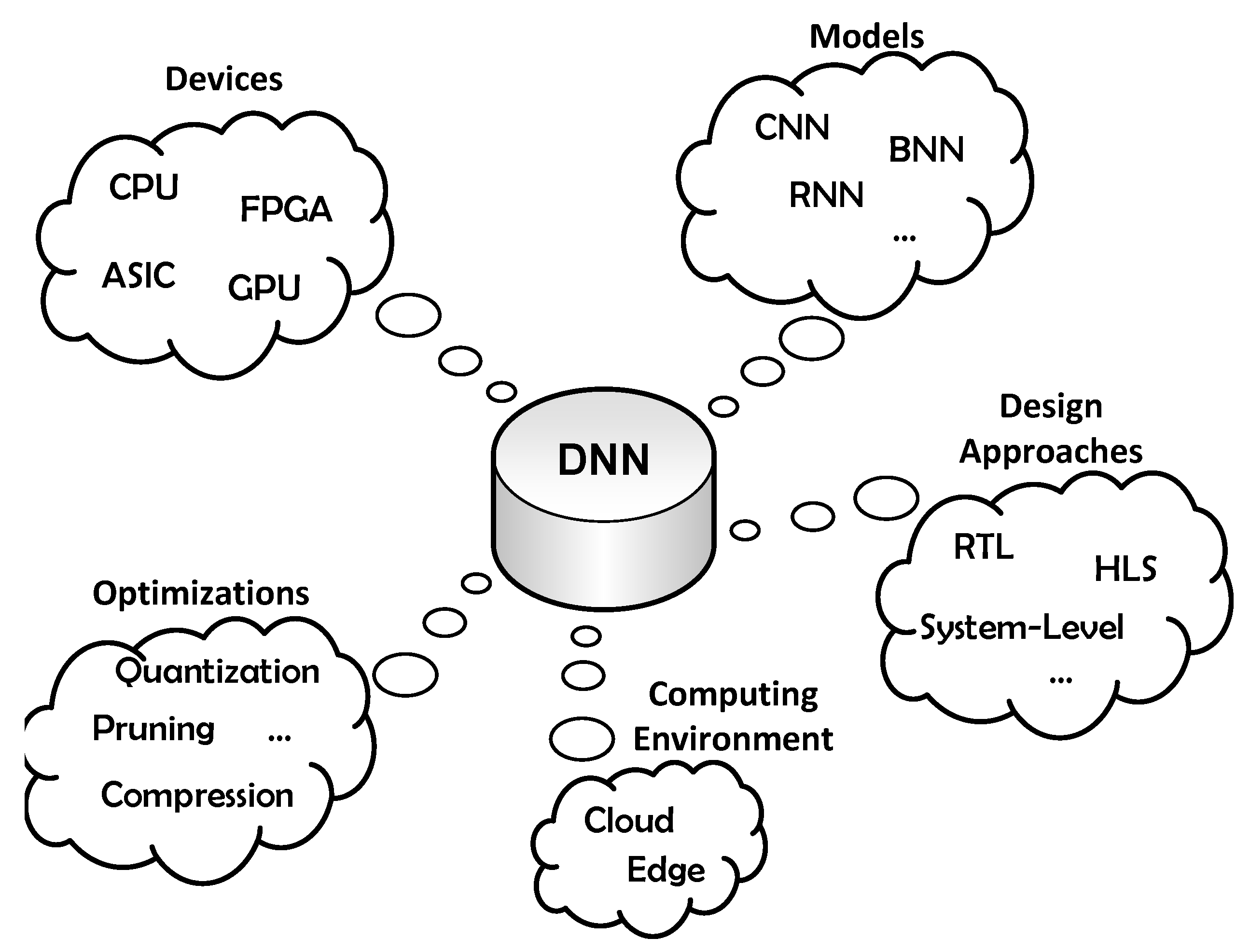
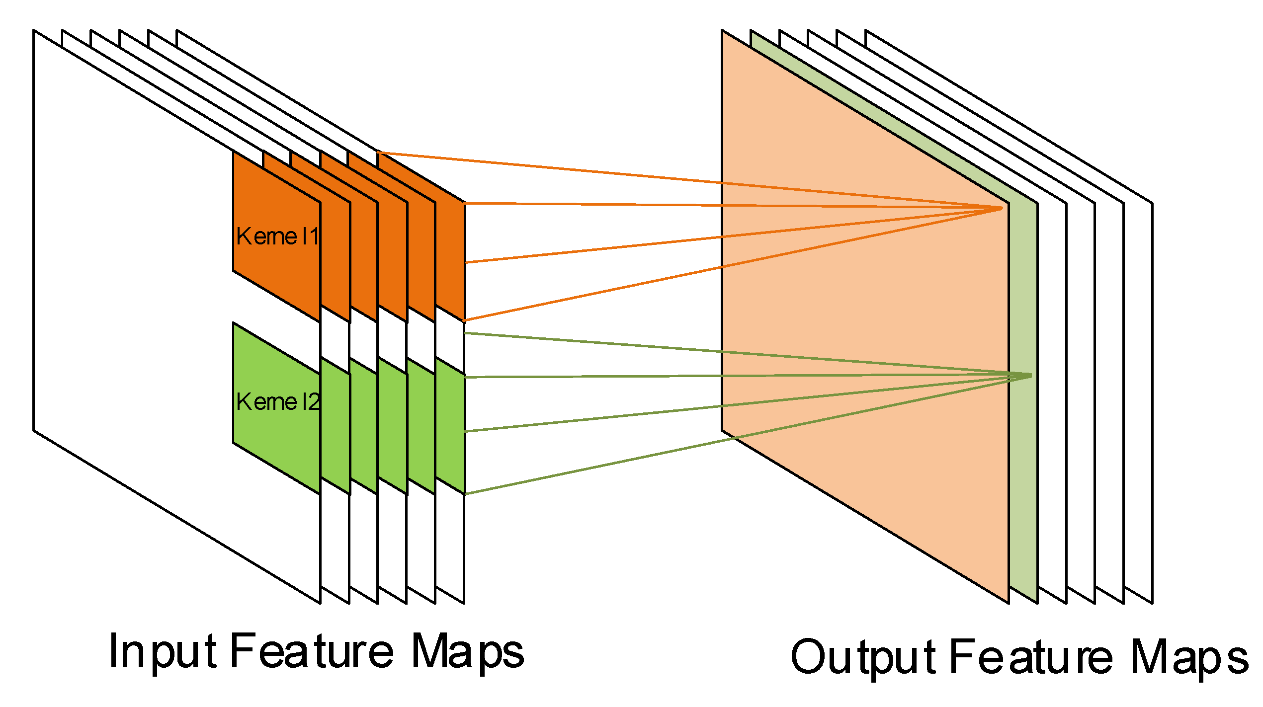
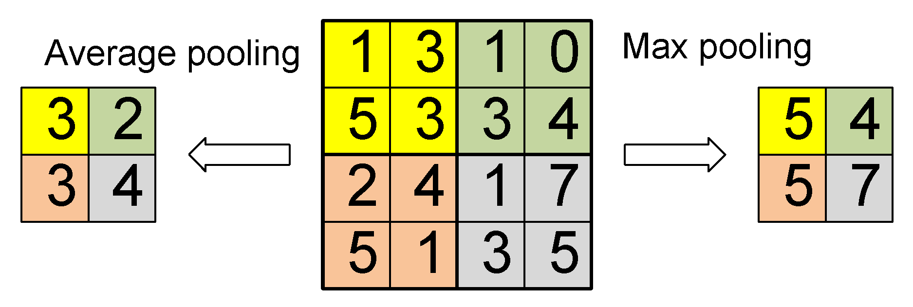
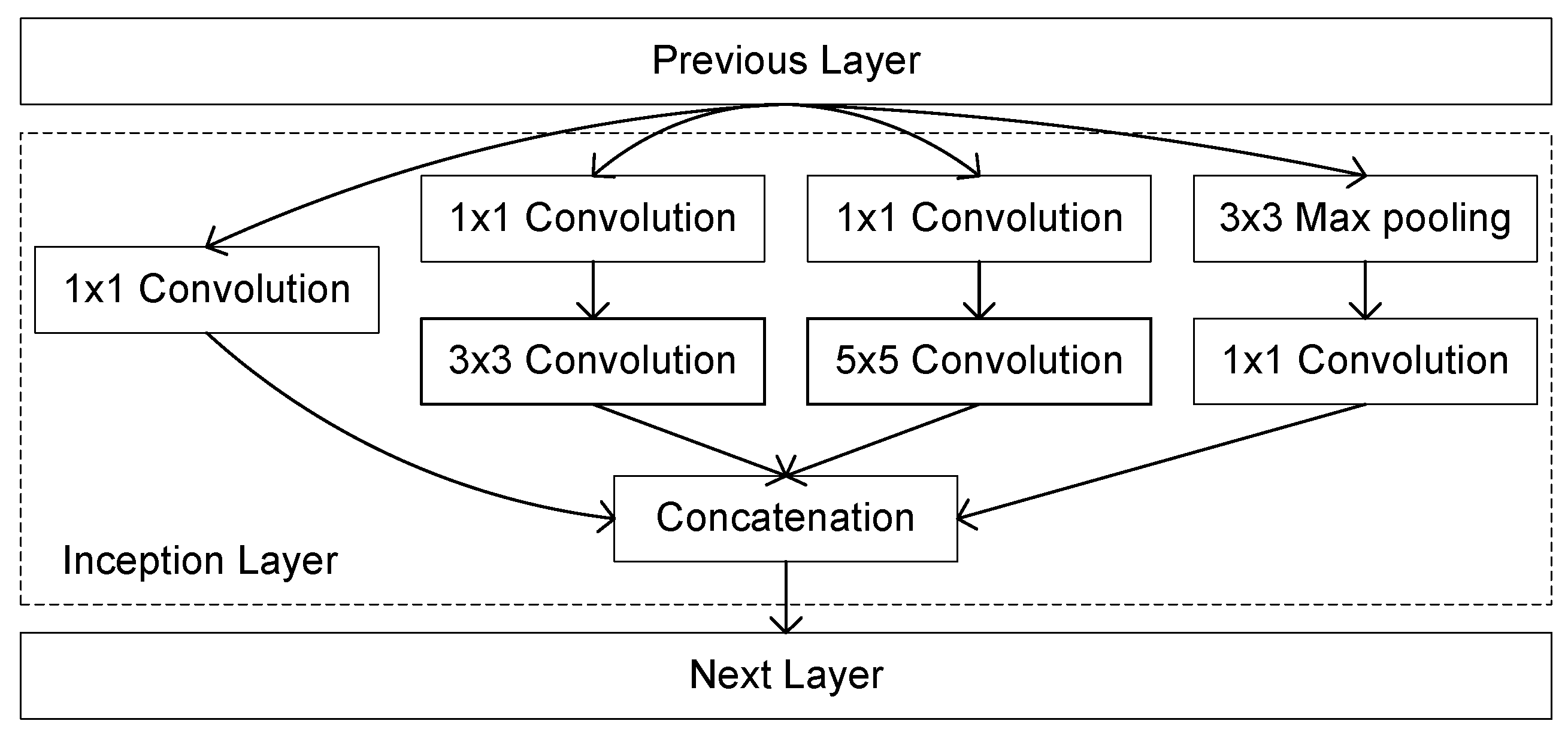
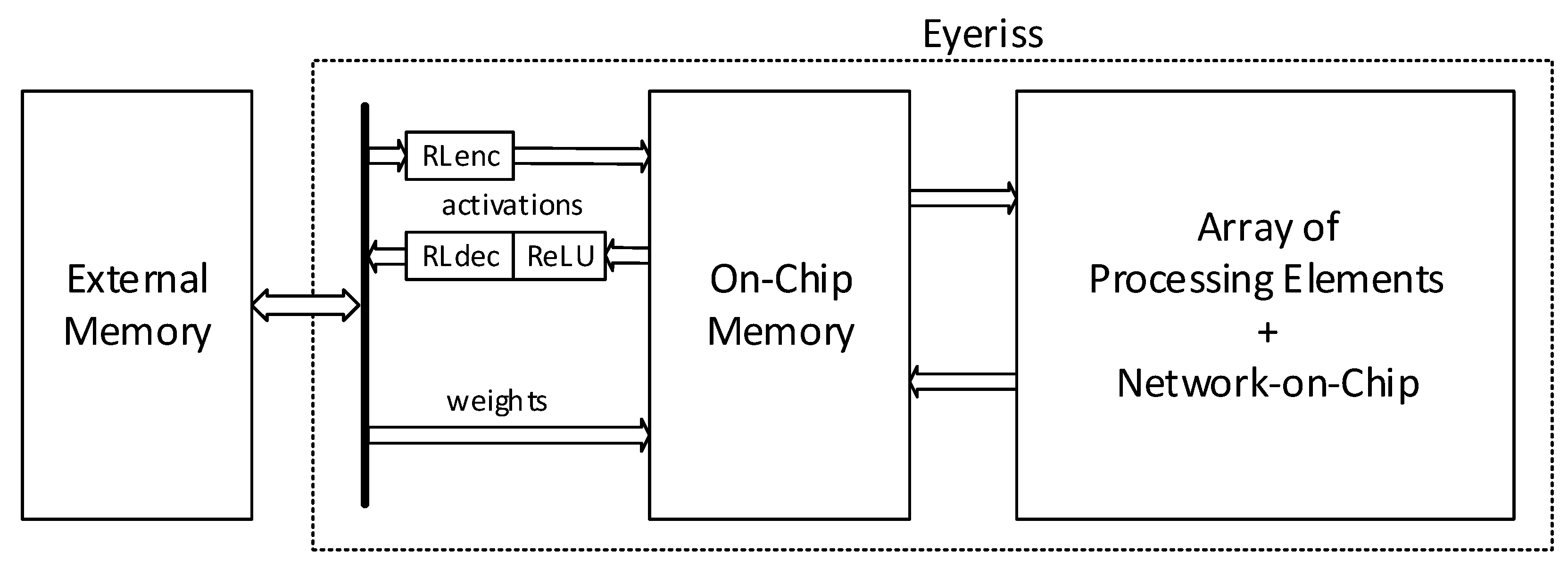
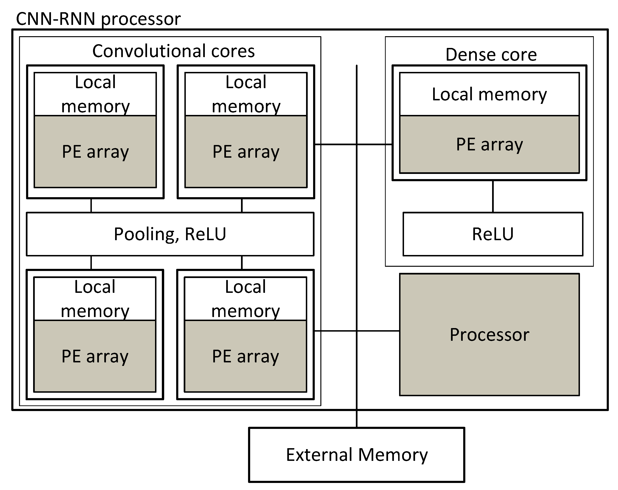
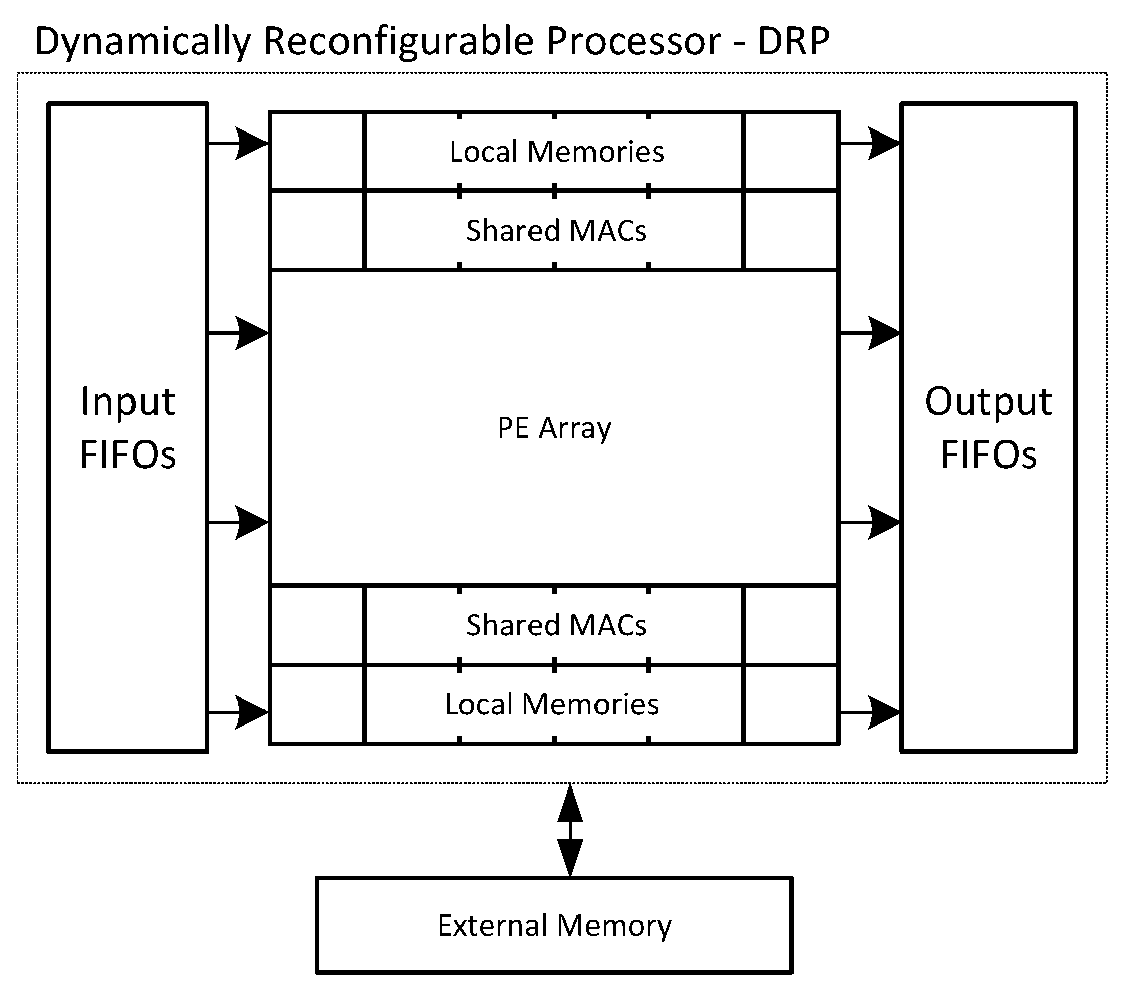
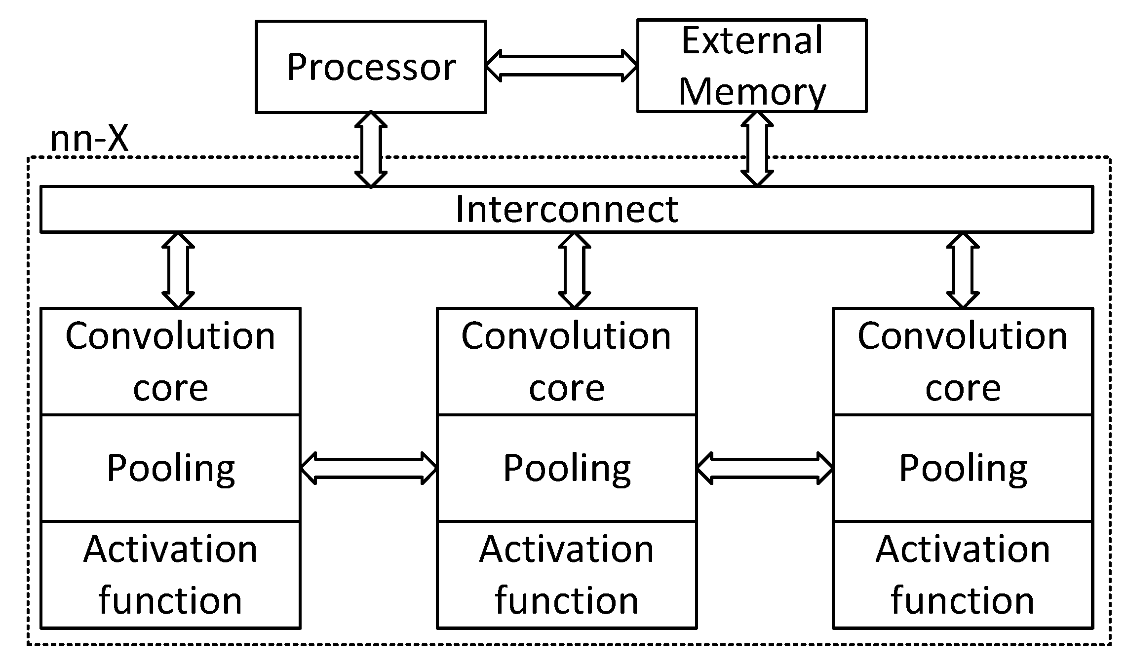
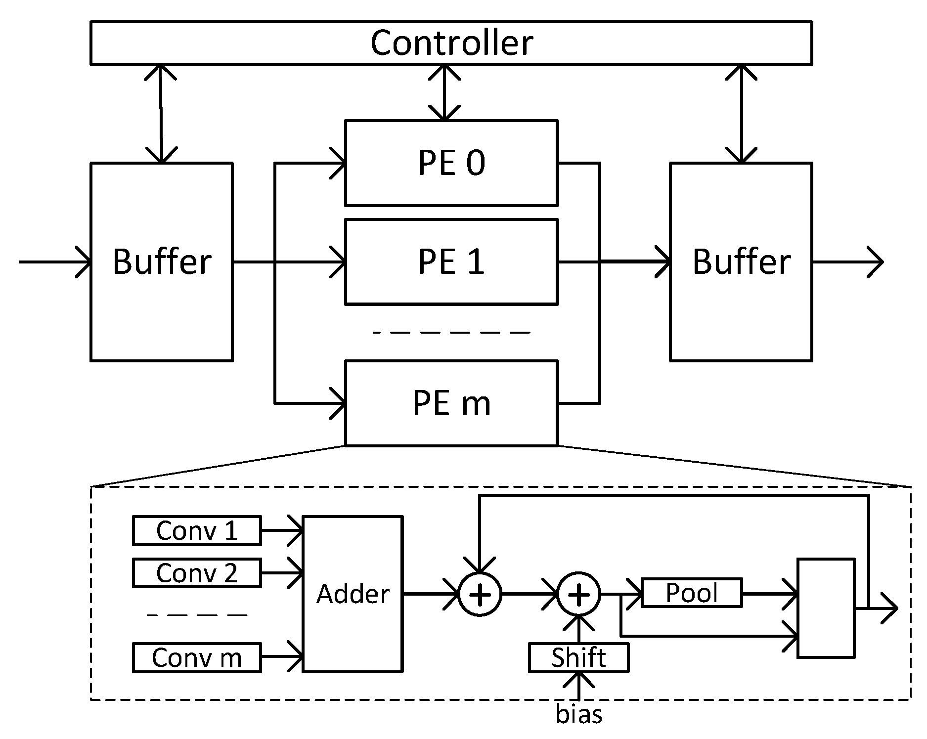
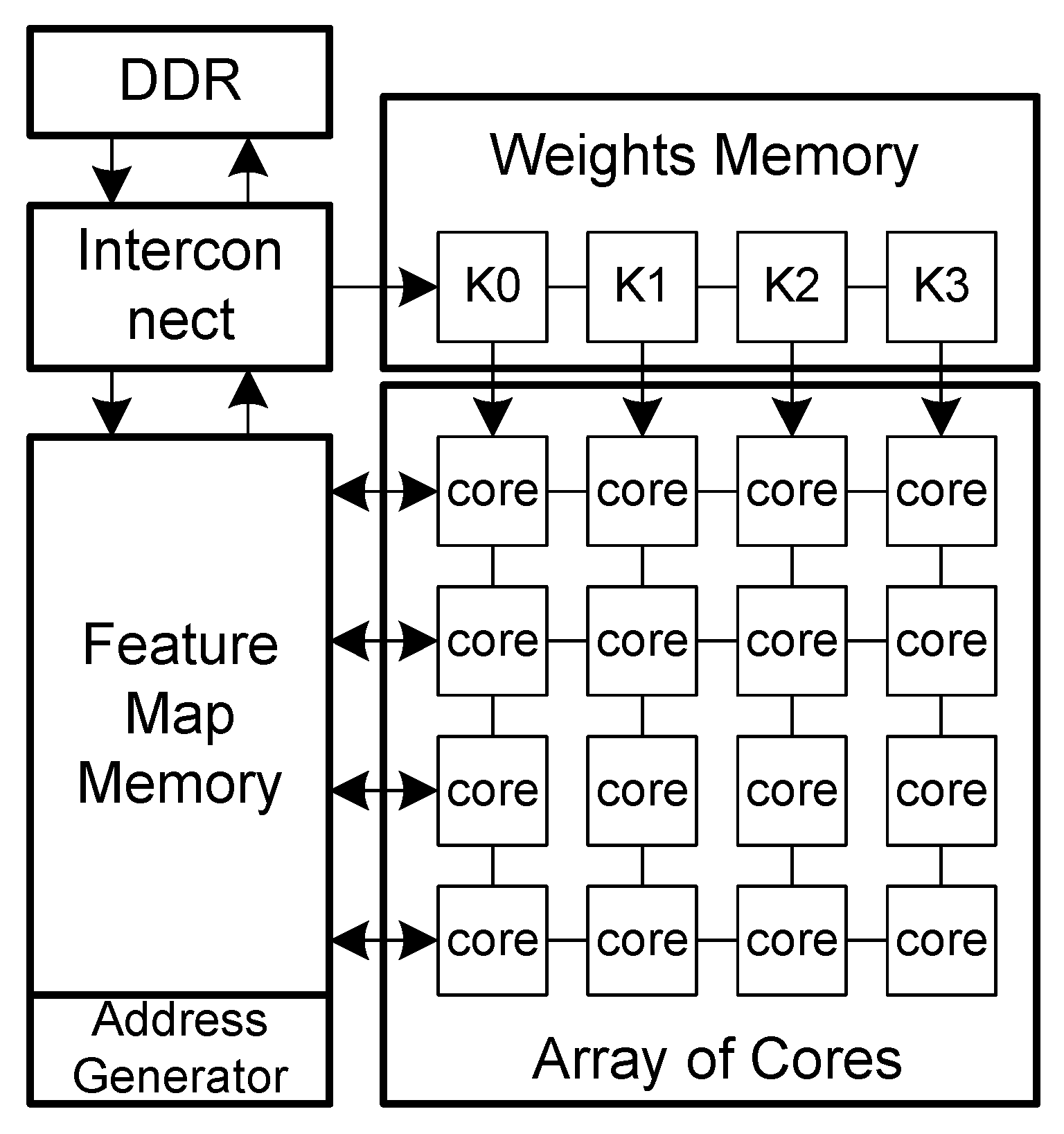
Table 1.
Edge computing versus cloud computing.
| Edge Computing | Cloud Computing |
|---|---|
| Low latency | High latency |
| Time-sensitive response | Not time-sensitive response |
| Low connectivity dependence | High connectivity dependence |
| Task specific processing | Application specific processing |
| Low cost | High cost |
| Difficult to manage (distributed) | Easier to manage (central) |
| Difficult to debug (remote) | Easier to debug (local) |
| Low computing power | High computing power |
| Energy constrained | Not energy constrained |
Table 2.
Complexity and accuracy of known convolutional neural network (CNN) networks.
| Model | # Layers | # Parameters | # MACCs | Error-5(%) |
|---|---|---|---|---|
| AlexNet | 8 | 60 | 650 | 19.7 |
| ZefNet | 8 | 60 | 650 | 11.2 |
| VGG16 | 16 | 138 | 7800 | 10.4 |
| SqueezeNet [24] | 18 | 1.2 | 860 | 19.7 |
| GoogleNet | 22 | 5 | 750 | 6.7 |
| Inception-v3 | 48 | 23.6 | 5700 | 5.6 |
| Inception-v4 | 70 | 35 | 6250 | 5 |
| ResNet-101 | 101 | 40 | 3800 | 6.8 |
| ResNet-152 | 152 | 55 | 5650 | 6.7 |
| ResNet-200 | 200 | 65 | 6850 | 5.8 |
| ResNeXt [25] | 101 | 68 | 4000 | 5.3 |
| DenseNet-201 | 201 | 16.5 | 1500 | 6.3 |
| SENet-154 | 154 | 100 | 10,500 | 4.5 |
| MobileNet-v1 | 28 | 4.2 | 569 | 10 |
| MobileNet-v2 | 28 | 3.5 | 300 | 9 |
| ShuffleNet | 11 | 5.3 | 260 | 10 |
Table 3.
Main features of reconfigurable and configurable architectures for deep neural networks on the edge.
Table 3.
Main features of reconfigurable and configurable architectures for deep neural networks on the edge.
| Architecture | Year | Data | Configurability | Measured GOPs | GOPs/Watt |
|---|---|---|---|---|---|
| nn-X [63] | 2014 | 16-bit | Fine | 23.1 | 25 |
| [2] | 2016 | 16-bit | Fine | 137 | 14.2 |
| fpgaConvNet [66] | 2018 | 16-bit | Fine | 0.48 | - |
| MVTU [35] | 2016 | 1-2 bit | Fine | 2465 | 210 |
| DLAU [71] | 2017 | 48-bit | Fine | - | - |
| Angel-Eye [72] | 2018 | 8/16-bit | Fine | 84/137 | 24.1/14.2 |
| Lite-CNN [73] | 2018 | 8-bit | Fine | 133 | 33 |
| Eyeriss [54] | 2018 | 16-bit | Coarse | 46.2 | 166 |
| CNN-RNN [55] | 2017 | 4-bit | Coarse | 1200 | 3900 |
| SMIV [56] | 2018 | 8-it | Coarse | - | - |
| DRP [57] | 2018 | 16-bit | Coarse | 960 | - |
| DNPU [55] | 2017 | 4/16-bit | Limited | 250 (16b) | 4200 |
| Thinker [74] | 2018 | 8/16-bit | Limited | 368 | 1000 (8b) |
| EV6x [75] | 2017 | 8/12-bit | Limited | - | 2000 |
| NeuPro [76] | 2018 | 8/16-bit | Limited | 2000 | - |
| DNA [77] | 2017 | 8/16-bit | Limited | 1000 | - |
© 2019 by the author. Licensee MDPI, Basel, Switzerland. This article is an open access article distributed under the terms and conditions of the Creative Commons Attribution (CC BY) license (http://creativecommons.org/licenses/by/4.0/).
Share and Cite
MDPI and ACS Style
Véstias, M.P. A Survey of Convolutional Neural Networks on Edge with Reconfigurable Computing. Algorithms 2019, 12, 154. https://doi.org/10.3390/a12080154
AMA Style
Véstias MP. A Survey of Convolutional Neural Networks on Edge with Reconfigurable Computing. Algorithms. 2019; 12(8):154. https://doi.org/10.3390/a12080154
Chicago/Turabian StyleVéstias, Mário P. 2019. "A Survey of Convolutional Neural Networks on Edge with Reconfigurable Computing" Algorithms 12, no. 8: 154. https://doi.org/10.3390/a12080154
Note that from the first issue of 2016, this journal uses article numbers instead of page numbers. See further details here.