Impacts of Atmospheric Pressure on the Annual Maximum of Monthly Sea-Levels in the Northeast Asian Marginal Seas

 , , , ,
Abstract
:1. Introduction
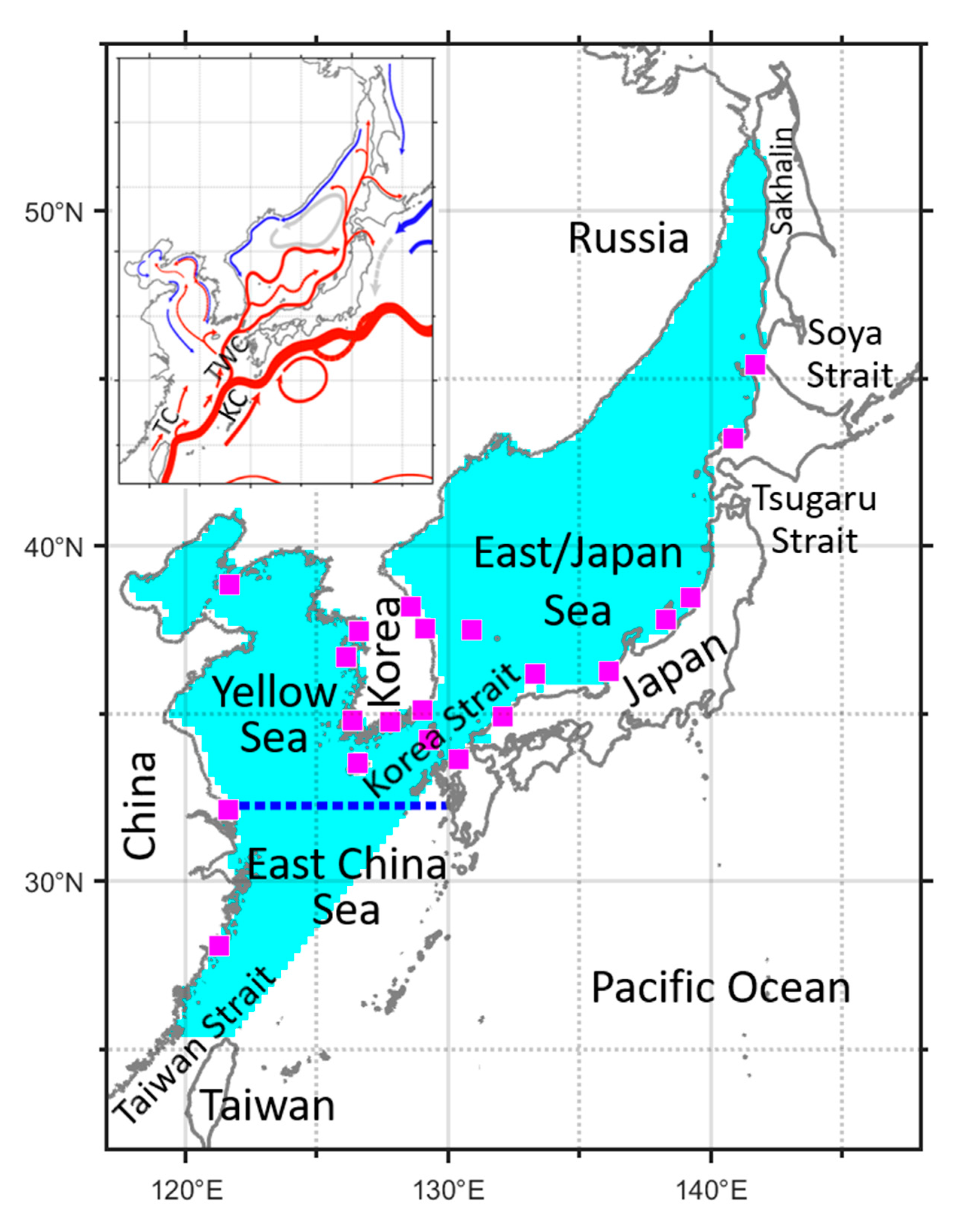
2. Data and Methods
3. Results
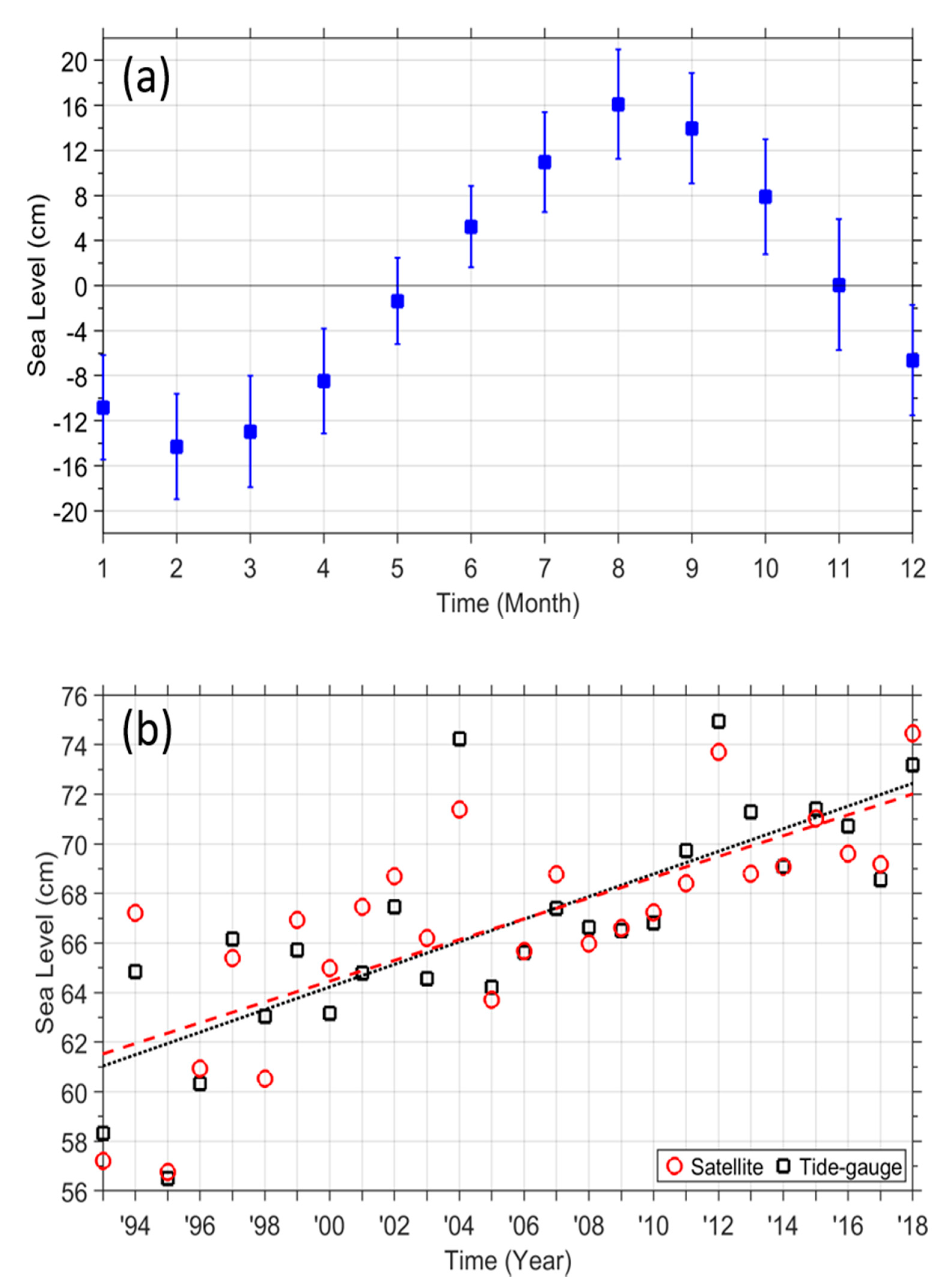
3.1. Long-Term Trend of Sea-Levels in August
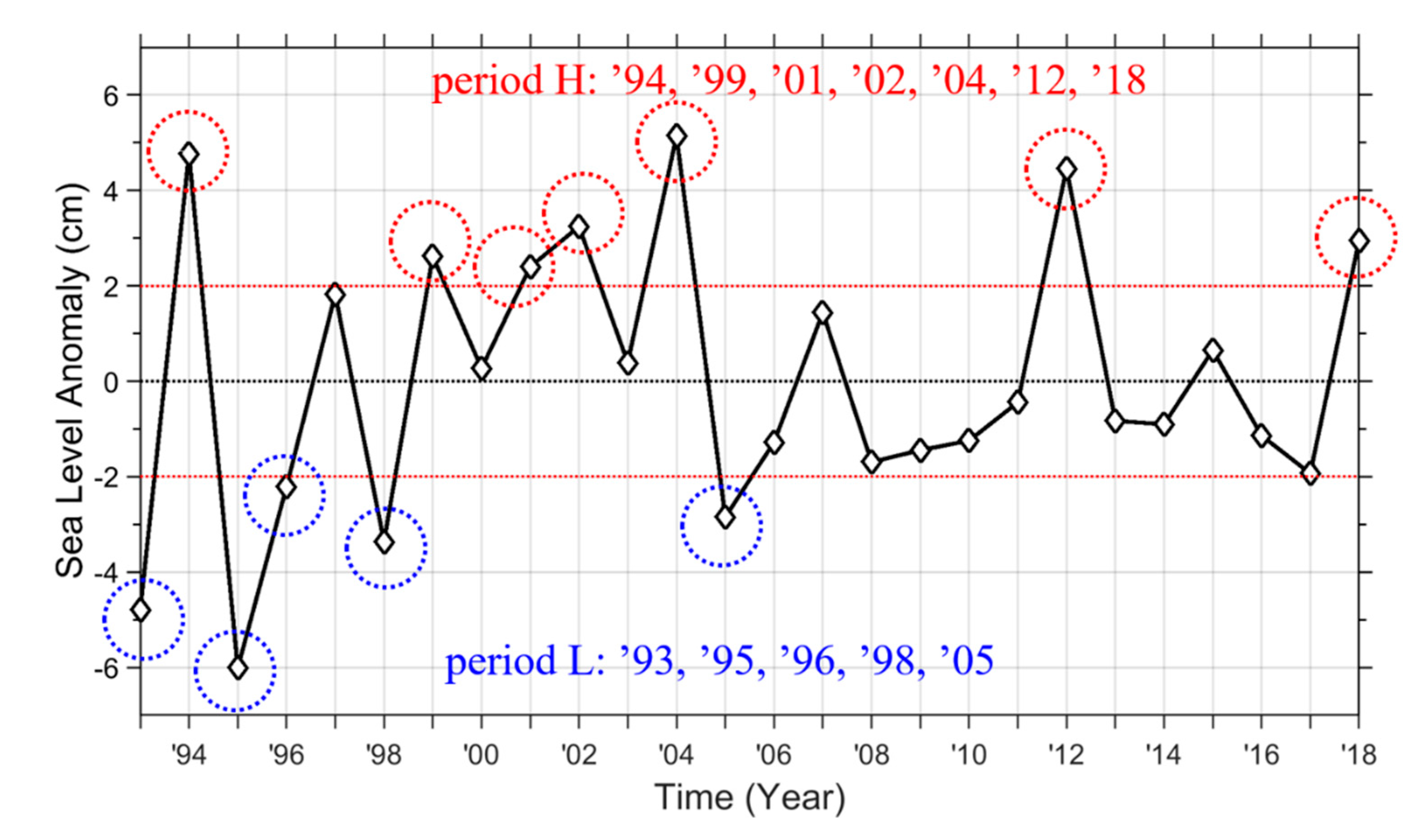
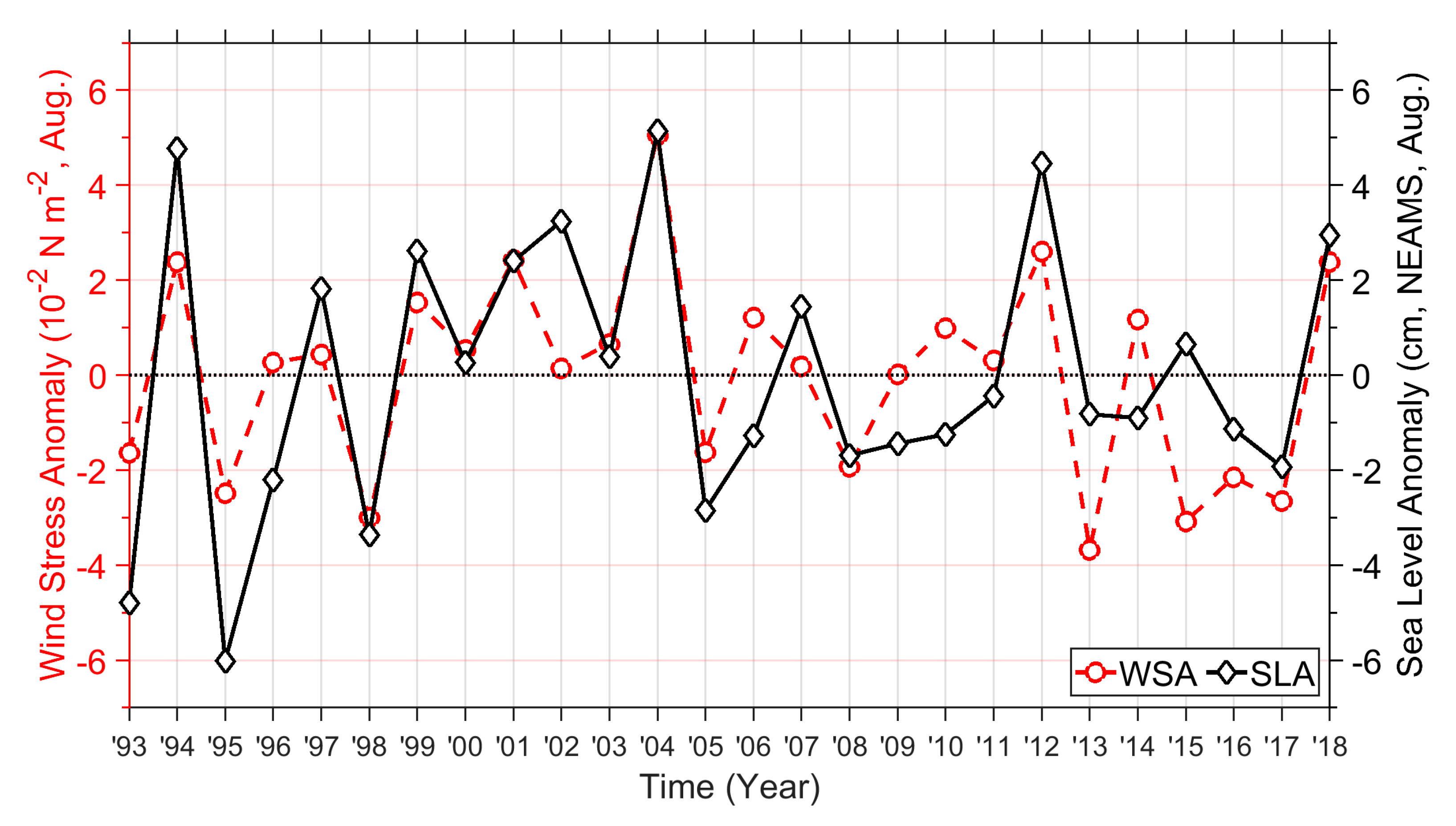
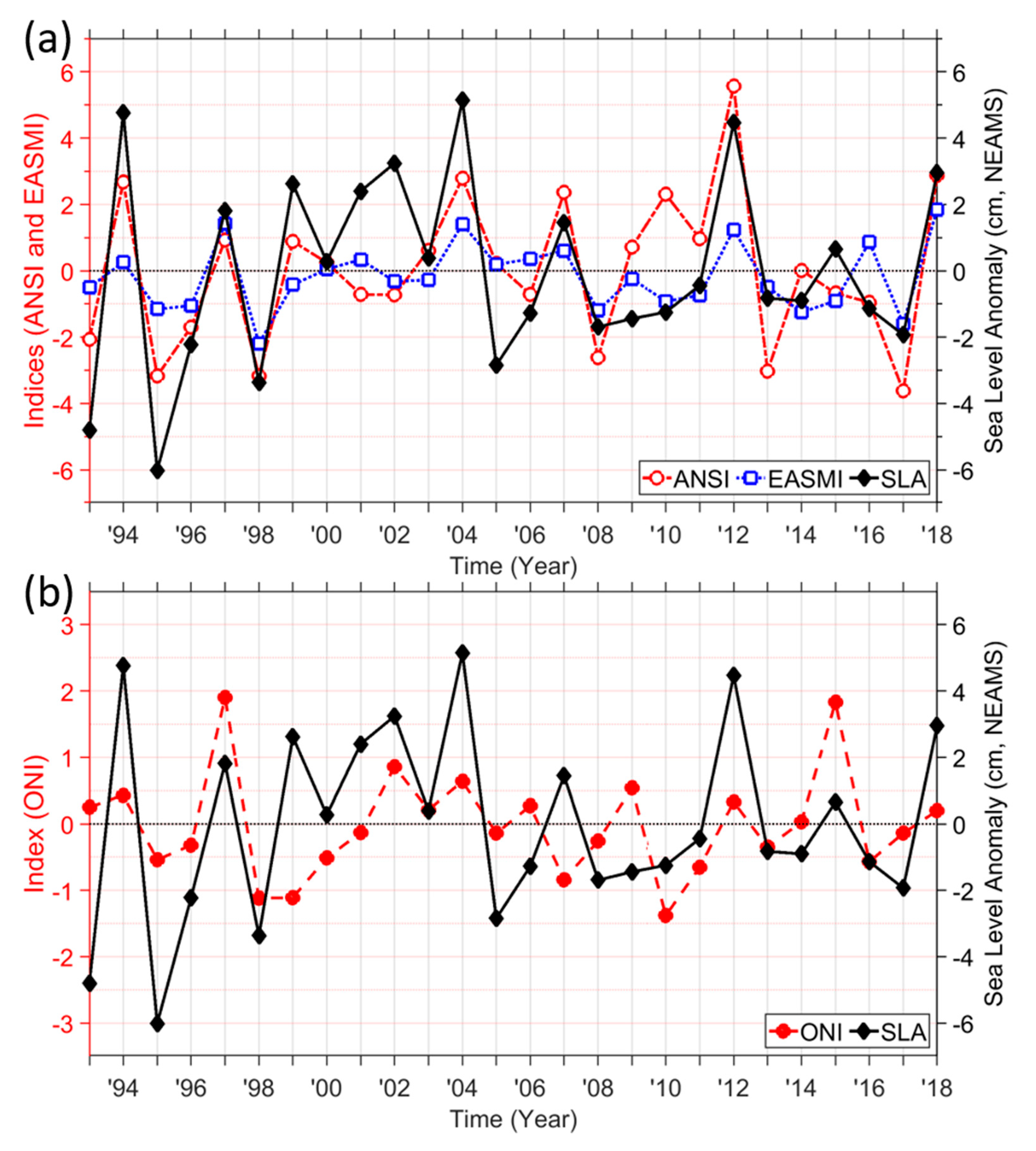
3.2. Interannual Variation of Sea-Level Anomalies in August
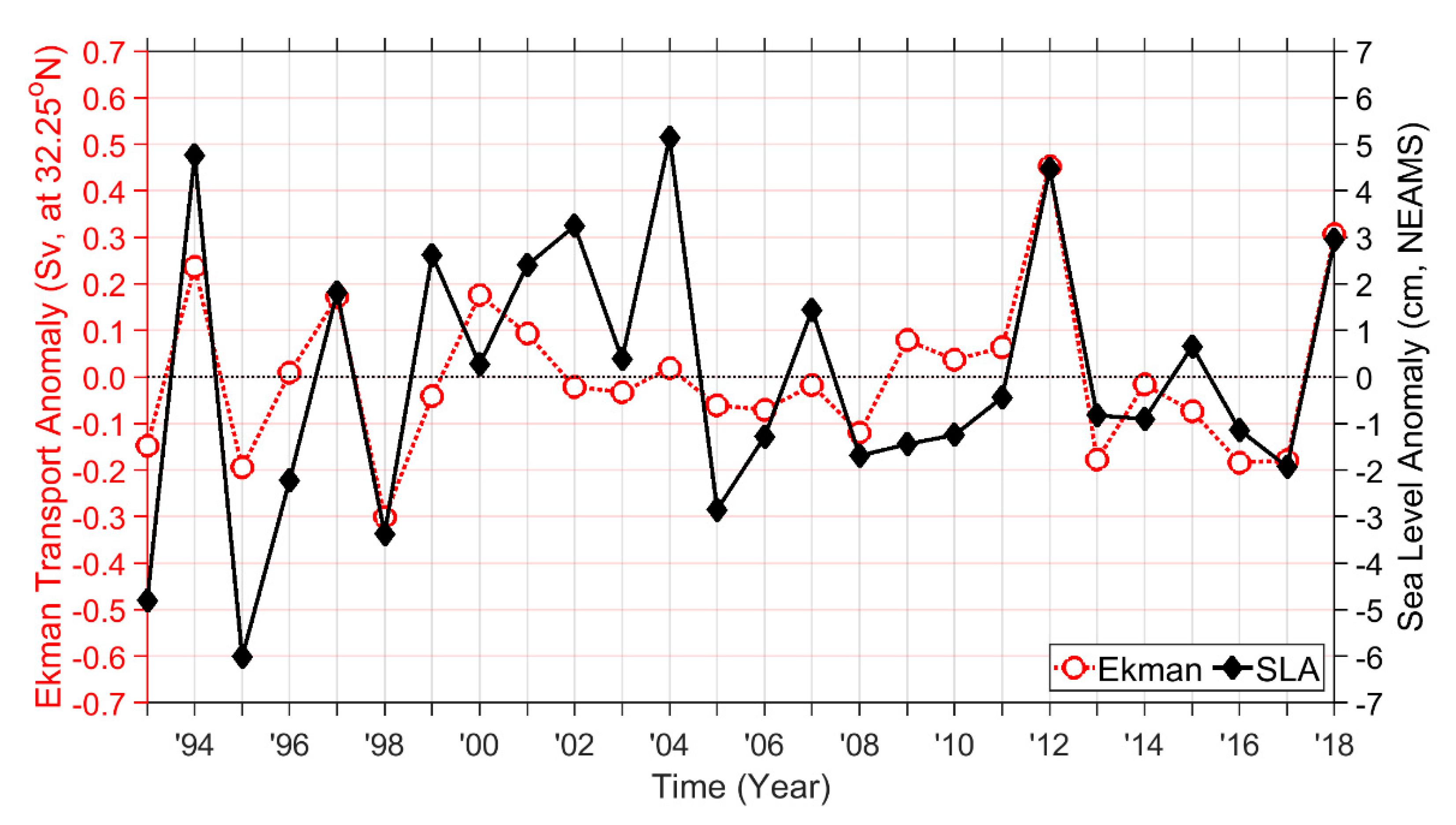
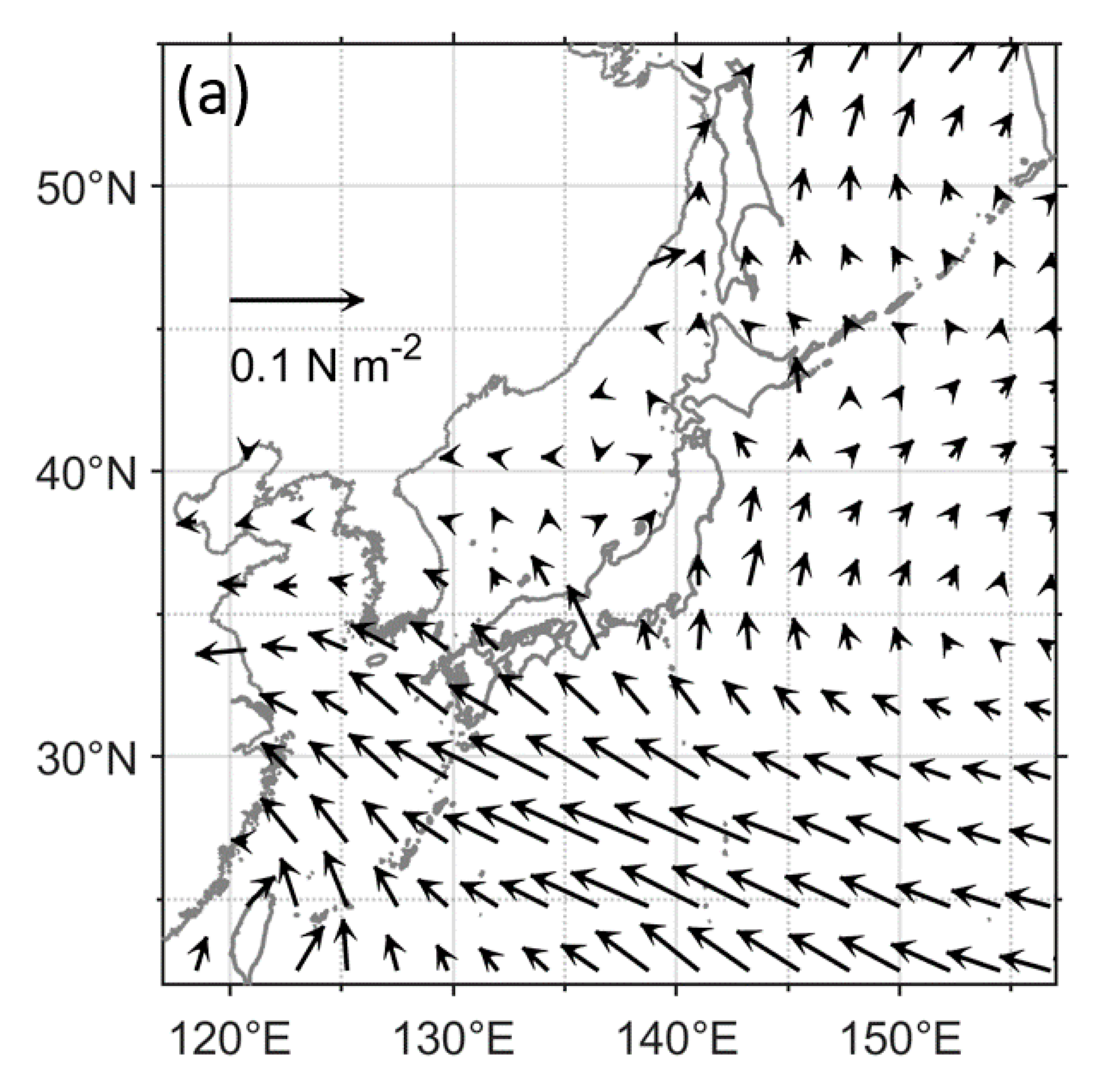
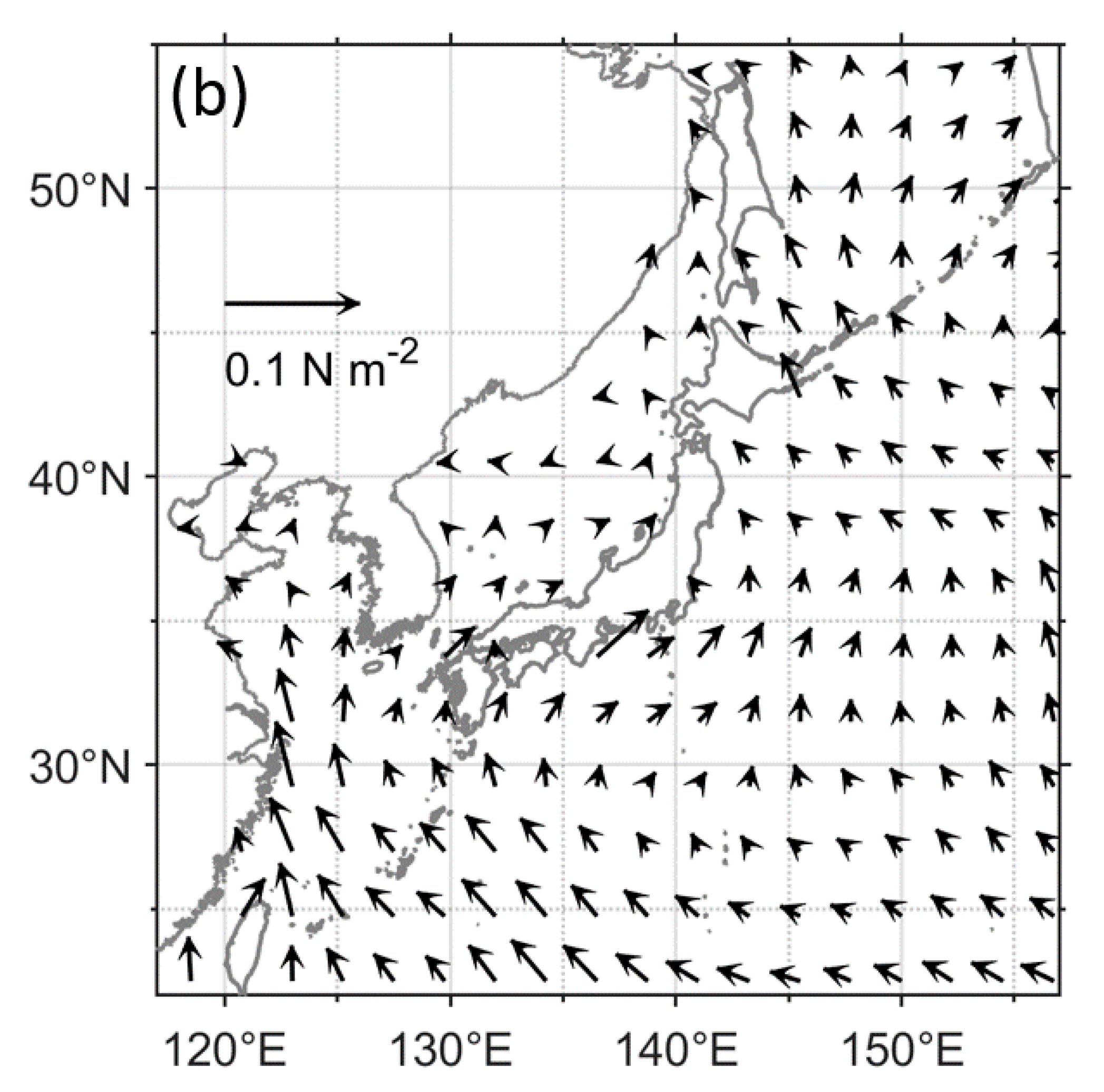
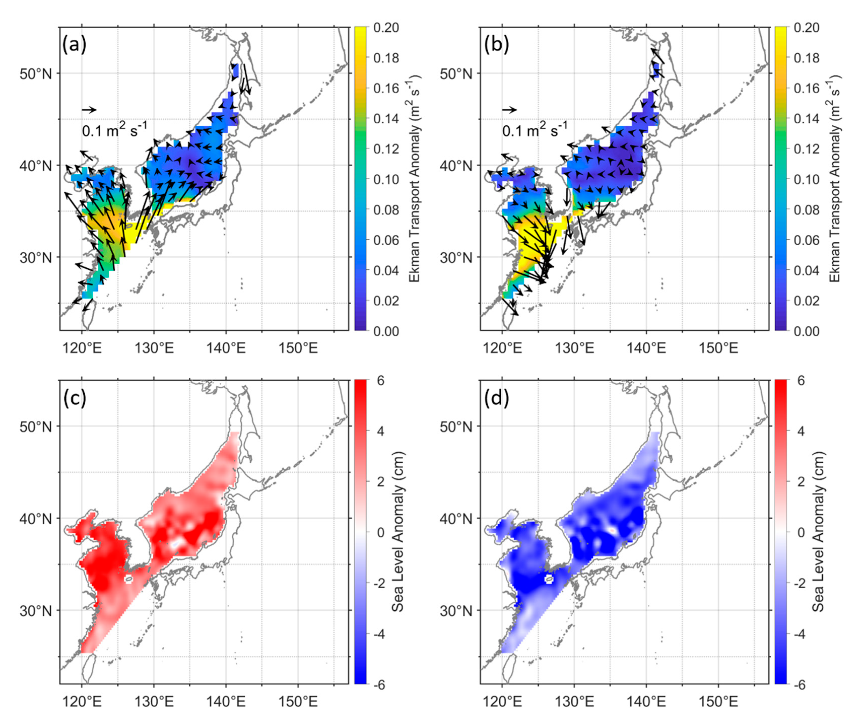
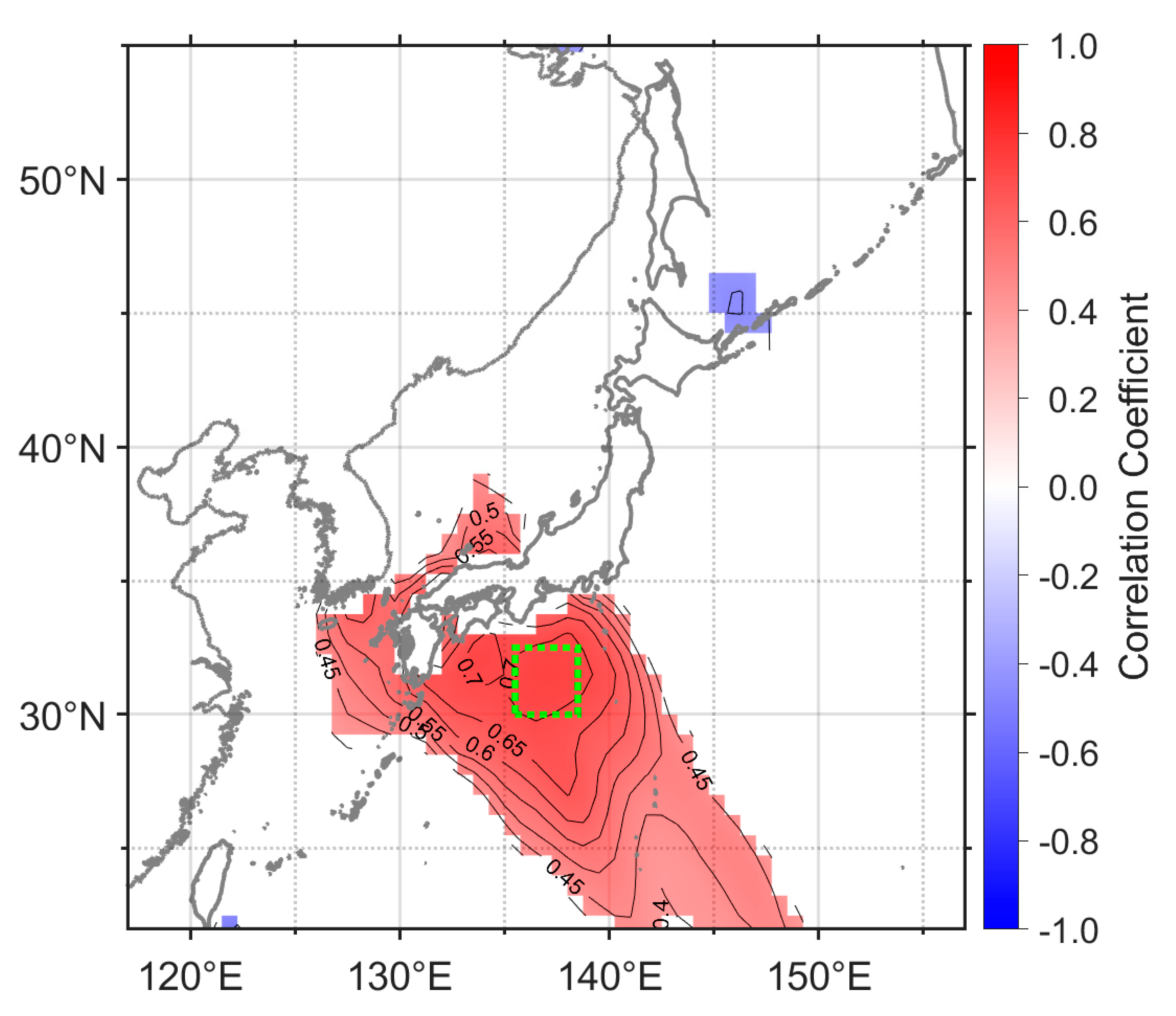
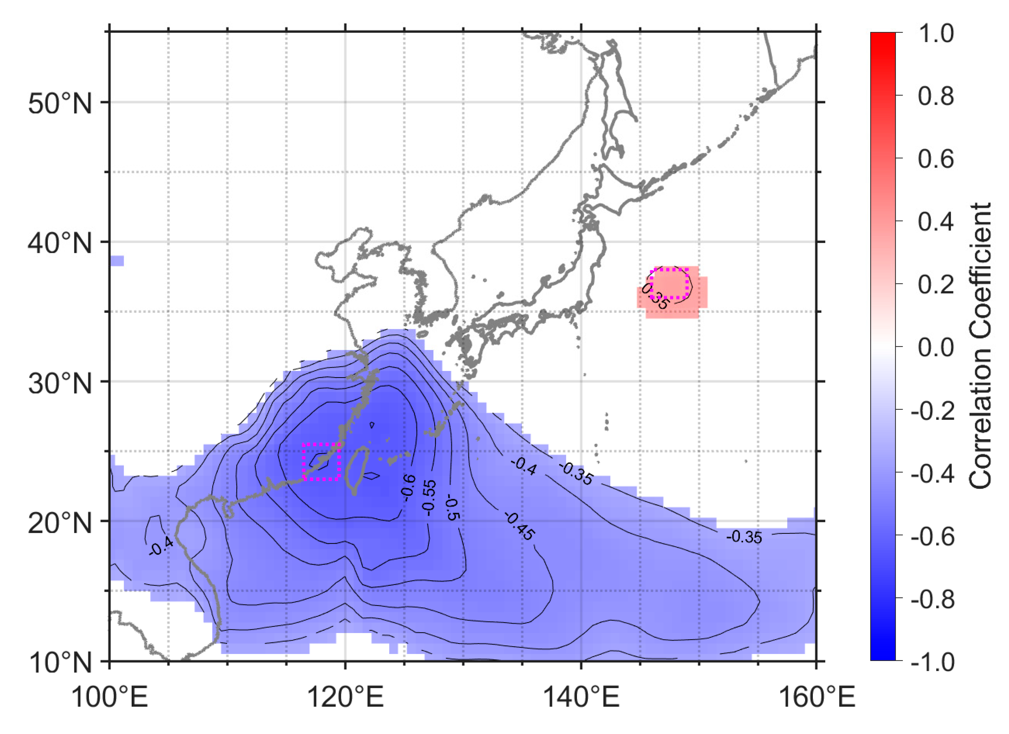
3.3. Ekman Transport and Sea-Level Anomaly
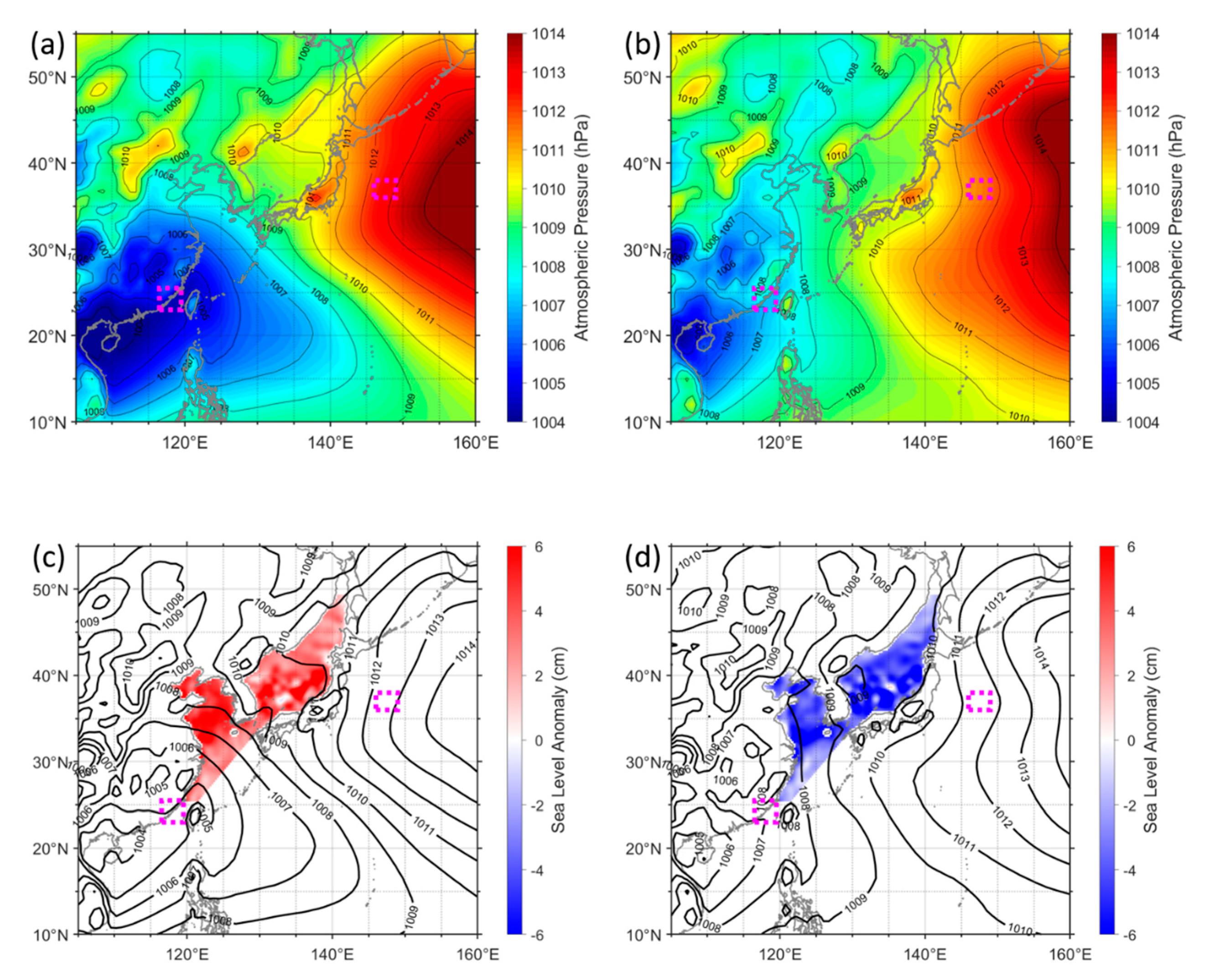
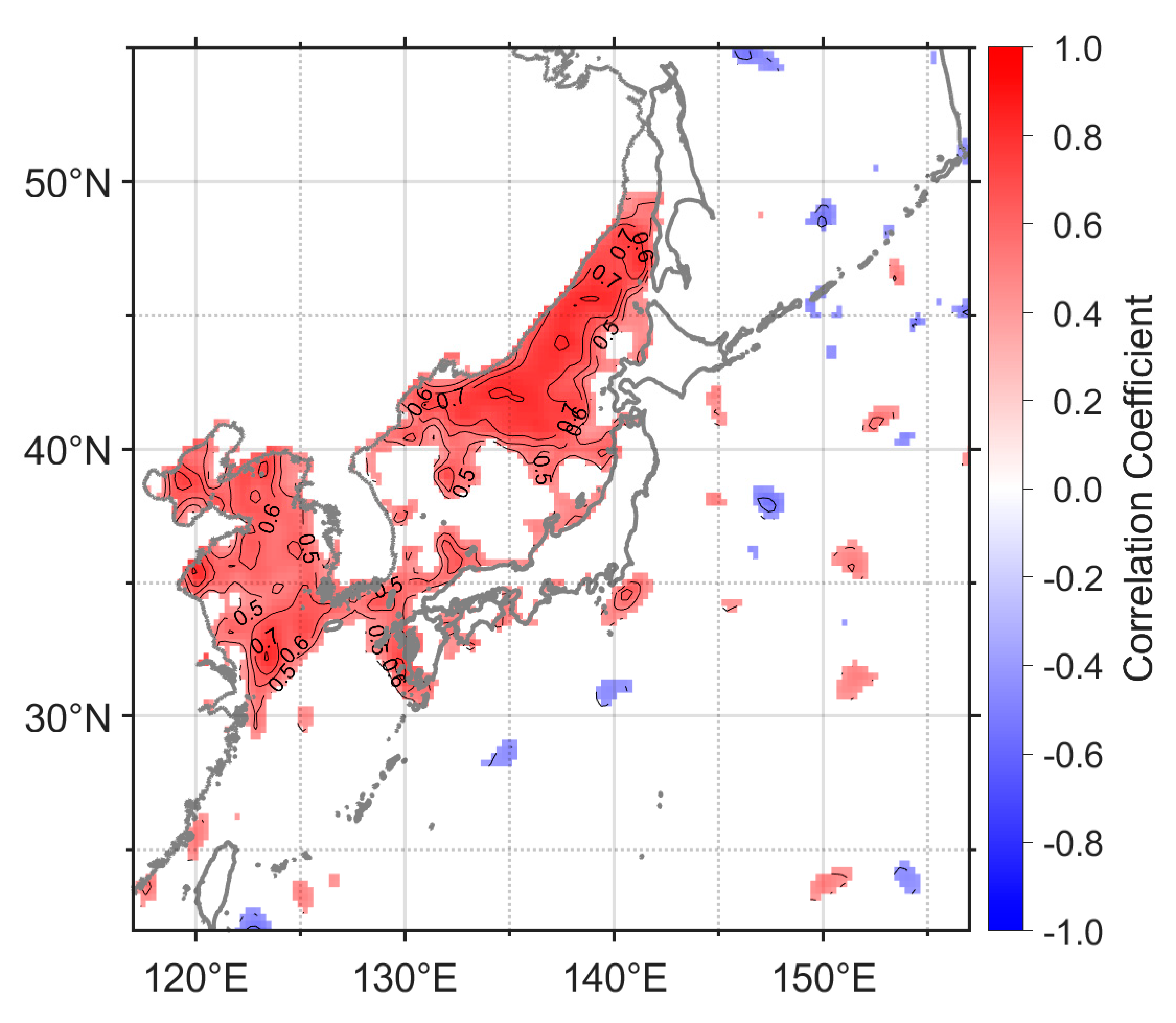
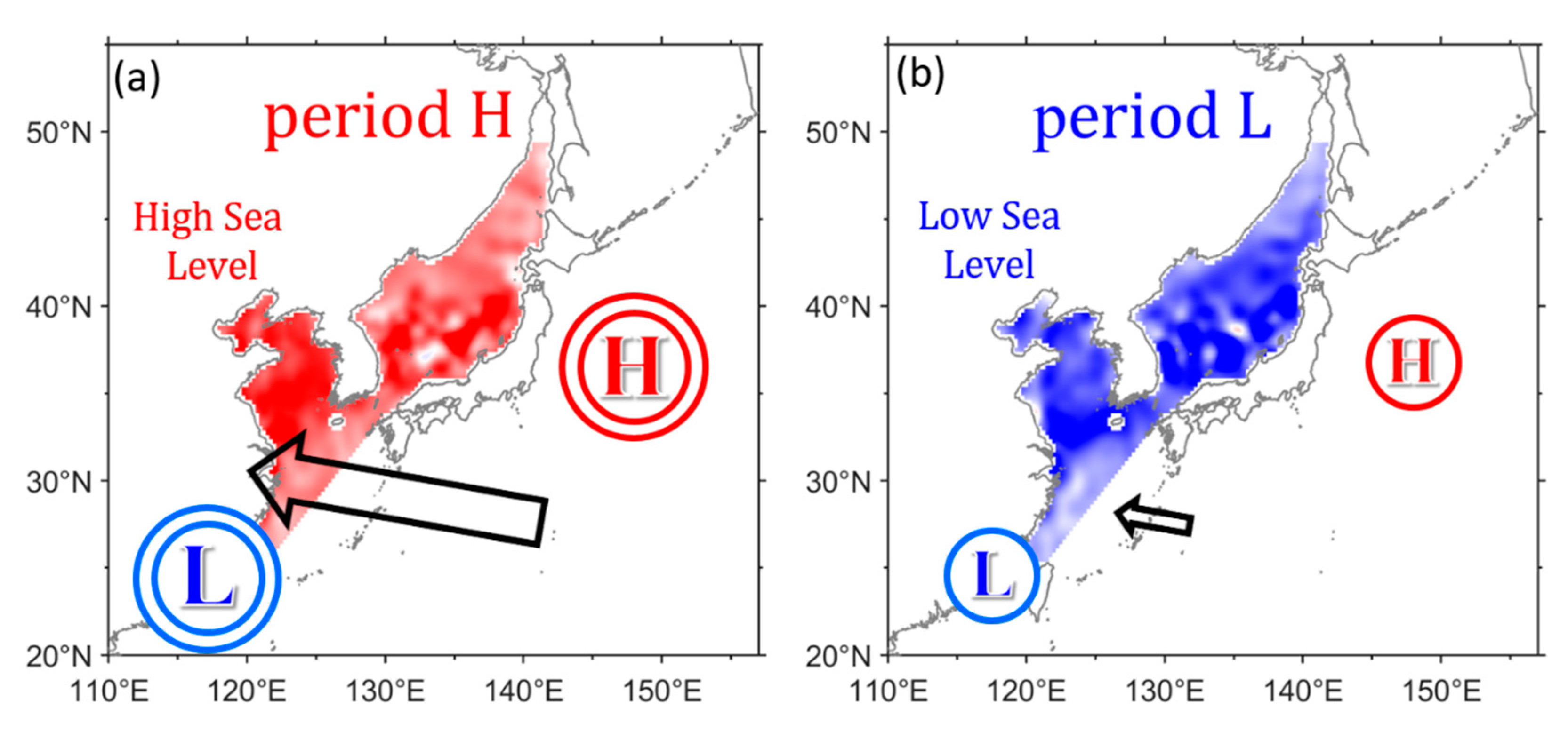
3.4. Atmospheric Pressure Distribution
4. Discussion
5. Conclusions
Author Contributions
Funding
Acknowledgments
Conflicts of Interest
References
- Scheffran, J.; Battaglini, A. Climate and conflicts: The security risks of global warming. Reg. Environ. Chang. 2011, 11, 27–39. [Google Scholar] [CrossRef]
- Gill, A.; Niller, P. The theory of the seasonal variability in the ocean. Deep Sea Res. Oceanogr. Abstr. 1973, 20, 141–177. [Google Scholar] [CrossRef]
- Alley, R.B.; Clark, P.U.; Huybrechts, P.; Joughin, I. Ice-sheet and sea-level changes. Science 2005, 310, 456–460. [Google Scholar] [CrossRef] [PubMed] [Green Version]
- Meehl, G.A.; Washington, W.M.; Collins, W.D.; Arblaster, J.M.; Hu, A.; Buja, L.E.; Strand, W.G.; Teng, H. How much more global warming and sea level rise? Science 2005, 307, 1769–1772. [Google Scholar] [CrossRef] [PubMed] [Green Version]
- Lyu, S.J.; Kim, K.; Perkins, H.T. Atmospheric pressure-forced subinertial variations in the transport through the Korea Strait. Geophys. Res. Lett. 2002, 29, 8-1–8-4. [Google Scholar] [CrossRef]
- Nam, S.H.; Lyu, S.J.; Kim, Y.H.; Kim, K.; Park, J.H.; Watts, D.R. Correction of TOPEX/POSEIDON altimeter data for nonisostatic sea level response to atmospheric pressure in the Japan/East Sea. Geophys. Res. Lett. 2004, 31. [Google Scholar] [CrossRef] [Green Version]
- Lyu, S.J.; Kim, K. Subinertial to interannual transport variations in the Korea Strait and their possible mechanisms. J. Geophys. Res. Ocean. 2005, 110. [Google Scholar] [CrossRef]
- Zuo, J.-C.; He, Q.-Q.; Chen, C.-L.; Chen, M.-X.; Xu, Q. Sea level variability in East China Sea and its response to ENSO. Water Sci. Eng. 2012, 5, 164–174. [Google Scholar] [CrossRef]
- Zhang, S.; Du, L.; Wang, H.; Jiang, H. Regional sea level variation on interannual timescale in the East China Sea. Int. J. Geosci. 2014, 5, 1405. [Google Scholar] [CrossRef] [Green Version]
- Yu, K.; Liu, H.; Chen, Y.; Dong, C.; Dong, J.; Yan, Y.; Wang, D. Impacts of the mid-latitude westerlies anomaly on the decadal sea level variability east of China. Clim. Dyn. 2019, 53, 5985–5998. [Google Scholar] [CrossRef]
- Choi, B.-J.; Haidvogel, D.B.; Cho, Y.-K. Interannual variation of the Polar Front in the Japan/East Sea from summertime hydrography and sea level data. J. Mar. Syst. 2009, 78, 351–362. [Google Scholar] [CrossRef]
- Ohshima, K.I.; Simizu, D.; Ebuchi, N.; Morishima, S.; Kashiwase, H. Volume, heat, and salt transports through the Soya Strait and their seasonal and interannual variations. J. Phys. Oceanogr. 2017, 47, 999–1019. [Google Scholar] [CrossRef]
- Amiruddin, A.; Haigh, I.; Tsimplis, M.; Calafat, F.; Dangendorf, S. The seasonal cycle and variability of sea level in the South China S ea. J. Geophys. Res. Ocean. 2015, 120, 5490–5513. [Google Scholar] [CrossRef] [Green Version]
- Noone, K.J.; Sumaila, U.R.; Diaz, R.J. Managing Ocean Environments in a Changing Climate: Sustainability and Economic Perspectives; Elsevier: Amsterdam, The Netherlands, 2013. [Google Scholar]
- Marcos, M.; Tsimplis, M.N.; Calafat, F.M. Inter-annual and decadal sea level variations in the north-western Pacific marginal seas. Prog. Oceanogr. 2012, 105, 4–21. [Google Scholar] [CrossRef]
- Rio, M.; Guinehut, S.; Larnicol, G. New CNES-CLS09 global mean dynamic topography computed from the combination of GRACE data, altimetry, and in situ measurements. J. Geophys. Res. Ocean. 2011, 116. [Google Scholar] [CrossRef]
- AVISO. MDT; CNES-CLS18. 2020. Available online: https://www.aviso.altimetry.fr/en/data/products/auxiliary-products/mdt.html (accessed on 4 March 2020).
- Taburet, G.; Pujol, M.-I. Sea Level TAC-DUACS Products. 2020. Available online: https://resources.marine.copernicus.eu/documents/QUID/CMEMS-SL-QUID-008-032-062.pdf (accessed on 30 March 2020).
- Sealevel_GLO_PHY_L4_REP_Observations_008_047. Available online: Ftp://my.cmems-du.eu/Core/SEALEVEL_GLO_PHY_L4_REP_OBSERVATIONS_008_047 (accessed on 4 March 2020).
- CMEMS. Global Ocean Gridded L4 Sea Surface Heights and Derived Variables Reprocessed (1993-Ongoing). 2020. Available online: http://marine.copernicus.eu/services-portfolio/access-to-products/?option=com_csw&view=details&product_id=SEALEVEL_GLO_PHY_L4_REP_OBSERVATIONS_008_047 (accessed on 4 March 2020).
- Holgate, S.J.; Matthews, A.; Woodworth, P.L.; Rickards, L.J.; Tamisiea, M.E.; Bradshaw, E.; Foden, P.R.; Gordon, K.M.; Jevrejeva, S.; Pugh, J. New data systems and products at the permanent service for mean sea level. J. Coast. Res. 2013, 29, 493–504. [Google Scholar] [CrossRef]
- PSMSL. Tide Gauge Data. 2020. Available online: http://www.psmsl.org/data/obtaining/ (accessed on 20 January 2020).
- Mathers, E.; Woodworth, P. Departures from the local inverse barometer model observed in altimeter and tide gauge data and in a global barotropic numerical model. J. Geophys. Res. Ocean. 2001, 106, 6957–6972. [Google Scholar] [CrossRef]
- Wunsch, C.; Stammer, D. Atmospheric loading and the oceanic “inverted barometer” effect. Rev. Geophys. 1997, 35, 79–107. [Google Scholar] [CrossRef]
- Cheney, R.; Miller, L.; Agreen, R.; Doyle, N.; Lillibridge, J. Topex/poseidon: The 2-cm solution. J. Geophys. Res. Ocean. 1994, 99, 24555–24563. [Google Scholar] [CrossRef]
- Isobe, A. The taiwan-tsushima warm current system: Its path and the transformation of the water mass in the East China Sea. J. Oceanogr. 1999, 55, 185–195. [Google Scholar] [CrossRef]
- Liu, X.; Liu, Y.; Guo, L.; Rong, Z.; Gu, Y.; Liu, Y. Interannual changes of sea level in the two regions of East China Sea and different responses to ENSO. Glob. Planet. Chang. 2010, 72, 215–226. [Google Scholar] [CrossRef]
- Li, Y.; Zuo, J.; Lu, Q.; Zhang, H.; Chen, M. Impacts of wind forcing on sea level variations in the East China Sea: Local and remote effects. J. Mar. Syst. 2016, 154, 172–180. [Google Scholar] [CrossRef]
- Surry, A.; King, J.R. A New Method for Calculating ALPI: The Aleutian Low Pressure Index; Fisheries and Oceans Canada, Science Branch, Pacific Region, Pacific Biological Station: Nanaimo, BC, Canada, 2015. [Google Scholar]
- Rigor, I.G.; Wallace, J.M.; Colony, R.L. Response of sea ice to the Arctic Oscillation. J. Clim. 2002, 15, 2648–2663. [Google Scholar] [CrossRef] [Green Version]
- Li, J.; Zeng, Q. A unified monsoon index. Geophys. Res. Lett. 2002, 29, 115-111–115-114. [Google Scholar] [CrossRef]
- Di Lorenzo, E.; Schneider, N.; Cobb, K.M.; Franks, P.; Chhak, K.; Miller, A.J.; McWilliams, J.C.; Bograd, S.J.; Arango, H.; Curchitser, E. North Pacific Gyre Oscillation links ocean climate and ecosystem change. Geophys. Res. Lett. 2008, 35. [Google Scholar] [CrossRef] [Green Version]
- Trenberth, K.E.; Hurrell, J.W. Decadal atmosphere-ocean variations in the Pacific. Clim. Dyn. 1994, 9, 303–319. [Google Scholar] [CrossRef]
- Hafez, Y. Study on the relationship between the oceanic nino index and surface air temperature and precipitation rate over the Kingdom of Saudi Arabia. J. Geosci. Environ. Prot. 2016, 4, 146. [Google Scholar] [CrossRef] [Green Version]
- Wu, B.; Wang, J. Winter Arctic oscillation, Siberian high and East Asian winter monsoon. Geophys. Res. Lett. 2002, 29, 3-1–3-4. [Google Scholar] [CrossRef]


© 2020 by the authors. Licensee MDPI, Basel, Switzerland. This article is an open access article distributed under the terms and conditions of the Creative Commons Attribution (CC BY) license (http://creativecommons.org/licenses/by/4.0/).
Share and Cite
Han, M.; Cho, Y.-K.; Kang, H.-W.; Nam, S.; Byun, D.-S.; Jeong, K.-Y.; Lee, E. Impacts of Atmospheric Pressure on the Annual Maximum of Monthly Sea-Levels in the Northeast Asian Marginal Seas. J. Mar. Sci. Eng. 2020, 8, 425. https://doi.org/10.3390/jmse8060425
Han M, Cho Y-K, Kang H-W, Nam S, Byun D-S, Jeong K-Y, Lee E. Impacts of Atmospheric Pressure on the Annual Maximum of Monthly Sea-Levels in the Northeast Asian Marginal Seas. Journal of Marine Science and Engineering. 2020; 8(6):425. https://doi.org/10.3390/jmse8060425
Chicago/Turabian StyleHan, MyeongHee, Yang-Ki Cho, Hyoun-Woo Kang, SungHyun Nam, Do-Seong Byun, Kwang-Young Jeong, and Eunil Lee. 2020. "Impacts of Atmospheric Pressure on the Annual Maximum of Monthly Sea-Levels in the Northeast Asian Marginal Seas" Journal of Marine Science and Engineering 8, no. 6: 425. https://doi.org/10.3390/jmse8060425