Article

A Numerical Study of Windstorms in the Lee of the Taebaek Mountains, South Korea: Characteristics and Generation Mechanisms

1
School of Earth and Environmental Sciences, Seoul National University, Seoul 08826, Korea
2
Precipitating Convection Group, Max Planck Institute for Meteorology, 20146 Hamburg, Germany
*
Author to whom correspondence should be addressed.
Atmosphere 2020, 11(4), 431; https://doi.org/10.3390/atmos11040431
Submission received: 19 February 2020 / Revised: 16 April 2020 / Accepted: 22 April 2020 / Published: 24 April 2020
(This article belongs to the Special Issue Advancements in Mesoscale Weather Analysis and Prediction)

Abstract

:
The Yeongdong region, located east of the Taebaek Mountains, South Korea, often experiences severe windstorms in spring, causing a lot of damages, especially when forest fires spread out rapidly by strong winds. Here, the characteristics and generation mechanisms of the windstorms in the Yeongdong region on 8 April 2012 are examined through a high-resolution Weather Research and Forecasting (WRF) model simulation. In the Yangyang area, the steep descent of the isentropes on the lee slope of the mountain and their recovery farther leeward are seen. Inversion layers and incoming flow in hydraulic jump regime suggest that the hydraulic jump is responsible for the downslope windstorm. In the Jangjeon area, the plume-shaped wind pattern extending seaward from the gap exit is seen when the sea-level pressure difference between the gap inside and the gap exit, being responsible for the gap winds, is large. In the Uljin area, downslope windstorms pass over the region with weak wind, low Richardson number, and deep planetary boundary layer (PBL), making banded pattern in the wind and PBL height fields. This study demonstrates that the characteristics of the windstorms in the lee of the Taebaek Mountains and their generation mechanisms differ depending on local topographic features.

1. Introduction

There are many meteorological phenomena directly associated with topography, which include mountain/valley winds, downslope windstorms, gap winds, lee waves, lee vortices, cold-air damming, and banner clouds [1]. When winds blow down on the lee slope of a mountain, they become strong, occasionally producing severe downslope windstorms. Downslope windstorms are observed in many regions of the world, and they are called with local names, for example, föhn in the Alps, bora in the Adriatic, and chinook in the Rocky Mountains. When winds blow through a gap of mountains, strong winds, called gap winds, can be produced. Gap winds are also observed in many regions of the world, such as the Strait of Juan de Fuca and the Rhine region. Downslope windstorms and gap winds have received considerable attention because of their fascinating nature as well as damages they cause.
Three different mechanisms have been proposed to explain the generation/development of downslope windstorms. Summaries of the mechanisms are given in [1,2]. The hydraulic theory, based on [3], suggests that there is a similarity between hydraulic jumps and downslope windstorms and that downslope windstorms can be generated when a transition from subcritical flow to supercritical flow occurs. For the atmospheric flow to undergo the transition, some circumstance, such as wave breaking, capping by a mean-state critical layer, or Scorer-parameter layering, is required [2].
The other two generation mechanisms for downslope windstorms, which are related to mountain waves, are the partial reflection and the critical-level reflection. Eliassen and Palm [4] found that when upward propagating (internal) gravity waves encounter a region where the Scorer parameter changes rapidly with height, the waves are partly reflected. Klemp and Lilly [5] considered a multi-layer atmosphere and suggested that severe downslope windstorms can occur when reflected downward propagating gravity waves are optimally superposed with upward propagating gravity waves. Clark and Peltier [6] found that downslope windstorms occur after upward propagating gravity waves break. At the wave-breaking region, which is characterized by a locally reversed flow and the Richardson number smaller than 0.25, incident gravity waves are reflected rather than absorbed. The reflection of upward propagating gravity waves at the critical layer leads to amplifying resonant gravity waves, producing downslope windstorms. In addition, they found that for reflected and upward propagating gravity waves to interfere constructively and resonate, the wave-induced critical layer should be located at heights of z = (n + 3/4) λz, where n = 0, 1, 2, … and λz is the vertical wavelength of the hydrostatic gravity wave.
The generation/development mechanisms for gap winds have also been proposed. In the beginning, a funnel effect, also known as the Venturi effect, was proposed. According to [7], when air enters a gap, the speed of the air becomes high within the gap due to mass conservation. However, in reality, gap winds are in general strongest near the exit of a gap, not in the inner region of the gap. To explain this, a mechanism taking account of the pressure gradient around an exit was proposed [8,9]. When the flow escapes from a gap, the depth of the flow becomes shallow in order to conserve mass and accordingly, the pressure at an exit decreases. The resultant horizontal pressure gradient produces the strongest winds near the exit of the gap.
Many numerical modeling studies have been performed to explain the generation/development of observed downslope windstorms [10,11,12,13,14,15]. Decker and Robinson [10] showed that the downslope windstorm in New Jersey is caused by hydraulic jump or trapped lee waves, using a regime diagram suggested by [16], and partial reflection is not enough to explain the observed wind speed. Tollinger et al. [15] showed that the maximum wind speed in the case of March 1972 northwest Greenland windstorm is mainly explained by hydraulic jump and wave breaking contributes to maximum wind speed. Shestakova et al. [14] also showed that Novorossiysk bora winds can be explained by combined mechanisms of hydraulic jump and wave breaking. The relative importance of these mechanisms depends on elevated inversion-layer strength and mean-state critical-level height.
The Yeongdong region, which is located east of the Taebaek Mountains, South Korea, often experiences severe downslope windstorms in spring. Springtime windstorms occurring in this region have been historically called Yang-Gan Winds, Yang-Gan denoting Yangyang and Ganseung which belong to the Yeongdong region. Since the damages caused by dry and strong Yang-Gan winds are severe, many studies on Yang-Gan winds have been conducted. Lee [17] showed that downslope windstorms in the Yeongdong region on 11 February 1996 are mainly caused by the hydraulic jump mechanism rather than the partial reflection of gravity waves at the tropopause, based on a numerical simulation. Jang and Chun [18] investigated mechanisms for downslope windstorms in Gangneung, the Yeongdong region. Using surface and upper-air sounding data, they analyzed 92 cases with the observed maximum instantaneous wind speed exceeding two standard deviations of the total mean and showed that most of the cases can be explained by the hydraulic jump, partial reflection or critical-level reflection mechanism. Lee and In [19] conducted numerical sensitivity experiments of downslope windstorms to inversion layer and found that the strong windstorms are generated when the thickness of the inversion layer is thin and the altitude of the inversion layer, which causes maximum wind speeds, differs depending on the atmospheric stability.
Since topographic features in the Yeongdong region are diverse, generation mechanisms for windstorms in this region can differ depending on local topographic features. In this study, we examine the characteristics of the 8 April 2012 windstorms in the lee of the Taebaek Mountains and their generation mechanisms according to local topographic features through a high-resolution numerical model simulation. In Section 2, the synoptic analysis for the selected case is presented. In Section 3, the numerical model and the simulation design are described. In Section 4, the simulation results are presented and discussed. In Section 5, a summary and conclusions are given.

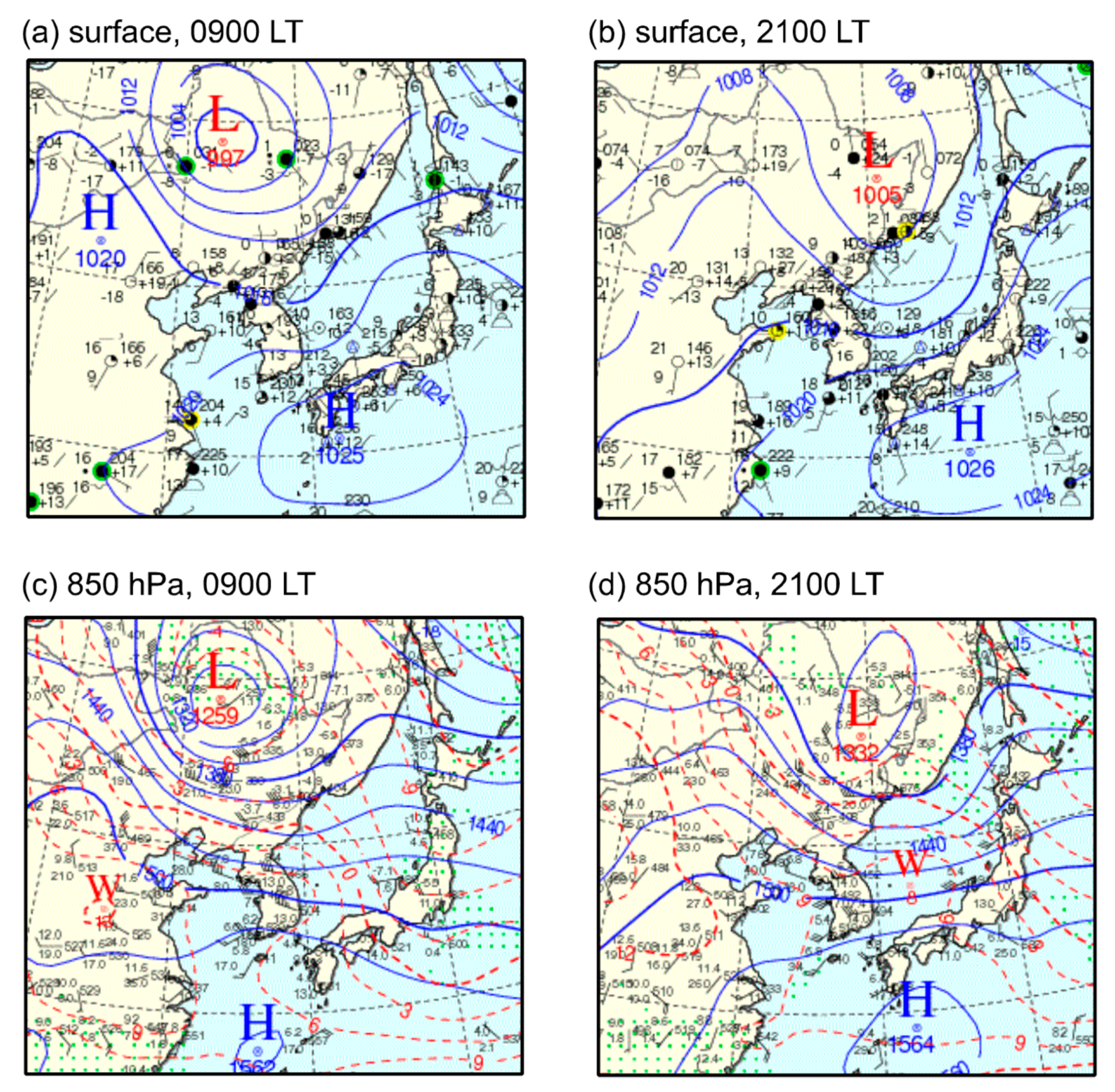
2. Synoptic Analysis

The 8 April 2012 windstorm case is analyzed in this study. Figure 1 shows the surface and 850-hPa weather charts at 0900 LT (local time = UTC + 9 h) and 2100 LT on this day. The locations of Yangyang, Jangjeon, Uljin, and Osan stations and topographic features are shown in Figure 2b. At 0900 LT, which is a time before the maximum instantaneous wind speed is observed at Yangyang station, the low and high pressure systems are located north and south of the Korean Peninsula, respectively (Figure 1a). This synoptic pressure pattern is favorable for strong westerly winds in spring. The analysis of radiosonde data at Osan, an upstream station, reveals that the prevailing wind direction in the lower atmosphere on 8 April 2012 is westerly to southwesterly, so it is almost perpendicular to the ridge line of the Taebaek Mountains which is elongated approximately in the northwest-southeast direction in the middle eastern part of South Korea. This is a good condition for the generation of downslope windstorms. The northern low moves southeastward, and the southern high moves eastward. The pressure gradient in the middle eastern part of South Korea becomes larger at 2100 LT (Figure 1b). The 850-hPa weather charts (Figure 1c,d) also show a similar synoptic pressure pattern. In addition, the 850-hPa temperature becomes high over South Korea with time (Figure 1c,d), indicating the 850-hPa level near the mountain top height becomes more stable.
On 8 April 2012, the 10-m maximum instantaneous wind speed is 11.3 m s−1 at Osan station and 22.2 m s−1 at Yangyang station, showing a large difference in wind speed between the upstream and downstream stations of the Taebaek Mountains. This implies that the strong winds on the lee side are directly related to the mountain.

3. Model and Simulation Design

In this study, the Weather Research and Forecasting (WRF) model version 3.8.1 [21] is used to simulate the windstorms. The model domain configuration, the terrain height in the innermost domain, and the areas and cross-section lines for analysis are presented in Figure 2. Five nested domains centered on the Yeongdong region are considered. The horizontal resolutions of domains 1, 2, 3, 4, and 5 are 27 km (160 × 160 grid points), 9 km (331 × 331), 3 km (601 × 601), 1 km (901 × 901), and 333 m (1000 × 1000), respectively. There are 59 layers in the vertical direction. The vertical grid size, which is stretched with height, is ~70 m in the lowest model layer and ~410 m in the highest model layer. The time steps for domains 1, 2, 3, 4, and 5 are 60, 20, 6.66, 2.22, and 0.3 s, respectively. The model is integrated over 36 h from 2100 LT on 7 April to 0900 LT on 9 April 2012, and the data on 8 April 2012 are analyzed.
For the initial and boundary conditions, the ERA interim reanalysis data with 0.75° horizontal resolution [22] are used. The Shuttle Radar Topography Mission (SRTM) data with a resolution of 3˝ are used to represent fine-scale topographic features [23]. The following physical parameterization schemes are selected for the windstorm simulation: the Mellor-Yamada-Janjić planetary boundary layer scheme [24], the unified Noah land surface model [25], the WRF single-moment 6-class cloud microphysics scheme [26], the Dudhia shortwave radiation scheme [27], the Rapid Radiative Transfer Model (RRTM) longwave radiation scheme [28], and the Kain–Fritsch cumulus convection scheme [29], which is applied only to domains 1 and 2.

4. Results and Discussion
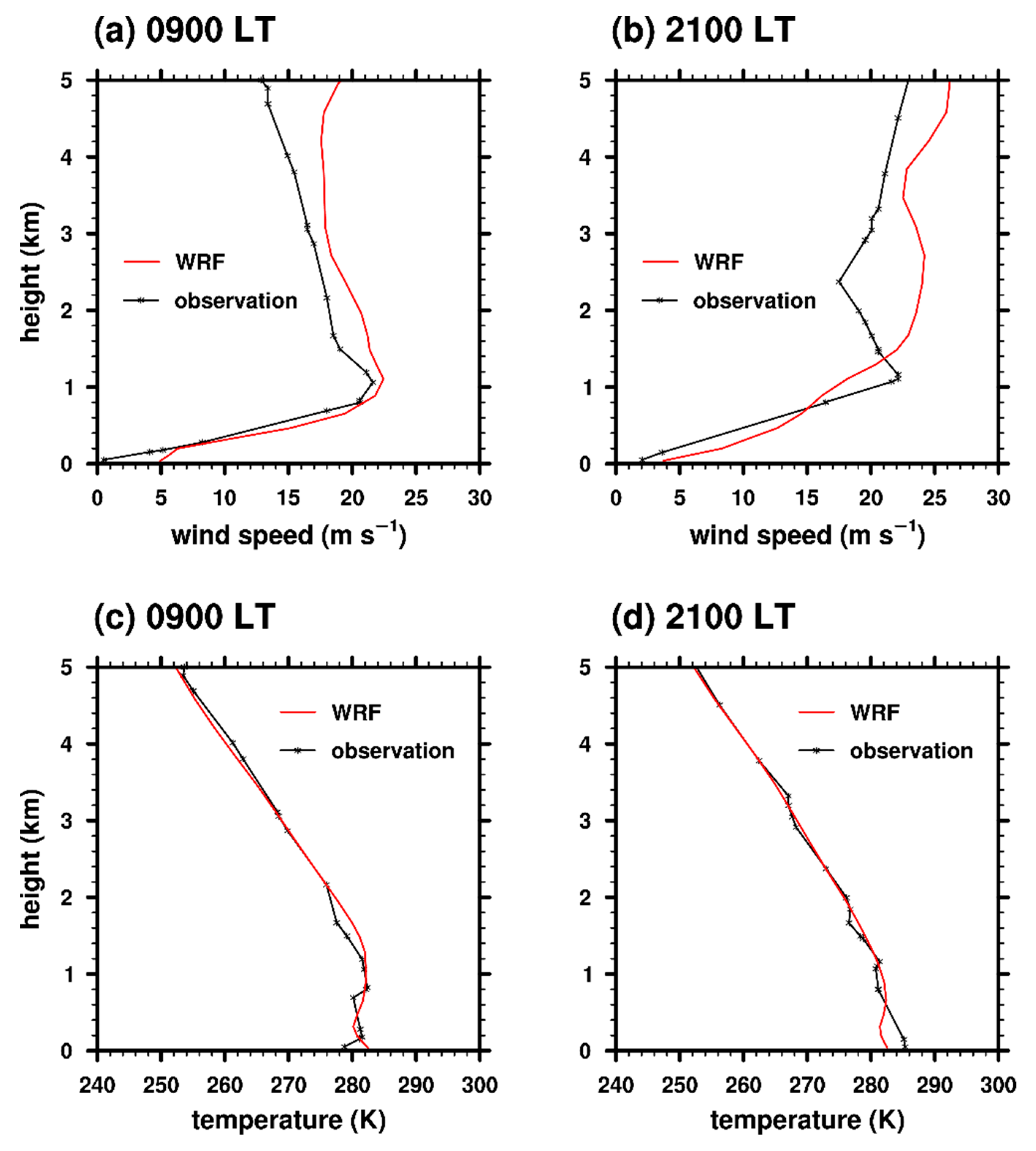
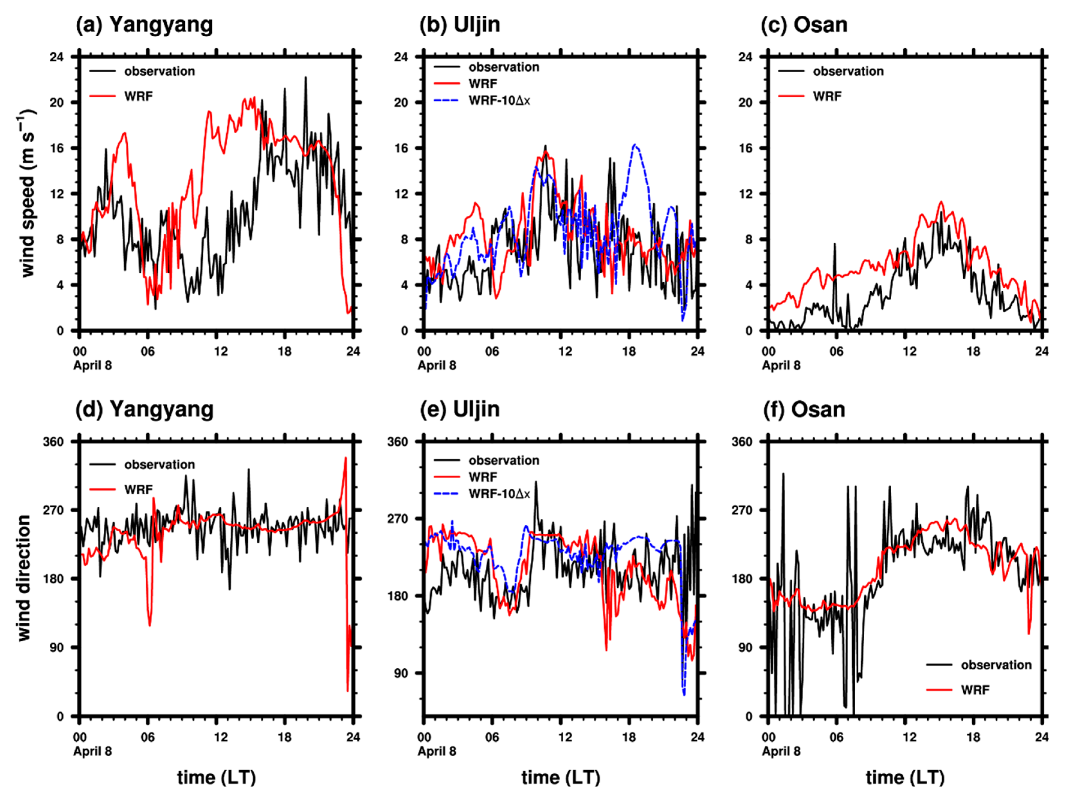
4.1. Validation

Using radiosonde data at Osan station, which is located at the upwind side of the area of interest, the vertical profiles of the simulated wind speed and air temperature are validated (Figure 3). At 0900 LT, although the WRF model overestimates the wind speed above a height of ~1 km, the simulated wind speed profile is similar to the observed profile. The model also reproduces the temperature profile well. The WRF results and observation both show the elevated inversion layer below a height of ~1 km, and the simulated inversion layer is thicker than the observed inversion layer. It seems that the difference of the inversion layer thickness is to some extent caused by the different vertical resolutions of the radiosonde data and WRF model. Below a height of ~1 km, the vertical resolution of the WRF model stretches with height from ~70 m to ~200 m, but the vertical resolution of the radiosonde data varies irregularly from ~20 m to ~400 m. At 2100 LT, the simulated wind speed above a height of ~1.5 km is slightly higher than the observation. The overall pattern of the simulated wind speed is similar to the observation. The simulated temperature profile is also well matched with the observed one, except below a height of ~500 m.
Figure 4 shows the time series of the 10-m instantaneous wind speed and wind direction at Yangyang, Uljin, and Osan stations. At Yangyang station, there are two periods in which strong winds appear in both the observation and the simulation: around 0300 LT and 1800 LT on 8 April. The maximum wind speed in the first period is 15.9 m s−1 at 0220 LT in the observation, and it is 17.3 m s−1 at 0400 LT in the simulation. In the first period, the model well simulates the maximum wind speed which is 1.4 m s−1 stronger and occur 1 h 40 m later compared to the observation. The maximum wind speed in the second period is 22.2 m s−1 at 1950 LT in the observation, and it is 20.5 m s−1 at 1520 LT in the simulation. The maximum wind in the second period is simulated to be 1.7 m s−1 weaker and occur 4 h 30 m earlier compared to the observation. The reason for the shift in the maximum wind speed can be attributed to the fact that the upwind flow in the simulation is enhanced earlier than that in the observation. The simulated 10-m wind direction is well matched with the observed one. The wind direction at Yangyang station is mainly westerly to southwesterly for both the simulation and the observation.
The observed 10-m instantaneous wind speed at Uljin station is generally weaker than that at Yangyang station. However, the strong winds at Uljin station also appear in two periods on 8 April. The strong winds in the first period appear around 1040 LT in both the observation and the simulation. The model simulates the maximum wind speed in the first period as 15.7 m s−1, which is very close to the observed value of 16.2 m s−1. However, the maximum wind speed in the second period, which is 15.1 m s−1 at 1620 LT in the observation, fails to be simulated. The reasons for this will be explained in Section 4.5. The wind direction at Uljin station is southerly to southwesterly for both the simulation and the observation.
Osan station, located at the upwind side, has relatively low 10-m wind speed compared to Yangyang and Uljin stations. It clearly shows that the wind speed increases in the downwind side of the mountains like Yangyang and Uljin stations. The model reproduces this wind speed difference well. Although the observed high-frequency fluctuation of the 10-m wind direction does not appear in the simulation, the model well simulates the overall trend of the 10-m wind direction at Osan station.
Although there are some limitations in simulating the maximum wind speeds at Yangyang and Uljin stations, they are simulated within an error of 2 m s−1 in wind speed, except for the maximum wind speed in the second period at Uljin station. The overall trend of the simulated 10-m wind speed is also similar to the observed one, although the maximum wind speed at Yangyang station appears at different times in the simulation and observation. The 10-m wind direction shows a good agreement between the simulation and the observation. Thus, it would be appropriate to examine the characteristics of the 8 April 2012 windstorms and their generation mechanisms using the simulation data.

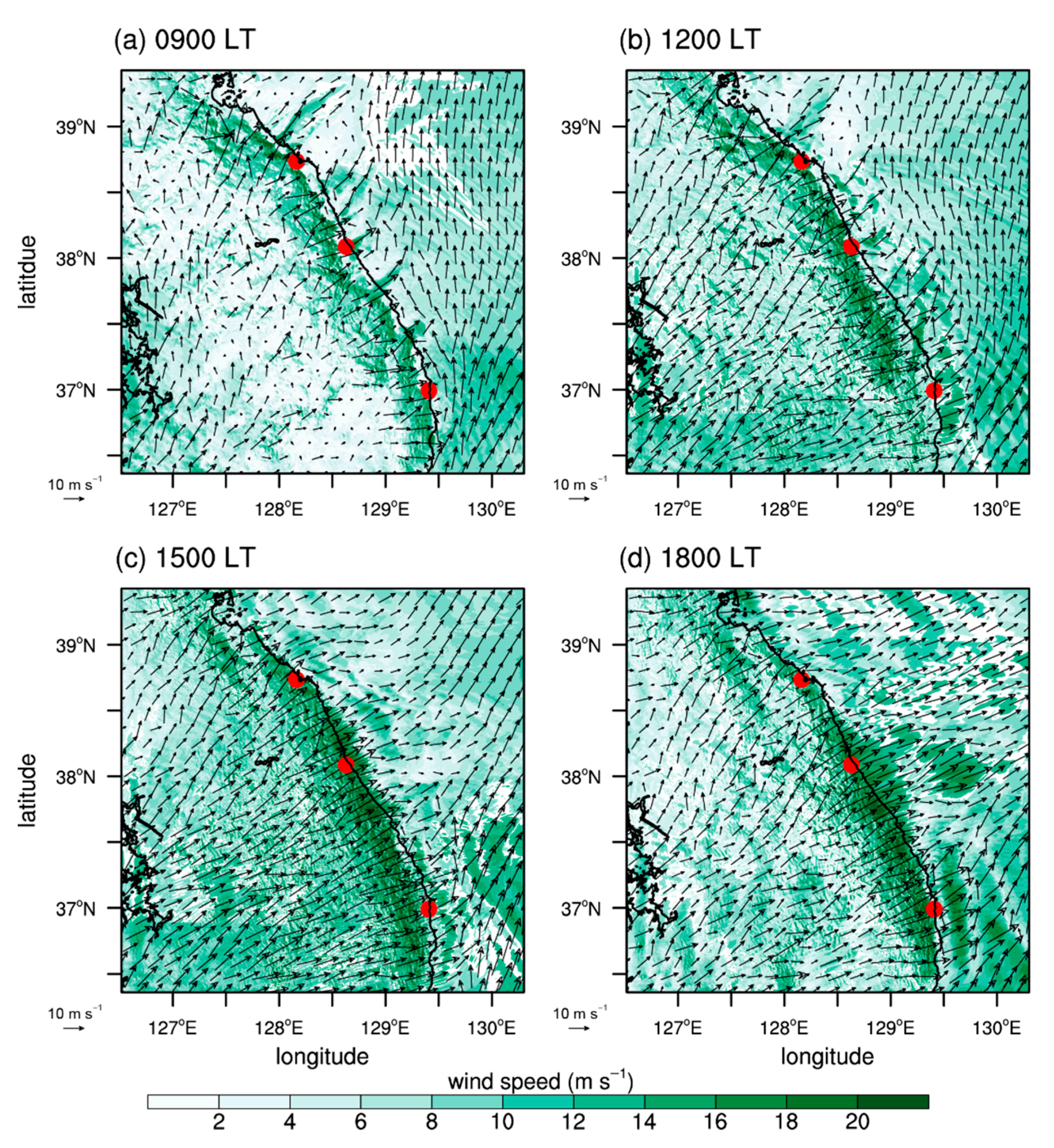
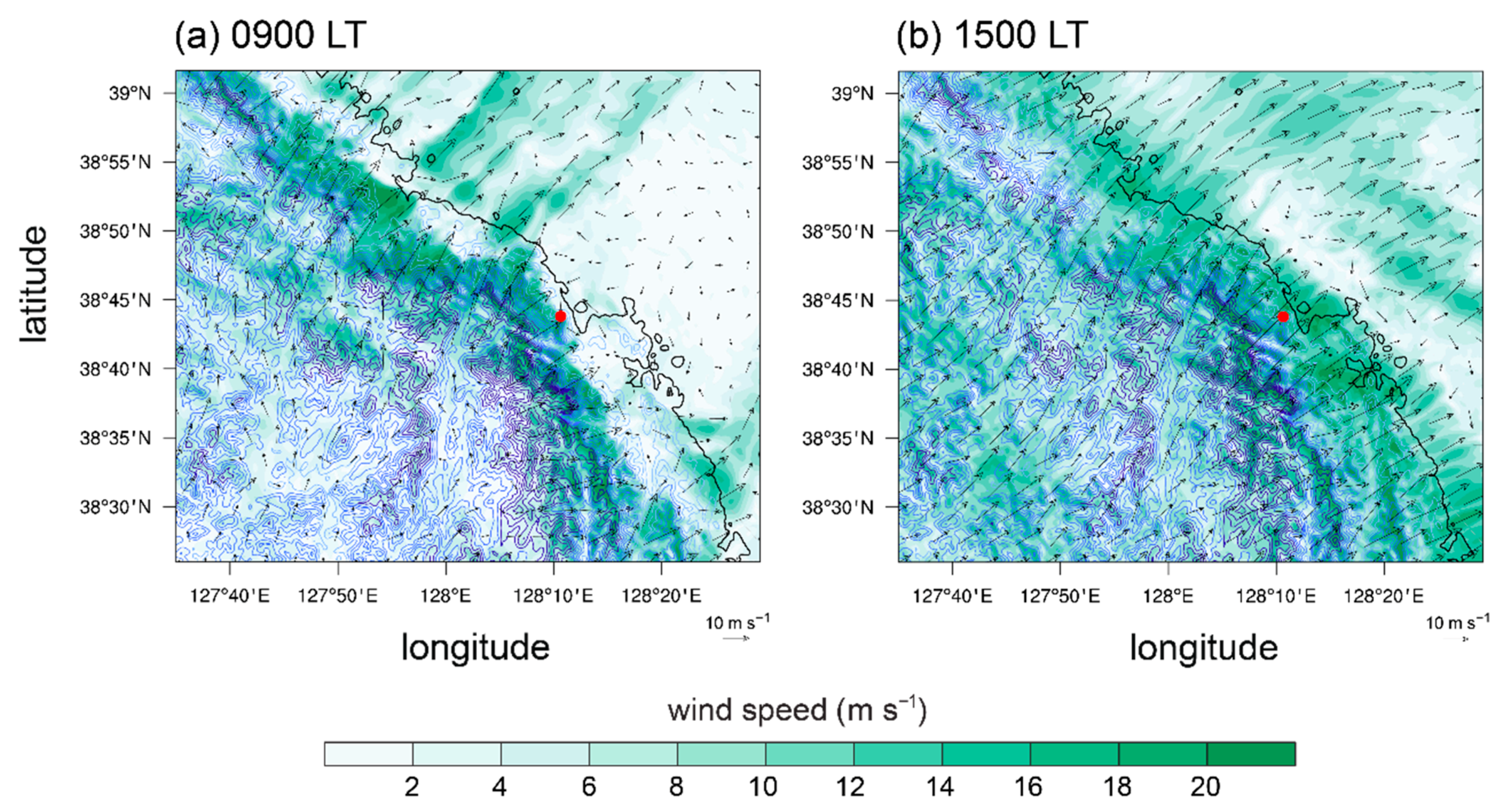
4.2. Overall Characteristics of the Simulated Winds

To see the overall characteristics of the simulated winds, the 10-m wind speed and wind vector in the innermost domain are analyzed (Figure 5). At 0900 LT on 8 April, the winds are relatively strong on the lee slope of the Taebaek Mountains (Figure 5a). The winds on the windward side of the mountain range are relatively weak. On the lee of the mountain range, there are areas of plume-shaped wind pattern extending seaward, particularly noticeable north of Jangjeon station. In the East Sea/Sea of Japan, the southerly winds are predominant. At 1200 LT, the winds on the windward side become stronger than at 0900 LT and the winds blow approximately perpendicular to the mountain range (Figure 5b). This is largely because of the enhanced prevailing winds associated with the northern low and southern high (see Figure 1). Additionally, severe downslope windstorms in the lee of the Taebaek Mountains are clearly evident. At 1500 LT, just before the simulated maximum 10-m wind speed appears at Yangyang station, the windstorm along the Taebaek Mountains is extended seaward and intensified (Figure 5c). At 1800 LT, the banded pattern of strong-wind regions and weak-wind regions, which is parallel to the coastal line, appears near Uljin (Figure 5d).
To examine these characteristics in detail, we zoom in on three areas to take advantage of the high-resolution simulation; (1) Yangyang area for which we focus on the downslope windstorm (C1 in Figure 2b), (2) Jangjeon area for which we focus on the plume-shaped wind pattern (A1 in Figure 2b), and (3) Uljin area for which we focus on the banded wind pattern (A2 and C2 in Figure 2b).

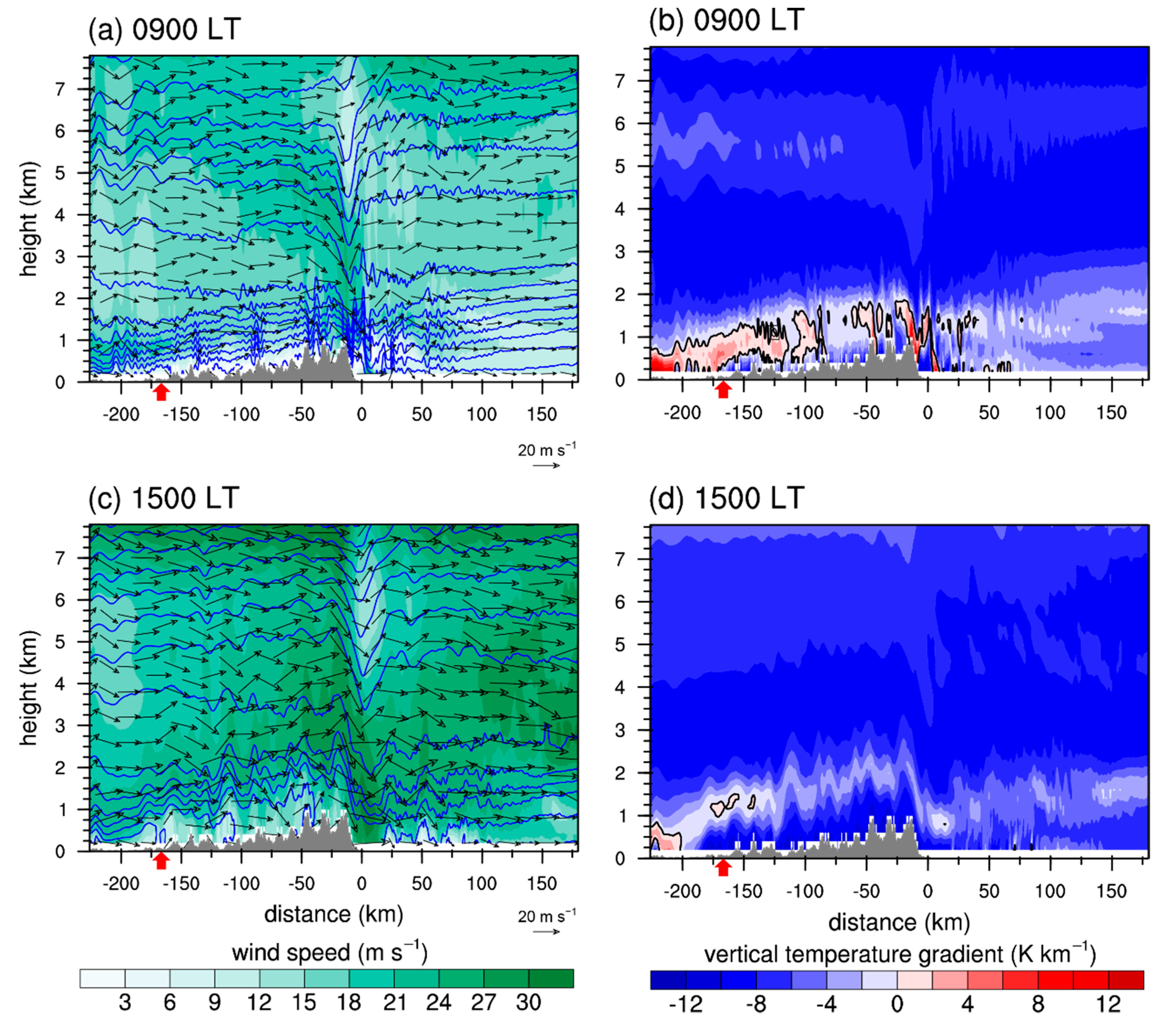
4.3. Downslope Windstorm (Yangyang)

For the analysis of the downslope windstorm in the Yangyang area, potential temperature, wind speed, wind vector, and vertical temperature gradient at 0900 LT and 1500 LT are plotted in the vertical cross-section along C1 in Figure 2b (Figure 6). Note that the location of Osan station is denoted by the red arrow in Figure 6. At 0900 LT, the downslope windstorm appears along/over the downslope of the Taebaek Mountains (Figure 6a). The isentropes (potential temperature isolines) descend steeply on the lee slope of the mountain and recover farther leeward. This structure of isentropes suggests that the hydraulic jump is responsible for the downslope windstorm in the Yangyang area. In addition, the jump-like motion of the inversion layer over the downslope of the mountain shows that the hydraulic jump is involved in the downslope windstorm (Figure 6b) [30,31]. The downslope windstorm is enhanced in the lee of the mountain range at 1500 LT, and the structure of hydraulic jump propagates leeward, passing Yangyang station. These correspond to the rapid increase of the 10-m wind speed at Yangyang from 0600 LT to 1500 LT (see Figure 4a).
The hydraulic jump in the Yangyang area is mainly caused by the elevated inversion near the mountain top height. At 0900 LT, the strong elevated inversions above the upslope and the ridge of the mountain range are clearly shown (Figure 6b). The elevated inversion can act as a free surface in the shallow water theory and help the atmospheric flow to undergo a transition from subcritical to supercritical flow [32]. At 1500 LT, the elevated inversion is dissipated because of diurnal heating in the daytime (Figure 6d) and the downslope windstorm is weakened after 1500 LT.
To quantitatively investigate atmospheric conditions for the formation of the hydraulic jump, the Fr-M diagram [33] is shown in Figure 7. The Froude number Fr and the dimensionless height M are given as follows:
F r = U g H ,
M = h m H .
Here, U is the wind speed, g′ = gΔθ/θ0 is the reduced gravity where g is the gravitational acceleration, Δθ is the potential temperature difference between the inversion layer top and the inversion layer bottom, and θ0 is the potential temperature, H is the inversion layer top height, and hm is the mountain top height. The inversion layer top (bottom) is defined by the highest (lowest) model level of the layer in which the vertical temperature gradient is positive. U and θ0 are averaged from the surface to the inversion layer top height. Note that U is the wind speed in the C1 direction in Figure 2b. The simulation data at the location of Osan station are used for the calculation, and the data without the inversion are excluded. The radiosonde data at Osan station are also used for the calculation. In the Fr-M diagram, regimes I, II, III, and IV represent subcritical flow, hydraulic jump, supercritical flow, and totally blocked flow, respectively. The Fr-M diagram (Figure 7) shows that the simulated incoming flows before 0400 LT, when downslope windstorm and the structure of hydraulic jump are not evident, are mainly in regime IV. After 0400 LT, the simulated incoming flows are in regime II. The observed incoming flows are in regime II for all times. These results imply that the incoming flows with a favorable condition for hydraulic jump play an important role in the formation of the downslope windstorm.
Additionally, an overall feature of the topography is that the topographic height increases gradually and then decreases rapidly in the downwind direction. This means that the leeward slope is much steeper than the windward slope. This topographic feature is also favorable for the downslope windstorm.
The critical-level reflection is not relevant as the generation mechanism for the downslope windstorm in the Yangyang area. Due to the strong prevailing winds resulting from the synoptic pressure pattern of the northern low and the southern high, it is difficult for a critical level to be self-induced. The climatological statistics of springtime windstorms in Gangneung, the Yeongdong region reveal that only 5% of the downslope windstorms are related to the critical-level reflection [18].
In the Yangyang area, the maximum wind speed appears earlier in the WRF model than the observation. However, this shift in the maximum wind speed of the WRF model (Figure 4a) non-significantly impacts the favorable conditions for the downslope windstorm discussed in this section (e.g., the elevated inversion layer near the mountain top height and the steeper leeward slope). Therefore, the generation mechanism of the downslope windstorm conjectured from these conditions remains unchanged.

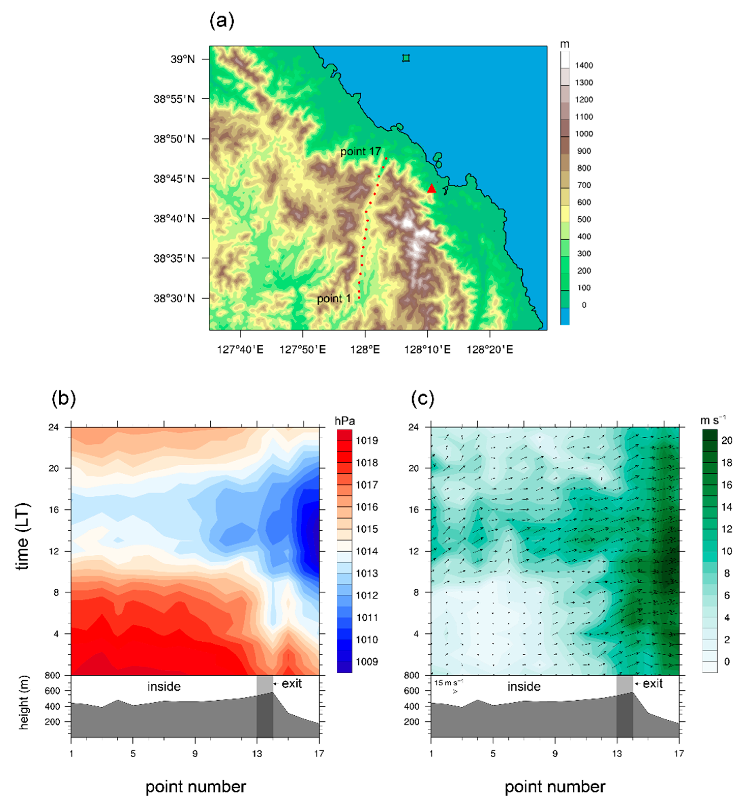
4.4. Gap Winds (Jangjeon)

Figure 8 shows the simulated 10-m wind fields at 0900 LT and 1500 LT in the Jangjeon area. At 0900 LT, just north of Jangjeon station, the area of the plume-shaped wind pattern extending seaward from the mountain gap is apparent (Figure 8a; see Figure 9a for the gap location). As the winds become strong along the coastal region with time, the plume-shaped wind pattern is less identifiable (Figure 8b). Notice that the strong windstorms appear on the lee slope of the Taebaek Mountains (Figure 8).
The decrease in the pressure near the exit of a gap is a mechanism for gap winds [34,35,36,37]. The present numerical simulation is suitable for revealing such a local pressure change because the high-resolution grid system and the high-resolution terrain data are used. The local pressure difference between the gap inside and the gap exit is analyzed using sea-level pressure at 17 points in and out of the gap (Figure 9a). The sea-level pressure and the 10-m wind speed along the 17 points are shown in Figure 9b,c. Before 0900 LT, the sea-level pressure differences are large and the local minimum of the sea-level pressure and the local maximum of the 10-m wind speed at the gap exit are clearly represented. Around 1500 LT, the differences of the sea-level pressure and the 10-m wind speed between the gap inside (points 1–12) and the gap exit (points 13–14) are smaller than around 0900 LT.
To examine the relationship between the sea-level pressure and the 10-m wind speed, the difference of the sea-level pressure and the 10-m wind speed between the gap inside and the gap exit are plotted in Figure 10. The values of the gap inside and the gap exit are averaged over the points 1–12 and the points 13–14, respectively. Around 0500 LT, the large sea-level pressure difference (−3.4 hPa) induces the large 10-m wind speed difference (~12 m s−1). It is well matched with the local maximum of 10-m wind speed at the gap exit (Figure 9c). When the sea-level pressure difference decreases with time from 0500 LT, the 10-m wind speed difference also decreases. However, the wind speed near the gap exit is similar to the one of early morning (Figure 9c). It is because the larger-scale synoptic pressure pattern increases the wind speed at the gap inside. Accordingly, a plume-shaped wind pattern, which is an indicative of the wind speed increase at the gap exit, appears better in the morning than in the afternoon.

4.5. Association with Planetary Boundary Layer (Uljin)

To analyze the banded wind pattern in the Uljin area, the 10-m wind and planetary boundary layer (PBL) height fields are plotted (Figure 11). In the Mellor-Yamda-Janjić PBL scheme, the PBL height is determined by the lowest model level above the surface at which TKE decreases to a prescribed lower bound. At 1800 LT, the well-defined-banded pattern of very strong-wind regions and weak-wind regions is evident. The banded wind pattern is parallel to the coastal line. In the strong- and weak-wind regions, the westerly and the southerly winds are prevailing, respectively. Comparison of the wind field and the PBL height field shows that in the banded wind pattern, the strong-wind region coincides with the region of shallower PBL, while the weak-wind region coincides with the region of deeper planetary boundary layer. This implies that strong winds can be related to PBL height.
To investigate the interaction between the downslope windstorm and the PBL, the potential temperature, wind speed, wind vector, and the bulk Richardson number smaller than 0.25 at 1800 LT are plotted in the vertical cross-section along C2 in Figure 2b (Figure 12). In the east of Uljin station, the weak-wind regions appear in the PBL and have low bulk Richardson number due to strong wind shear. The downslope windstorm does not penetrate the weak-wind region with low bulk Richardson number, but instead passes over it. The PBL height also follows this wavy flow pattern and is well matched with the weak-wind and low bulk Richardson number regions. As with a flow over a mountain, the wind speed increases on the downwind of these regions. The banded wind pattern appears as a result of the weak-wind regions and the increased wind speed on the downwind side of these regions.
The interaction between the PBL and the downslope windstorm is unclear. Some studies [38,39,40,41] show that the PBL absorbs downward reflected gravity waves, thus effectively limiting trapped mountain waves or significantly reducing the drag and momentum flux of mountain waves above. Accordingly, the strong windstorms due to wave-involved mechanisms can be weakened. However, the PBL as an effective mountain is reported [42,43,44]. According to these studies, mountain waves can be forced by an effective mountain, not by a real mountain only [42,43,44], and flow regime can also be influenced by the PBL height [43].
Considering those effects in the present study, the role of the PBL as an energy absorber is unclear. However, the height with maximum wind speed is near the PBL top height, not near the surface, suggesting that the PBL could act as an effective mountain [42]. The large vertical displacement of the isentropes above the PBL in the east of Uljin station and the windstorm appearing at the downslope of the PBL imply that the PBL could force gravity waves and change flow regime. However, the aforementioned features do not directly show the effects of the PBL on the windstorm. Additionally, it is not clear how the role of the PBL as an absorber and the PBL as an effective mountain differently affect the windstorm. Therefore, further in-depth research about the effects of the PBL on windstorms is needed.
The time variation of the observed wind speed at Uljin station (Figure 4b) can be explained by the banded wind pattern coupled with the spatiotemporal variation of the PBL height (Figure 13). As the deep PBL developed in the afternoon is pushed seaward, it passes over Uljin station and the wind speed decreases. After the deep PBL passes over Uljin station, the wind speed increases, because it is located upwind of the deep PBL. However, the WRF model failed, in location, to simulate this increase in wind speed well. The time variation of the simulated maximum wind speed at the location 3.33 km west of Uljin station, as illustrated by the blue dotted line in Figure 4b, reasonably simulates the observed strong winds at 1620 LT. After the strong winds at 1620 LT, the deep PBL returns to Uljin station, decreasing the wind speed there.

5. Summary and Conclusions

In this study, the characteristics and generation mechanisms of the windstorms occurring in the lee of the Taebaek mountain on 8 April 2012 were investigated using the high-resolution WRF model simulation. Three different areas (Yangyang, Jangjeon, and Uljin) were selected for the analysis. In the Yangyang area, the severe downslope windstorm in the lee of the Taebaek Mountains appears. The steep descent of the isentropes on the lee slope of the mountain and their recovery farther leeward are typical features of hydraulic jump. Inversion layers near the highest mountain top height and incoming flow in hydraulic jump regime support the hydraulic jump mechanism for the generation of the downslope windstorm. In the Jangjeon area, the plume-shaped wind pattern extending seaward from the exit of the gap is clearly seen. The gap winds are induced by the large pressure gradient between the inside and exit of the gap. In the Uljin area, the banded pattern of strong-wind regions and weak-wind regions is distinct. The banded wind pattern is parallel to the coastal line. Interestingly, we found that the strong-wind (weak-wind) region coincides with the region of shallower (deeper) planetary boundary layer and that in the weak-wind region, the southerly winds are prevailing. This is because the downslope windstorm does not penetrate the weak-wind region with low bulk Richardson number and passes over it. The windstorms and their features are well simulated in our simulation with the gray-zone resolution (Δx = 333 m). However, we need a scale-aware PBL parameterization or a large-eddy simulation to better simulate the fine structure and evolution of the windstorms.
In this study, we showed that even if windstorms directly related to topography occur on the same day, their generation mechanisms can differ depending on the local topographic features. This suggests that even under the same synoptic conditions, local topographic features should be taken into consideration in forecasting windstorms in mountainous regions.

Author Contributions

J.L. conducted the numerical simulation and prepared the figures. J.L., J.M.S., J.-J.B., S.-B.P., and B.-S.H. contributed to the analysis and interpretation of the numerical simulation results. J.L., J.-J.B., and B.-S.H. wrote the manuscript. All authors have read and agreed to the published version of the manuscript.

Funding

This work was supported by the Research Institute of Basic Sciences funded by the National Research Foundation of Korea (NRF-2019R1A6A1A10073437).

Acknowledgments

The authors are grateful to two anonymous reviewers for providing valuable comments on this study. The authors thank the supercomputer management division of the Korea Meteorological Administration for providing us with the supercomputer resource.

Conflicts of Interest

The authors declare no conflicts of interest.

References

  1. Lin, Y.-L. Mesoscale Dynamics; Cambridge University Press: Cambridge, UK, 2007; p. 630. [Google Scholar]
  2. Durran, D.R. Mountain waves and downslope winds. In Atmospheric Processes over Complex Terrain; Meteorological Monographs; American Meteorological Society: Boston, MA, USA, 1990; Volume 23, pp. 59–81. [Google Scholar]
  3. Long, R.R. Some aspects of the flow of stratified fluids: I. A theoretical investigation. Tellus 1953, 5, 42–58. [Google Scholar] [CrossRef] [Green Version]
  4. Eliassen, A.; Palm, E. On the transfer of energy in stationary mountain waves. Geofys. Publ. 1960, 22, 1–23. [Google Scholar]
  5. Klemp, J.B.; Lilly, D.R. The dynamics of wave-induced downslope winds. J. Atmos. Sci. 1975, 32, 320–339. [Google Scholar] [CrossRef] [Green Version]
  6. Clark, T.L.; Peltier, W.R. Critical level reflection and the resonant growth of nonlinear mountain waves. J. Atmos. Sci. 1984, 41, 3122–3134. [Google Scholar] [CrossRef]
  7. Reed, T.R. Gap winds of the Strait of Juan de Fuca. Mon. Weather Rev. 1931, 59, 373–376. [Google Scholar] [CrossRef]
  8. Colle, B.A.; Mass, C.F. High-resolution observations and numerical simulations of easterly gap flow through the Strait of Juan de Fuca on 9–10 December 1995. Mon. Weather Rev. 2000, 128, 2398–2422. [Google Scholar] [CrossRef]
  9. Sharp, J.; Mass, C. Columbia Gorge gap flow: Insights from observational analysis and ultra-high-resolution simulation. Bull. Am. Meteorol. Soc. 2002, 83, 1757–1762. [Google Scholar] [CrossRef]
  10. Decker, S.G.; Robinson, D.A. Unexpected high winds in northern New Jersey: A downslope windstorm in modest topography. Weather Forecast. 2011, 26, 902–921. [Google Scholar] [CrossRef]
  11. Ágústsson, H.; Ólafsson, H. The bimodal downslope windstorms at Kvísker. Meteorol. Atmos. Phys. 2012, 116, 27–42. [Google Scholar] [CrossRef]
  12. Mofidi, A.; Soltanzadeh, I.; Yousefi, Y.; Zarrin, A.; Soltani, M.; Samakosh, J.M.; Azizi, G.; Miller, S.T.K. Modeling the exceptional south Foehn event (Garmij) over the Alborz Mountains during the extreme forest fire of December 2005. Nat. Hazards 2015, 75, 2489–2518. [Google Scholar] [CrossRef]
  13. Cao, Y.; Fovell, R.G. Downslope windstorms of San Diego County. Part I: A case study. Mon. Weather Rev. 2016, 144, 529–552. [Google Scholar] [CrossRef]
  14. Shestakova, A.A.; Moiseenko, K.B.; Toropov, P.A. Hydraulic and wave aspects of Novorossiysk Bora. Pure Appl. Geophys. 2018, 175, 3741–3757. [Google Scholar] [CrossRef]
  15. Tollinger, M.; Gohm, A.; Jonassen, M.O. Unravelling the March 1972 northwest Greenland windstorm with high-resolution numerical simulations. Q. J. R. Meteorol. Soc. 2019, 145, 3409–3431. [Google Scholar] [CrossRef] [Green Version]
  16. Vosper, S.B. Inversion effects on mountain lee waves. Q. J. R. Meteorol. Soc. 2004, 130, 1723–1748. [Google Scholar] [CrossRef]
  17. Lee, J.G. A numerical study of the orographic effect of the Taebak mountains on the increase of the downslope wind speed near Gangnung area. J. Environ. Sci. 2003, 12, 1245–1254, (In Korean with English Abstract). [Google Scholar]
  18. Jang, W.; Chun, H.-Y. Severe downslope windstorms of Gangneung in the springtime. Atmosphere 2008, 18, 207–224, (In Korean with English Abstract). [Google Scholar]
  19. Lee, J.G.; In, S.-R. A numerical sensitivity experiment of the downslope windstorm over the Yeongdong region in relation to the inversion layer of temperature. Atmosphere 2009, 19, 331–344, (In Korean with English Abstract). [Google Scholar]
  20. Korea Meteorological Administration. Meteorological Information Portal Service System Disaster Prevention. Available online: https://afso.kma.go.kr (accessed on 22 November 2019).
  21. Skamarock, W.C.; Klemp, J.B.; Dudhia, J.; Gill, D.O.; Barker, D.M.; Duda, M.G.; Huang, X.-Y.; Wang, W.; Powers, J.G. A Description of the Advanced Research WRF Version 3; Technical Report TN-475+STR; NCAR: Boulder, CO, USA, 2008. [Google Scholar]
  22. Dee, D.P.; Uppala, S.M.; Simmons, A.J.; Berrisford, P.; Poli, P.; Kobayashi, S.; Andrae, U.; Balmaseda, M.A.; Balsamo, G.; Bauer, P.; et al. The ERA-Interim reanalysis: Configuration and performance of the data assimilation system. Q. J. R. Meteorol. Soc. 2011, 137, 553–597. [Google Scholar] [CrossRef]
  23. Jarvis, A.; Guevara, E.; Reuter, H.I.; Nelson, A.D. Hole-Filled SRTM for the Globe: Version 4: Data Grid; CGIAR Consortium for Spatial Information: Washington, DC, USA, 2008. [Google Scholar]
  24. Janjić, Z.I. The step-mountain eta coordinate model: Further developments of the convection, viscous sublayer, and turbulence closure schemes. Mon. Weather Rev. 1994, 122, 927–945. [Google Scholar] [CrossRef] [Green Version]
  25. Tewari, M.; Chen, F.; Wang, W.; Dudhia, J.; LeMone, M.A.; Mitchell, K.; Ek, M.; Gayno, G.; Wegiel, J.; Cuenca, R.H. Implementation and verification of the unified NOAH land surface model in the WRF model. In Proceedings of the 20th Conference on Weather Analysis and Forecasting, 16th Conference on Numerical Weather Prediction, Seattle, WA, USA, 14 January 2004. [Google Scholar]
  26. Hong, S.-Y.; Lim, J.-O.J. The WRF single-moment 6-class microphysics scheme (WSM6). J. Korean Meteorol. Soc. 2006, 42, 129–151. [Google Scholar]
  27. Dudhia, J. Numerical study of convection observed during the Winter Monsoon Experiment using a mesoscale two-dimensional model. J. Atmos. Sci. 1989, 46, 3077–3107. [Google Scholar] [CrossRef]
  28. Mlawer, E.J.; Taubman, S.J.; Brown, P.D.; Iacono, M.J.; Clough, S.A. Radiative transfer for inhomogeneous atmospheres: RRTM, a validated correlated-k model for the longwave. J. Geophys. Res. 1997, 102, 16663–16682. [Google Scholar] [CrossRef] [Green Version]
  29. Kain, J.S. The Kain–Fritsch convective parameterization: An update. J. Appl. Meteorol. 2004, 43, 170–181. [Google Scholar] [CrossRef] [Green Version]
  30. Klemp, J.B.; Durran, D.R. Numerical modelling of Bora winds. Meteorol. Atmos. Phys. 1987, 36, 215–227. [Google Scholar] [CrossRef]
  31. Smith, C.M.; Skyllingstad, E.D. Effects of inversion height and surface heat flux on downslope windstorms. Mon. Weather Rev. 2011, 139, 3750–3764. [Google Scholar] [CrossRef] [Green Version]
  32. Durran, D.R. Another look at downslope windstorms. Part I: The development of analogs to supercritical flow in an infinitely deep, continuously stratified fluid. J. Atmos. Sci. 1986, 43, 2527–2543. [Google Scholar] [CrossRef]
  33. Houghton, D.D.; Kasahara, A. Nonlinear shallow fluid flow over an isolated ridge. Commun. Pure Appl. Math. 1968, 21, 1–23. [Google Scholar] [CrossRef]
  34. Overland, J.E.; Walter, B.A., Jr. Gap winds in the Strait of Juan de Fuca. Mon. Weather Rev. 1981, 109, 2221–2233. [Google Scholar] [CrossRef] [Green Version]
  35. Mass, C.F.; Businger, S.; Albright, M.D.; Tucker, Z.A. A windstorm in the lee of a gap in a coastal mountain barrier. Mon. Weather Rev. 1995, 123, 315–331. [Google Scholar] [CrossRef] [Green Version]
  36. Armi, L.; Mayr, G.J. Continuously stratified flows across an Alpine crest with a pass: Shallow and deep föhn. Q. J. R. Meteorol. Soc. 2007, 133, 459–477. [Google Scholar] [CrossRef]
  37. Ohashi, Y.; Terao, T.; Shigeta, Y.; Ohsawa, T. In situ observational research of the gap wind “Hijikawa-Arashi” in Japan. Meteorol. Atmos. Phys. 2015, 127, 33–48. [Google Scholar] [CrossRef]
  38. Jiang, Q.; Doyle, J.D.; Smith, R.B. Interaction between trapped waves and boundary layers. J. Atmos. Sci. 2006, 63, 617–633. [Google Scholar] [CrossRef]
  39. Smith, R.B.; Jiang, Q.; Doyle, J.D. A theory of gravity wave absorption by a boundary layer. J. Atmos. Sci. 2006, 63, 774–781. [Google Scholar] [CrossRef]
  40. Smith, R.B. Interacting mountain waves and boundary layers. J. Atmos. Sci. 2007, 64, 594–607. [Google Scholar] [CrossRef]
  41. Jiang, Q.; Doyle, J.D. On the diurnal variation of mountain waves. J. Atmos. Sci. 2008, 65, 1360–1377. [Google Scholar] [CrossRef]
  42. Peng, M.S.; Thompson, W.T. Some aspects of the effect of surface friction on flows over mountains. Q. J. R. Meteorol. Soc. 2003, 129, 2527–2557. [Google Scholar] [CrossRef]
  43. Sauer, J.A.; Muñoz-Esparza, D.; Canfield, J.M.; Costigan, K.R.; Linn, R.R.; Kim, Y.-J. A large-eddy simulation study of atmospheric boundary layer influence on stratified flows over terrain. J. Atmos. Sci. 2016, 73, 2615–2632. [Google Scholar] [CrossRef]
  44. Worthington, R.M. Existence of large turbulent eddies in the early-morning boundary layer acting as an effective mountain to force mountain waves. Bound.-Layer Meteorol. 2016, 159, 161–172. [Google Scholar] [CrossRef]
Figure 1. Surface weather charts at (a) 0900 LT and (b) 2100 LT and 850-hPa weather charts at (c) 0900 LT and (d) 2100 LT on 8 April 2012. In (a,b), the mean sea-level pressure (blue solid lines) is contoured in 4 hPa intervals. In (c,d), the geopotential height (blue solid lines) is contoured in 30 gpm intervals and the temperature (red dashed lines) is contoured in 3 °C intervals. These weather charts are provided by the Korea Meteorological Administration [20]. The yellow and green marks on the cloud coverage symbol in (a,b) represent the fog and rain, respectively.
Atmosphere 11 00431 g001
Figure 2. (a) Five nested domains and (b) terrain height (m) in the innermost domain (domain 5). The areas enclosed by the red lines, A1 and A2, include Jangjeon and Uljin stations. The red solid lines C1 and C2 are passing Yangyang and Osan stations and Uljin station, respectively.
Atmosphere 11 00431 g002
Figure 3. Vertical profiles of wind speeds at (a) 0900 LT and (b) 2100 LT and temperatures at (c) 0900 LT and (d) 2100 LT at Osan station. The black and red lines indicate the radiosonde observation data and WRF simulation data, respectively.
Atmosphere 11 00431 g003
Figure 4. Time series of (ac) the 10-m instantaneous wind speed and (df) the 10-m instantaneous wind direction at (a,d) Yangyang, (b,e) Uljin, and (c,f) Osan stations. The black and red lines indicate the observed data and simulation results, respectively. The blue dashed line in (b,e) indicates the time series of the simulated 10-m wind speed and the wind direction at the location 10Δx (3.33 km) west of Uljin station.
Atmosphere 11 00431 g004
Figure 5. Simulated 10-m wind speed and wind vector fields at (a) 0900 LT, (b) 1200 LT, (c) 1500 LT, and (d) 1800 LT. The red dots indicate the locations of Jangjeon, Yangyang, and Uljin stations.
Atmosphere 11 00431 g005
Figure 6. Vertical cross-sections of the potential temperature (blue lines in a,c), wind speed (a,c), wind vector (a,c), and vertical temperature gradient (b,d) along C1 at (a,b) 0900 LT and (c,d) 1500 LT. The reference point on the horizontal axis (0 km) indicates the location of Yangyang station. The red arrow on the horizontal axis indicates the location of Osan station. The zero vertical temperature gradient lines are indicated by black lines.
Atmosphere 11 00431 g006
Figure 7. Diagram for asymptotic solutions to shallow water flow over an isolated obstacle as a function of the Froude number and dimensionless height. The red and black dots (stars) represent the condition of simulated (observed) incoming flow before 0400 LT and after 0400 LT, respectively. 69 samples in the simulation and 4 observed samples are used for this diagram.
Atmosphere 11 00431 g007
Figure 8. Simulated 10-m wind speed and the wind vector fields in A1 at (a) 0900 LT and (b) 1500 LT. The terrain height (blue lines) is contoured up to 1500 m in intervals of 100 m. The red circle indicates the location of Jangjeon station.
Atmosphere 11 00431 g008
Figure 9. (a) Terrain height (m) in A1. Hovmöller diagrams of the (b) sea-level pressure and (c) 10-m wind speed and 10-m wind vector at the 17 points. The red dots in Figure 9a indicate the selected 17 points in the gap. Vertical cross sections of the terrain height at the 17 points are added in the lower panels of Figure 9b,c. The red triangle indicates the location of Jangjeon station.
Atmosphere 11 00431 g009
Figure 10. Time series of the sea-level pressure (blue line) and the 10-m wind speed (black line) differences between the gap inside and the gap exit. The values of the gap inside and the gap exit are averaged over points 1–12 and points 13–14, respectively.
Atmosphere 11 00431 g010
Figure 11. Simulated (a) 10-m wind speed and wind vector fields and (b) planetary boundary layer height field in A2 at 1800 LT. The red dot indicates the location of Uljin station.
Atmosphere 11 00431 g011
Figure 12. Vertical cross-section of the wind speed, wind vector, potential temperature (blue lines), and bulk Richardson number smaller than 0.25 (black hatch lines) along C2 at 1800 LT. The PBL height is represented by magenta line. The reference point on the horizontal axis (0 km) indicates the location of Uljin station.
Atmosphere 11 00431 g012
Figure 13. Hovmöller diagram for the simulated planetary boundary layer height along C2. The black solid line indicates the location of Uljin station.
Atmosphere 11 00431 g013

