Neutrino Physics and Astrophysics with the JUNO Detector


Dipartimento di Fisica, Universitá degli Studi di Milano and I.N.F.N. Sezione di Milano, Via Celoria 16, 20133 Milano, Italy
Universe 2018, 4(11), 126; https://doi.org/10.3390/universe4110126
Submission received: 12 October 2018
/
Revised: 7 November 2018
/
Accepted: 13 November 2018
/
Published: 16 November 2018
(This article belongs to the Special Issue Selected Papers from the 7th International Conference on New Frontiers in Physics (ICNFP 2018))
Abstract
:The Jiangmen Underground Neutrino Observatory (JUNO) is a 20 kton liquid scintillator multi-purpose underground detector, under construction near the Chinese city of Jiangmen, with data collection expected to start in 2021. The main goal of the experiment is the neutrino mass hierarchy determination, with more than three sigma significance, and the high-precision neutrino oscillation parameter measurements, detecting electron anti-neutrinos emitted from two nearby (baseline of about 53 km) nuclear power plants. Besides, the unprecedented liquid scintillator-type detector performance in target mass, energy resolution, energy calibration precision, and low-energy threshold features a rich physics program for the detection of low-energy astrophysical neutrinos, such as galactic core-collapse supernova neutrinos, solar neutrinos, and geo-neutrinos.
1. Introduction, How to Infer the Mass Hierarchy
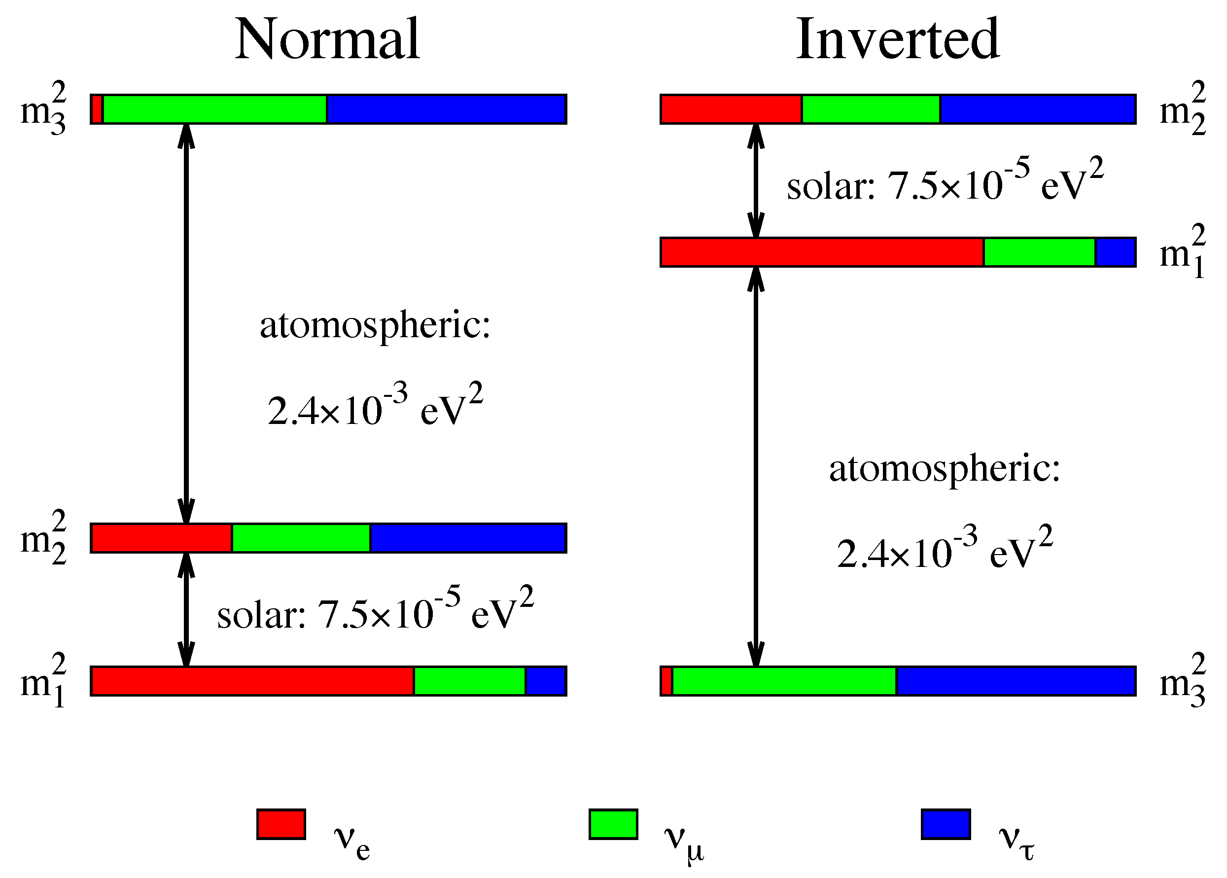
Among the remaining undetermined fundamental aspects in the leptonic sector of the standard model, there is the neutrino mass hierarchy (MH) determination (i.e., whether the neutrino mass eigenstate is heavier or lighter than the and mass eigenstates). The mass hierarchy discrimination will have an impact in the quest for the nature of the neutrino (Dirac or Majorana) [1]. The two possible scenarios, still compatible with the huge amount of data from different classes of neutrino experiments, usually denoted as normal and inverse hierarchy (NH and IH), are represented in Figure 1. Denoting the squared mass eigenvalues differences as , in the normal hierarchy case the third neutrino mass eigenvalue would be the biggest one and . Instead, in the inverted hierarchy case, would be the smallest eigenvalue and the relation would be . According to the most recent global analyses, the squared mass differences are1:
The relatively high value of the angle, ( = 8.46, at for the normal hierarchy [3]) makes possible the realization of the idea [4,5] to extract the mass hierarchy from the study of hierarchy-dependent oscillation probability corrections, which are proportional to sin .
We can write the survival probability in the form2:
The last term of Equation (3), indicated as , represents the mass hierarchy-dependent contribution to the oscillation probability. It can be rewritten as:
where represents the combination = ( + ). The new quantity is defined in such a way that sin and are combinations of the mass and mixing parameters in the 1–2 sector3. The ± sign in the last term of Equation (4) is decided by the MH, with plus sign for the normal one and minus sign for the inverted one. Hence, the survival (or oscillation) probability and consequently the observed spectrum are characterized by the presence of rapidly oscillating terms. Phases are in opposition for the two MH cases (NH and IH), superimposed to the general oscillation pattern valid for both hierarchies.
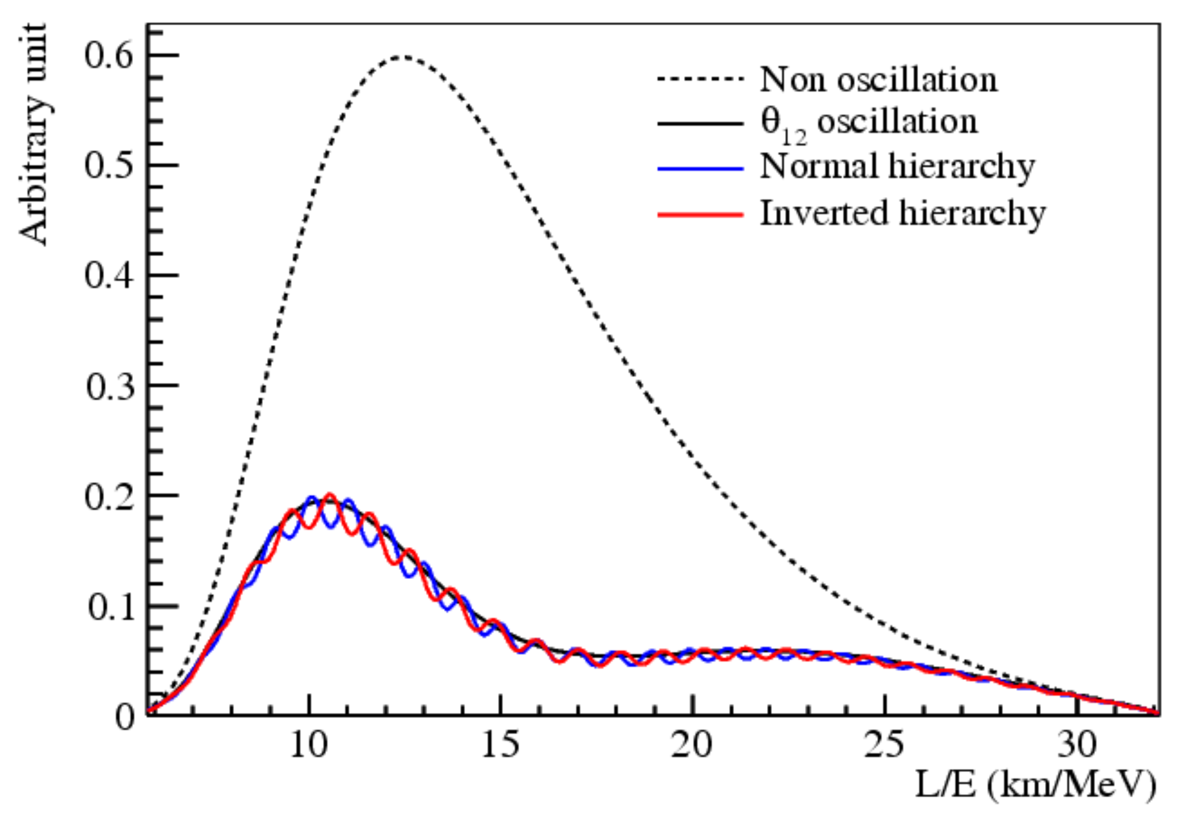
In order to discriminate between the two possible hierarchies, we need to determine the energy spectrum with a very high energy resolution. The experimental signature of the reactor is given by the inverse beta decay process . The resulting signal is given by visible energy from the positron energy loss and annihilation, plus delayed light, at a fixed 2.2 MeV energy, from the neutron capture on protons.
Figure 2 shows the spectrum in the non-oscillating case (dashed line) and the expected spectrum for a detector with a baseline of about 50 km, as in the JUNO experiment case. The hierarchy-dependent corrections are in phase opposition—the blue line represents the NH and the red line the IH.
2. JUNO Detector and Capabilities
The JUNO (Jiangmen Underground Neutrino Observatory) detector will be built at a shallow depth, with an average overburden of about 700 m, close to Jiangmen City, China, at a 53 km distance from the Yangjiang and Taishan nuclear power plants. The foreseen total power produced by the two facilities is about 26.6 GW.
The core of the detector is composed of 20 kton of liquid scintillator (LS), contained in an acrylic sphere (12 cm thick, with an inner diameter of 35.4 m), kept in position by a stainless steel truss. This central detector is placed inside an active water pool that will act as a Cherenkov muon veto and will reduce gamma rays and neutrons coming from the rock. On top of the water pool there will be an external veto detector composed of plastic scintillators.
The LS is composed of LAB (linear alkyl benzene) as solvent, with PPO (2.5-diphenyloxazole) as fluor and bis-MSB, a wavelength shifter.
In order to attain the desired energy resolution to disentangle the two mass hierarchies, the JUNO Collaboration paid particular attention to the photomultiplier system, which consists of 17,000 large PMTs, with a diameter of 20 inches, interspersed with 25,000 smaller ones of 3 inch diameter. This large number of PMTs will allow powerful event reconstruction and will offer an internal cross-check, which should help in reducing the non-stochastic uncertainty and improving the high-precision oscillation parameter measurement. The total coverage is about , corresponding to about 1200 photo-electrons/MeV.
To analyze the spectrum, distinguish the position of variation in the flux oscillation, and extract the desired mass hierarchy information, the total energy resolution must be .
3. Mass Hierarchy and Neutrino Physics
The main goal of JUNO is to establish the neutrino mass hierarchy by analyzing the spectrum of the antineutrino inverse decay on proton. To obtain this result, the experimental spectrum will be compared with the theoretical one, which is a function of the oscillation parameters and of the mass hierarchy.
This discrimination is obtained by comparing the values corresponding to the two different hierarchies’ best fit points.
The term is a measure of the mass hierarchy sensitivity, and represents the discrimination power of JUNO [2].
In addition to the mass hierarchy determination, JUNO will perform other measurements and analyses. Thanks to the very high statistics and the excellent energy resolution JUNO will provide a significant improvement in the precision measurement of the three masses and mixing parameters (see Table 1) [3].
4. Neutrino Astrophysics
4.1. Supernova Neutrinos
The rich JUNO programme also covers neutrino astrophysics. A supernova (SN) explosion causes the emission of a huge amount of energy in the form of neutrinos over a long time period. JUNO can perform studies of supernovae, both with the direct measurement of the neutrino burst produced by a nearby SN collapse and with the study of the diffuse supernova background (DSNB).
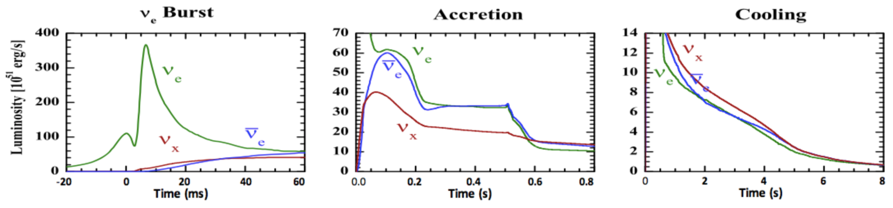
Analyzing the three different stages in which the SN explosion process can be divided (i.e., the very fast initial neutrino burst, the accretion phase, and the cooling phase), it is possible to infer many parameters of interest for astrophysics and for elementary particle physics (see Figure 3).
These three phases have different emission spectra, and thanks to this difference it is possible to obtain complementary information on the neutrino (antineutrino) flavor composition and luminosity and to probe SN models in term of time evolution, energy spectra, and flavor mixing.
Table 2 lists the main interaction channels and the number of expected events in JUNO, for a 10 kpc distant SN.
4.2. Solar Neutrinos
Solar neutrinos can also be studied with the JUNO detector. Despite the shallow site, the JUNO detector takes advantage of its large LS mass (which guarantees a very high statistics), and of its very good energy resolution.
For these studies, a key parameter is the radiopurity level of the LS, in order to disentangle the signal from the different natural background sources. In particular, the radioactive isotopes , , , , and must be considered. Table 3 shows the background rate constraints required to conduct low-energy solar neutrino measurements, as well as the estimated solar neutrino signal rates at JUNO.
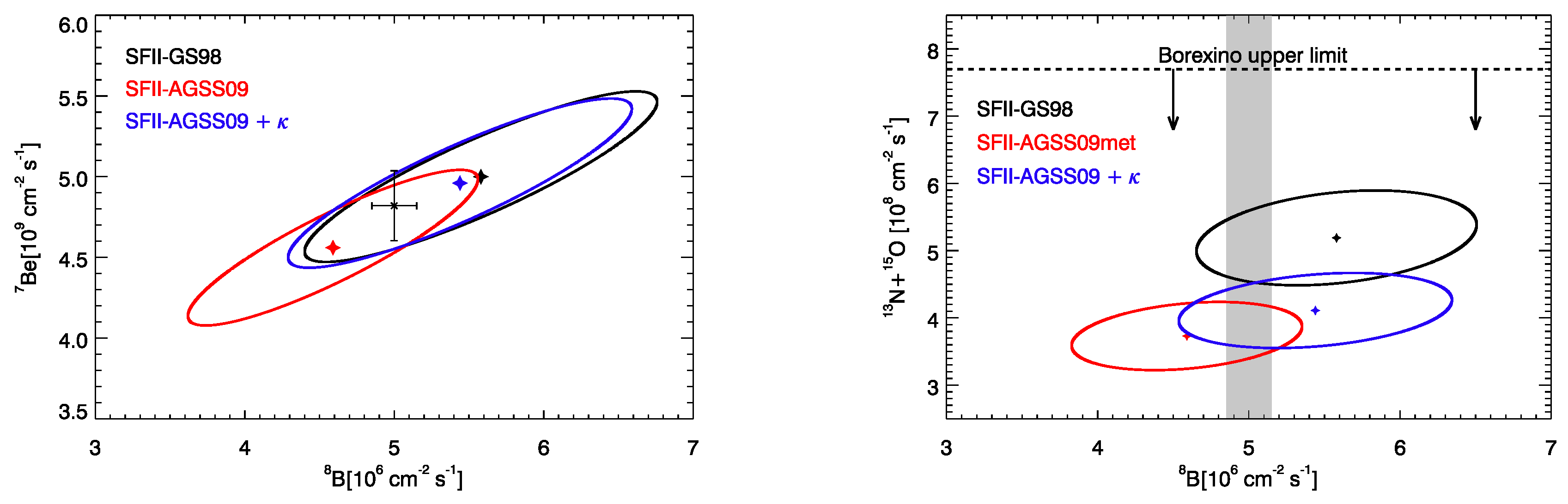
One of the major concerns in solar neutrino physics is the so called “solar metallicity problem” (SMP), about the content of metals in the core of the Sun [6]. These different possible versions of low Z vs. high Z of the standard solar model affects the neutrino fluxes. An improvement in the accuracy of the determination of the flux for Be and for B could help in solving the SMP.
As shown in the left panel of Figure 4, the experimental results were compatible with the predictions for both the low Z and high Z models. This means that it is not possible to definitely solve this ambiguity only by looking at Be and B fluxes. A breakthrough would come with the measurement of the CNO neutrino fluxes, as shown in the right panel of Figure 4. This graph also indicates that a parallel improvement in the determination of one of the two fluxes, measurable with the JUNO detector, would bring a complementary piece of information, essential to discriminate the ambiguity between high-Z models and models predicting low Z metallicity with modified opacity.
The possibility of observing B neutrinos is guaranteed in an experiment characterized by a high photon yield, like JUNO, with a relatively low threshold and very good energy resolution. The main problem is due to the cosmogenic background of long-lived spallation radioisotopes. The most troublesome for the elastic scattering channel are Li, N, and particularly the Be, whose spectra cover almost all the energy regions of interest and decay slowly (≫1 s).
Besides the standard elastic scattering, another channel for the B neutrino study is the charged current interaction, mainly with with an energy threshold of 2.2 MeV.
Another open issue in solar neutrino physics is the study of the transition region between the low-energy vacuum oscillation and the higher energies, where the MSW mechanism dominates. It is important to test the stability of the large mixing angle (LMA) oscillation solution, also considering additional contributions to the “standard” oscillation pattern, due, for instance, to non-standard neutrino interactions (NSIs).
The high statistics and the excellent energy resolution of JUNO could perform a detailed study of the spectrum in the transition region around 3–4 MeV.
4.3. Geoneutrinos
Natural radioactivity within the Earth represents a powerful source of heat, influencing the thermal history of our planet. Radiogenic and primordial Earth heat constitute two of the main contributions to the total energy loss of the Earth. Available measurements of temperature gradients in mines gives a total thermal production of 46 ± 3 TW [8].
Measuring the emitted in the and radioactive decay chains (geoneutrinos) and testing the rate helps in understanding the abundance of radioactive elements and, therefore, the radiogenic heat contribution and by extension the Earth’s composition (e.g., Ref. [9]).
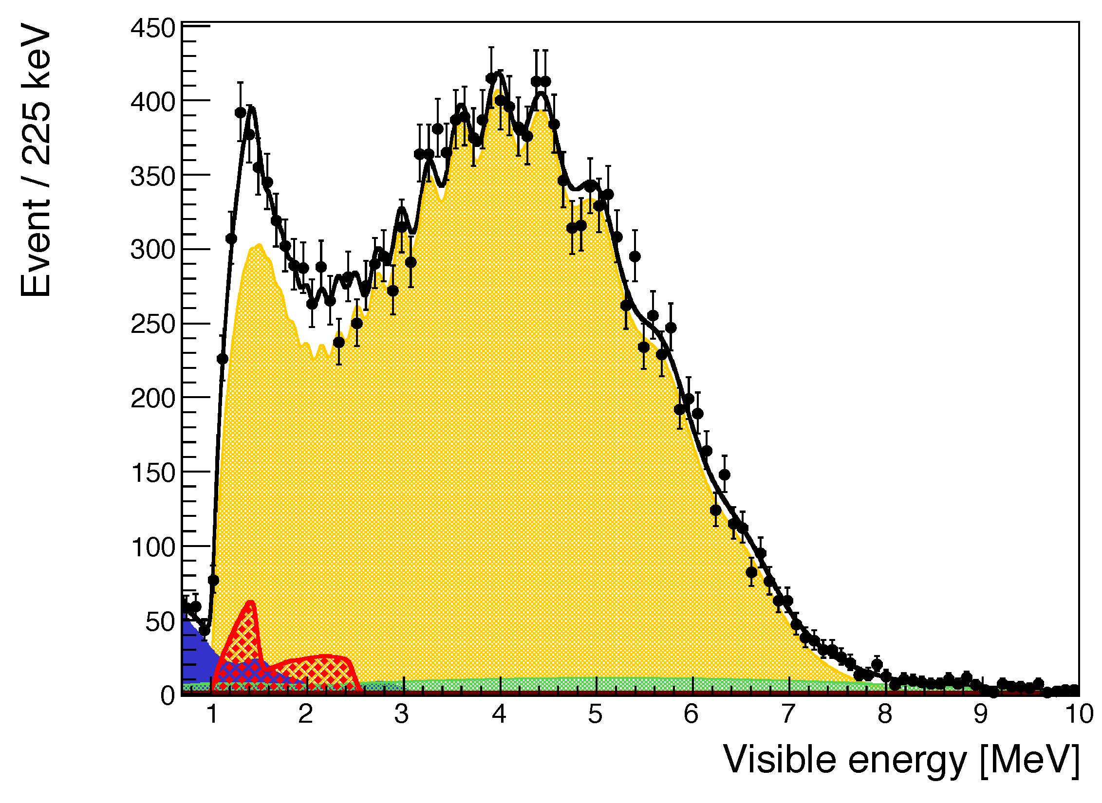
The potential of the JUNO detector for geoneutrino measurements is due to its depth and radiopurity and, in particular, to its huge size. The main difficulty comes from the presence of a very significant background, with respect to the analyzed signal of inverse decay, due to reactor antineutrinos, as shown in Figure 5, where the expected geoneutrino signal is represented in red.
Despite the large reactor antineutrino contribution, one expects an important geoneutrino measurement at JUNO, which already in the first year of data collection should detect between 300 and 500 events, which is more than the number of geoneutrinos detected by that time by all the other available experiments (KamLAND, Borexino, and SNO+).
5. Conclusions
The JUNO detector, with an unprecedented size, PMT coverage, light yield, and energy resolution, has a high potential to determine the neutrino mass hierarchy, using neutrino oscillations in vacuum. It is rapidly progressing through the design, prototyping, and construction phases, and besides its main physics goal, it will also be able to precisely measure the neutrino oscillation parameters below the 1% level, pursuing a rich neutrino physics and astrophysics programme. The experiment is scheduled to start data collection in 2021.
Funding
This research received no external funding.
Conflicts of Interest
The authors declare no conflict of interest.
References
- Qian, X.; Vogel, P. Neutrino mass hierarchy. Prog. Part. Nucl. Phys. 2015, 83, 1–30. [Google Scholar] [CrossRef] [Green Version]
- An, F.; An, G.; An, Q.; Antonelli, V.; Baussan, E.; Beacom, J.; Bezrukov, L.; Blyth, S.; Brugnera, R.; Avanzini, M.B.; et al. Neutrino Physics with JUNO. J. Phys. G 2016, 43, 030401. [Google Scholar] [CrossRef]
- Esteban, I.; Gonzalez-Garcia, M.C.; Maltoni, M.; Martinez-Soler, I.; Schwetz, T. Updated fit to three neutrino mixing: Exploring the accelerator-reactor complementarity. J. High Energy Phys. 2017, 2017, 87. [Google Scholar] [CrossRef]
- Choubey, S.; Petcov, S.T.; Piai, M. Precision neutrino oscillation physics with an intermediate baseline reactor neutrino experiment. Phys. Rev. D 2003, 68, 113006. [Google Scholar] [CrossRef]
- Lodovico, F.D. The State of the Art of Neutrino Physics; World Scientific: Singapore, 2018; pp. 261–297. [Google Scholar]
- Antonelli, V.; Miramonti, L.; Pena Garay, C.; Serenelli, A. Solar Neutrinos. Adv. High Energy Phys. 2013, 2013, 351926. [Google Scholar] [CrossRef]
- Serenelli, A.M. A Special Borexino Event—Borexino Mini-Workshop—2014. September 2014. Available online: http://borex.lngs.infn.it/ (accessed on 11 November 2018).
- Davies, J.H.; Davies, D.R. Earth’s surface heat flux. Solid Earth 2010, 1, 5–24. [Google Scholar] [CrossRef]
- Bellini, G.; Ianni, A.; Ludhova, L.; Mantovani, F.; McDonough, W.F. Geo-neutrinos. Prog. Part. Nucl. Phys. 2013, 73, 1–34. [Google Scholar] [CrossRef] [Green Version]
| 1 | The first result is obtained mainly from solar neutrino and from KamLAND experiments. The second result is obtained mainly from atmospheric and by long baseline accelerator experiments. This second value would correspond to in the case of inverted hierarchy. |
| 2 | with P’s weights as 40:2:1. |
| 3 | For details of the calculation see Ref. [2]. |
Figure 1.
Neutrino mass eigenstate flavor composition and mass pattern in the two cases of normal (left) and inverted (right) hierarchies. Taken from Ref. [2].
Figure 1.
Neutrino mass eigenstate flavor composition and mass pattern in the two cases of normal (left) and inverted (right) hierarchies. Taken from Ref. [2].

Figure 2.
The relative shape difference of the reactor antineutrino flux for different neutrino mass hierarchies (MHs) [2]. The figure represents the product of the neutrino flux times the interaction cross section times the survival probability.
Figure 2.
The relative shape difference of the reactor antineutrino flux for different neutrino mass hierarchies (MHs) [2]. The figure represents the product of the neutrino flux times the interaction cross section times the survival probability.

Figure 3.
Three phases of neutrino emission from a core-collapse supernova (SN), from left to right: (left) Infall, bounce, and initial shock-wave propagation, including prompt burst. (middle) Accretion phase with significant flavor differences of fluxes and spectra and time variations of the signal. (right) Cooling of the newly formed neutron star, with only small flavor differences between fluxes and spectra. collectively stands for neutrinos and antineutrinos of all three flavors. Figure from Ref. [2].

Figure 4.
Theoretical predictions and experimental results for solar fluxes. The flux is reported on the x-axis. On the vertical axis, instead, one can see the fluxes of (left) and of + , from CNO cycle (right). The experimental results correspond to black bars in the left graph and to shaded gray vertical band in the right one. The theoretical allowed regions in high Z, low Z, and low Z with modified opacity versions of the standard solar model (SSM) correspond, respectively, to black, red, and blue ellipses. Taken from Ref. [7].

Figure 5.
Monte Carlo estimate of the prompt IBD candidates for 1 year of measurements, with fixed chondritic Th/U mass ratio. The expected geo- signal is represented in red, and other components are: the reactor antineutrinos (orange), main background component, (green), accidental (blue). From Ref. [2].


Table 1.
Comparison of the present accuracy and the JUNO (Jiangmen Underground Neutrino Observatory) potentialities for three oscillation parameters.
Table 1.
Comparison of the present accuracy and the JUNO (Jiangmen Underground Neutrino Observatory) potentialities for three oscillation parameters.
| Oscillation Parameter | Current Accuracy | Dominant Experiment (s) | JUNO Potentialities |
|---|---|---|---|
| (Global ) | |||
| KamLAND | |||
| MINOS, T2K | |||
| SNO |
Table 2.
Expected number of events in JUNO for the main channels for neutrinos produced by a SN at a distance of 10 kpc. Taken from Ref. [2].
Table 2.
Expected number of events in JUNO for the main channels for neutrinos produced by a SN at a distance of 10 kpc. Taken from Ref. [2].
| Process | Type | Events |
|---|---|---|
| 〈E〉 = 14 MeV | ||
| + p → e + n | CC | 5.0 × 10 |
| NC | ||
| ES | ||
| NC | ||
| CC | ||
| CC |
Table 3.
The requirements of singles background rates for conducting low-energy solar neutrino measurements and the estimated solar neutrino signal rates at JUNO. Taken from Ref. [2].
Table 3.
The requirements of singles background rates for conducting low-energy solar neutrino measurements and the estimated solar neutrino signal rates at JUNO. Taken from Ref. [2].
| Internal Radiopurity Requirements | ||
|---|---|---|
| Baseline | Ideal | |
| Pb | (g/g) | (g/g) |
| Kr | 500 (counts/day/kton) | 100 (counts/day/kton) |
| U | (g/g) | (g/g) |
| Th | (g/g) | (g/g) |
| K | (g/g) | (g/g) |
| C | (g/g) | (g/g) |
| Cosmogenic Background Rates (counts/day/kton) | ||
| C | 1860 | |
| C | 35 | |
| Solar Neutrino Signal Rates (counts/day/kton) | ||
| pp | 1378 | |
| Be | 517 | |
| pep | 28 | |
| B | ||
| N/O/F | ||
© 2018 by the authors. Licensee MDPI, Basel, Switzerland. This article is an open access article distributed under the terms and conditions of the Creative Commons Attribution (CC BY) license (http://creativecommons.org/licenses/by/4.0/).
Share and Cite
MDPI and ACS Style
Miramonti, L. Neutrino Physics and Astrophysics with the JUNO Detector. Universe 2018, 4, 126. https://doi.org/10.3390/universe4110126
AMA Style
Miramonti L. Neutrino Physics and Astrophysics with the JUNO Detector. Universe. 2018; 4(11):126. https://doi.org/10.3390/universe4110126
Chicago/Turabian StyleMiramonti, Lino. 2018. "Neutrino Physics and Astrophysics with the JUNO Detector" Universe 4, no. 11: 126. https://doi.org/10.3390/universe4110126
Note that from the first issue of 2016, this journal uses article numbers instead of page numbers. See further details here.