1. Introduction
Hydrologic predictability depends on knowledge of initial hydrologic conditions. While current precipitation may be the most visible hydrological driver of streamflow, antecedent states of groundwater and soil moisture are less visible, but of critical importance. These conditions serve as major factors in runoff generation and are fundamental obstacles in the accurate prediction of river discharge [
1,
2,
3,
4,
5]. Traditionally, the analysis and prediction of hydrologic extremes have involved statistical assessments of long-term (30+ years) climatic and hydrological datasets to determine flood thresholds, severity, and recurrence intervals. Contemporary extremes analysis and monitoring has not deviated much from its roots, however past events are not always indicative of future conditions, especially under current climatic trends [
6]. Efforts to improve hydrological prediction and reduce uncertainty can now leverage a wealth of new tools for measurement and estimation of land surface states, namely satellite remote sensing products and advanced numerical models [
7].
The joint NASA/DLR Gravity Recovery and Climate Experiment (GRACE) satellite mission [
8] has been an important step forward in observing terrestrial water storage with global coverage. GRACE provides monthly data on changes in the Earth’s gravity field, which we assume to be correlated with the movement of water through the Earth’s system at specific temporal and spatial scales. GRACE has been providing monthly gravity field solutions since April 2002, and has proved an effective tool to observe changes in the mass of ice sheets [
9], snow mass [
10], groundwater storage [
11,
12,
13], surface water storage [
14], and to hydrologic drought characterization [
15,
16,
17].
GRACE has also contributed to flood analysis [
18,
19]. Generally, the land surface modulates the connection between precipitation and runoff generation through two basic mechanisms: infiltration limitation and saturation excess. During floods, one of these two mechanisms is typically identified as a driver based on the pre-flood conditions and the nature of the precipitation event. However it is difficult to ascertain the relative contribution of each. For example, preceding flood occurrence, water tables can gradually rise, saturating soils at depth and creating a dangerous precondition for sudden intense runoff generation. Though it has been a primary research topic in hydrology for years, three recent research papers have explored non-linearities in the relationship between river discharge and basin-averaged water storage using GRACE observations [
19,
20,
21]. The idea that extreme values in terrestrial water storage have the ability to augment runoff generation during future flood events at several months lead-time has been previously referred to as “flood potential” [
18]. This is distinctly different from river flood prediction, as streamflow forecasting is not employed. However, the monitoring of flood potential could provide valuable anticipatory capacity for water/natural resource managers.
GRACE terrestrial water storage anomaly (TWSA) data can contribute to an improved understanding of soil moisture and groundwater contributions to future runoff generation, but the utility of GRACE data for operational analysis or actionable prediction is challenging. Three prevailing limitations are: (1) coarse spatial resolution (one arc-degree for the level-three data product [
22]); (2) the aggregated observation of multiple water storage components (
i.e., snow, soil moisture, and groundwater) as a single integrated value for each grid cell; and (3) latency in data product processing and release (2–4 months lag) [
23]. These obstacles make many applications difficult, as water resource management tends to occur at watershed scales and on daily to weekly timescales.
Computer modeling of land surface processes offers the potential for a level of temporal and spatial coverage beyond the capacities of most
in situ observation networks. However, land surface model simulation accuracy suffers from the assumptions and simplifications that accompany an empirical representation of reality [
24]. Even though many land surface models (LSMs) include detailed descriptions of vegetation and soil moisture parameters, the interactions between deeper, subsurface (
i.e., groundwater) and surface water, and the accurate generation of lateral surface and subsurface flows are typically disregarded. This can cause models to have predictive inaccuracies in situations where subsurface contributions to streamflow generation are important [
25].
Data assimilation is the process of merging measurements with model predictions to maximize spatial and temporal coverage, consistency, resolution, and accuracy. It addresses weaknesses in the representation of land-surface model states at the grid scale level, and can create more realistic predictions of hydrological components like runoff, river flow, and groundwater [
26,
27]. In hydrology, data assimilation is often assumed to be an improvement over raw observations or a model without assimilation, such that the assimilation adds unique information from both sources in order to achieve a better combined product.
The assimilation of GRACE terrestrial water storage observations has been shown to improve model outputs in several cases, decreasing RMS errors, and increasing the correlation between simulated and observed variables. Zaitchik
et al. [
28] discusses several potential advantages of GRACE data assimilation. For example, the pairing of GRACE estimates with a watershed-defined Catchment Land Surface Model (CLSM) domain allows for area-accurate assimilation within hydrologically-defined basins. Unlike many land surface models, CLSM provides a representation of surface and subsurface hydrologic states, including groundwater, which can be applied directly as an equivalent state variable to the integrated GRACE observations (TWSA). Additionally, the spatial resolution of modeled segments provide a physically-based mechanism for distributing GRACE observations at spatial scales smaller than the native resolution. Houborg
et al. [
15] suggest that data assimilation may be the key to realizing the full potential of intrinsically-coarse GRACE TWSA observations. The outcomes of these studies included moderate, but statistically significant, improvements to the hydrological modeling skill of the CLSM across major parts of the United States. Li
et al. [
16] also recognized the potential for GRACE data to improve the simulation of land surface processes for drought monitoring applications.
In May and June of 2011, a large flood crest moved down the Mississippi from a combination of snowmelt and heavy spring rains in the Missouri river basin. Streamflow in the Missouri were characterized as a 500-year event. Red River Landing, near the mouth of the Mississippi, went above flood stage on 19 March and did not fall below flood stage until 25 June [
29].
We build upon previous work [
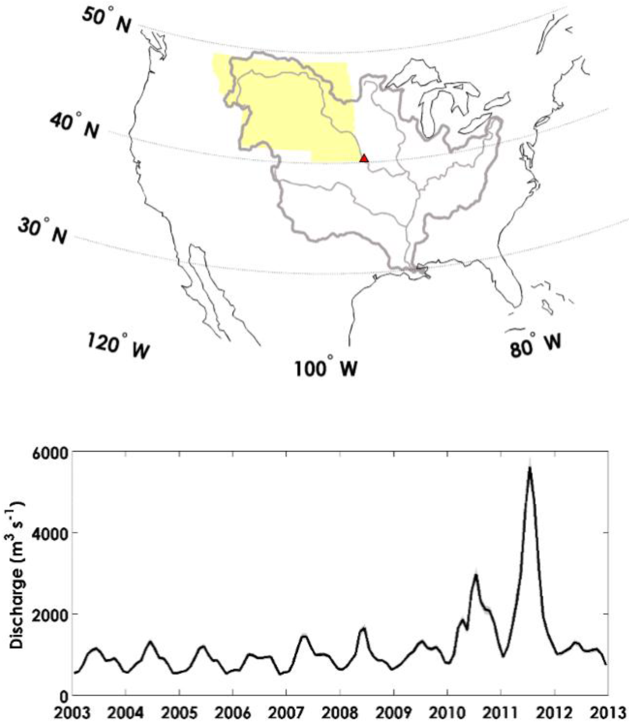
19] that demonstrated record-length maxima in GRACE TWSA over the Missouri river basin during the months of June and July 2011 coincident with peak stream flow. This basin contributed intense snowmelt and groundwater discharge to the high river levels preceding the storm events of March–July 2011. We apply the National Climate Assessment “Northern Plains” domain to isolate the study region of the Missouri River basin (
Figure 1). This entire region drains through a single point in the Missouri river and, as such, is suitable to constrain the water balance there. Following the river gage selection procedure described in Reager
et al. [
19], we use USGS stream gage #6818000 at St. Joseph, Missouri (
Figure 1).
Figure 1.
Study domain, stream gage near the mouth of the Missouri river, and monthly flow time series.
Figure 1.
Study domain, stream gage near the mouth of the Missouri river, and monthly flow time series.
Here we examine disaggregated water storage outputs from the GRACE-assimilated CLSM (CLSM-DA) to explore the utility of GRACE assimilation for the characterization of long lead-time river basin flood potential for an exceptional event in the Mississippi river basin. We determine the effects of assimilation by exploring disparities between CLSM-DA outputs, GRACE observations, and CLSM Open-Loop runs (CLSM-OL; obtained by running the CLSM without any data assimilation). We evaluate the improvement in the model state prediction by validation with groundwater well observations.
To provide a brief overview of the organization of the paper: In
Section 2, we present results on the model validation, on the disaggregation of the water storage components, on the spatial distribution of water storage components before and during flooding, and on the contributions of water storage components to event generation. In
Section 2.5 we discuss the implications of the results.
Section 3 is the experimental section, and contains detailed information on the experiment setup, on the CLSM model structure, and on the assimilation methodology.
2. Results
2.1. Validation and Performance Assessment
USGS well observations were utilized for 16 monitoring well locations through the study domain (
Figure 2). Well locations were chosen based on length and completeness of record, and for a geographical representation across the entire study area. Well data were processed by removing their 2003–2014 record-length mean water table depth (from 12 to 65 feet in shallow unconfined aquifers), removing the record-length seasonal climatology and then normalizing each well time series by its record-length standard deviation. This results in 14 time series of well variability that can be averaged to generate a single regional time series. USGS well stations used are: 480034105195404; 483127103373102; 472203111112602; 46540100222101; 463417099271002; 450524112380701; 473051099093601; 430027102311806; 420757104024701; 434329096521201; 420757104024701; 423730098560001; 423148098300601; 400155101521302; 392045093302401; and 383644091124901.
Figure 2.
USGS well observation locations and normalized time series (grey lines), as well as the average of the normalized time series (red line).
Figure 2.
USGS well observation locations and normalized time series (grey lines), as well as the average of the normalized time series (red line).
The aggregated well time-series was then compared to the model groundwater estimates for the domain under the same processing. While this does not allow for evaluation of a realistic water table, the model representation of groundwater storage is empirical and is best evaluated for its relative variability and timing as opposed to absolute accuracy.
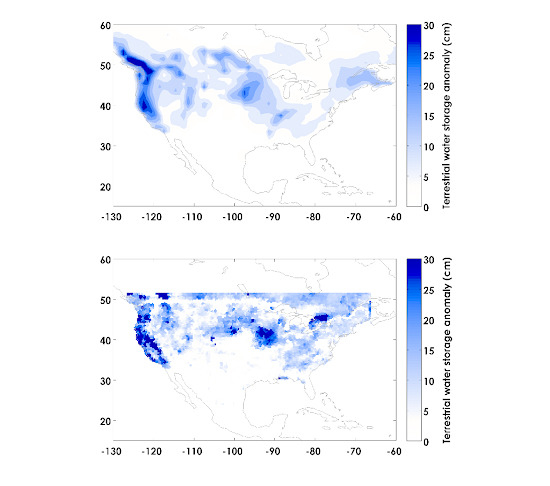
Figure 3 shows maps of GRACE observations and model outputs for March 2011, the month of highest snow melt and high water storage loading preceding flood initiation in May 2011 [
19]. The bottom right panel shows the difference in terrestrial water storage before and after assimilation in the model for that month. In the assimilated model, there are generally wetter antecedent conditions in the study watershed several months prior to the spring floods. In this month, GRACE increases the model domain water storage by roughly 40 km
3, or an average of 0.5 cm equivalent.
Figure 3.
Pre-flood terrestrial water storage anomaly in March 2011: (a) GRACE observations; (b) CLSM open-loop simulation; (c) CLSM-DA assimilation simulation; (d) the difference between the two model simulations, CLSM-DA minus CLSM.
Figure 3.
Pre-flood terrestrial water storage anomaly in March 2011: (a) GRACE observations; (b) CLSM open-loop simulation; (c) CLSM-DA assimilation simulation; (d) the difference between the two model simulations, CLSM-DA minus CLSM.
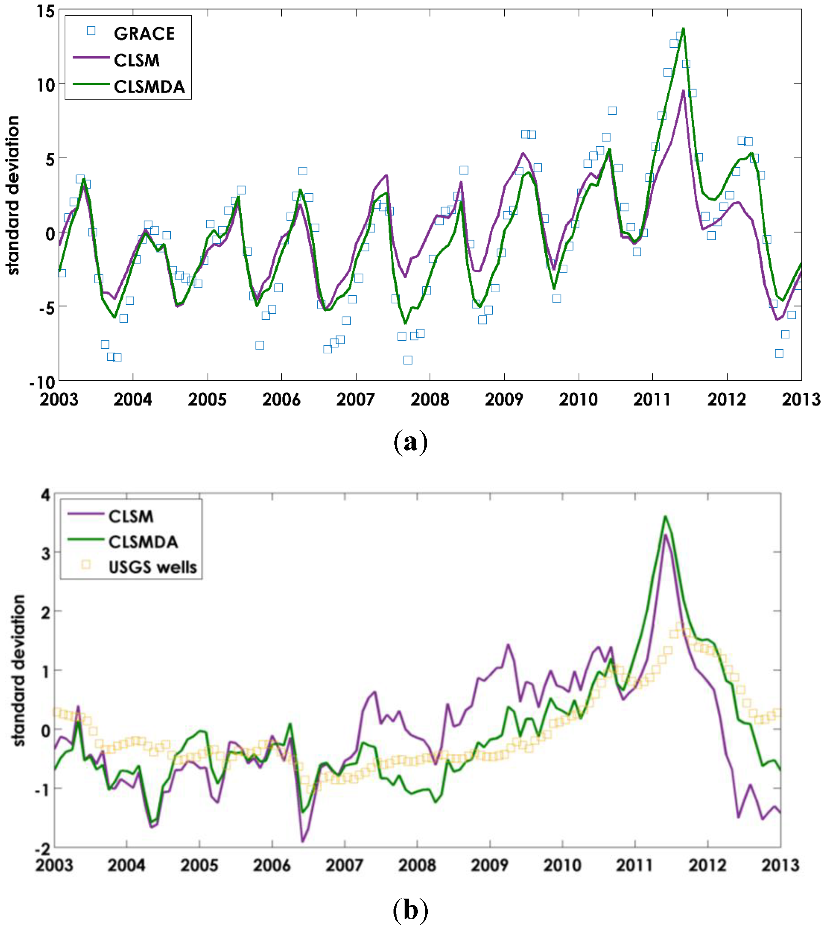
Figure 4a shows the comparison of the region-averaged GRACE time-series with two model outputs after normalization. We see that the CLSM-DA run matches the GRACE observations more closely than the open-loop (CLSM).
Figure 4b shows the comparison of model groundwater storage anomaly (
i.e., not total water storage) with the USGS well observations after removal of the record-length climatology and normalization. The monthly climatology was removed from each of the time series to demonstrate the inter-annual persistence of above- and below-normal storage anomalies.
Table 1 contains the summary statistics for the two comparisons.
Figure 4.
(a) The effect of assimilation on Terrestrial Water Storage in the Northern Plains domain, showing the region-averaged GRACE TWSA, the open-loop model (CLSM), and the GRACE-assimilated model (CLSMDA); (b) well validation for the Northern Plains region, showing the groundwater component only from the open-loop model (CLSM), the GRACE-assimilated model (CLMSDA), and independent well observations averaged over the region (climatology removed in each).
Table 1.
Goodness of fit statistics for assimilation effects and validation of assimilation improvement of domain-averaged groundwater state estimation with well observations. All statistics are significant at the 95% confidence level.
Table 1.
Goodness of fit statistics for assimilation effects and validation of assimilation improvement of domain-averaged groundwater state estimation with well observations. All statistics are significant at the 95% confidence level.
| Model | Metric | GRACE TWSA | USGS Groundwater Anomaly |
|---|
| CLSM Open-Loop | r | 0.88 | 0.58 |
| RMSE | 33 cm | 2.32 (normalized) |
| CLSM DA | r | 0.95 | 0.86 |
| RMSE | 25 cm | 1.81 (normalized) |
2.2. Vertical Disaggregation
Figure 5 shows the vertically disaggregated components of the residual CLSM-DA time series (TWS, groundwater, RZMC, SFMC, and SWE) and GRACE residual TWSA (gold squares), for the Northern Plains region. The seasonal climatology of each time series has been removed in order to isolate inter-annual variability. Overall, CLSM-DA TWSA deficits are comparable to those from GRACE, though several events are underestimated in the study area.
The plots reveal timing differences between changes in water stores. For example, there are occasions where RZMC residuals lead groundwater changes by one to three months. RZMC also shows the most monthly variation between positive and negative values out of the storage components (i.e., as a small reservoir, it dries and wets quickly). In the Northern Plains, RZMC recovers for one to two months on several occasions during extended deficit periods while the other stores remained negative. Peak SWE residuals were often matched or immediately followed by an instance of surplus RZMC, as snow melt filled the root-zone.
For the 2011 flood event, CLSM-DA storage beneath the soil layer (
i.e., “groundwater”) was a large portion of the signal before flood occurrence. Post event flood reports [
19] showed that in the Missouri River basin (represented here as the Northern Plains study area), the groundwater storage climbed to record levels, accompanied by record high snow water equivalent a few months before. It is likely that record snowmelt and a high water table contributed to flooding in this event [
19], and that mechanism seems consistent with the assimilation results.
Figure 5.
CLSM-DA disaggregated, residual terrestrial water storage time series (i.e., climatology removed) for the Northern Plains region. Time period is from January 2003–April 2014. Negative values designate deficits and positive surplus. Variables on the left axis are: CLSM-DA total water storage (green shading), Below RZMC or “groundwater” (black), RZMC (green), and monthly GRACE TWSA (gold squares). Variables on the right axis are: CLSM-DA SFMC (red dashed) and SWE (blue dashed). Units are centimeters of equivalent water storage.
The structure of the CLSM model is such that a terrestrial water storage variable is estimated and assumed to contain snow water equivalent, soil moisture, and some residual value of subsurface water (see
Section 3.2). This residual value is then assumed to be “groundwater” though, realistically, for regions with large or dynamic surface water, the residual term would also include those components, especially in the case that they are highly correlated, temporally.
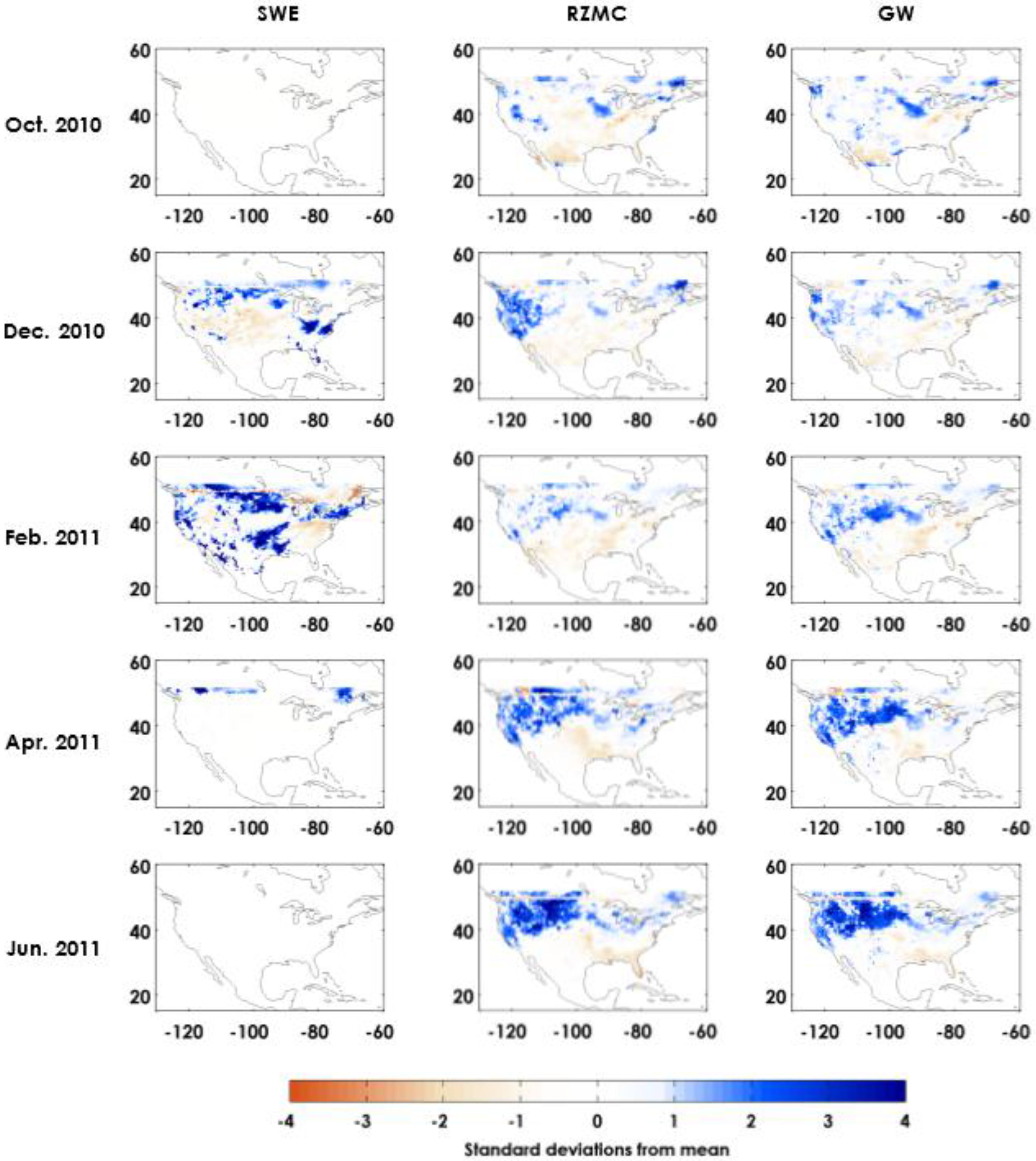
2.3. Spatially Distributed View of Event Progression
Figure 6 shows the event progression for the Northern Plains floods in a series of maps for each state variable. The colors depict the number of standard deviations each grid cell is away from its record-length mean value. As could be determined from the time series, SWE achieves a record maximum in the months preceding the 2011 floods in the Missouri basin region. There are SWE values in the domain of more than 4-sigma for the month of February. This indicates the non-Gaussian nature of the time series, and that solid water storage was considerably higher than normal. Snow in the Missouri basin was reported as a record high in the months preceding the flood [
29].
Groundwater and soil moisture both increase substantially and rapidly during the months after snowmelt preceding flood occurrence (April 2011). It is these two variables that indicate regions of enhanced flood potential. Visually, these two variables are highly correlated in space and time, which may be due to model structural limitations as much as it is to any physical mechanism.
Figure 6.
Time progression of the 2011 flood event, showing (left) snow water equivalent; (middle) root-zone soil moisture; and (right) groundwater from the CLSMDA simulation for October 2010 through June 2011.
Figure 6.
Time progression of the 2011 flood event, showing (left) snow water equivalent; (middle) root-zone soil moisture; and (right) groundwater from the CLSMDA simulation for October 2010 through June 2011.
2.4. Contributions to Event Generation
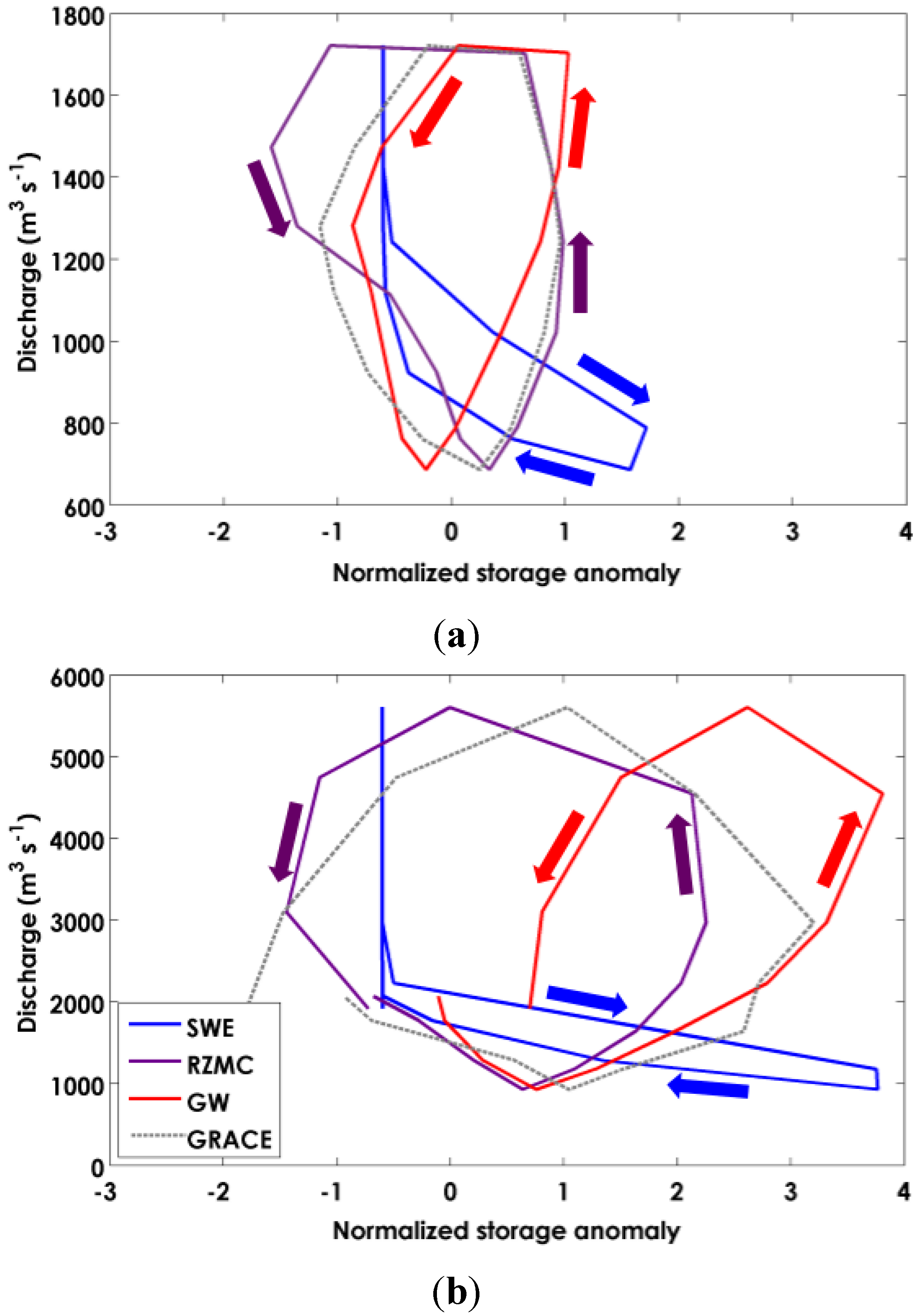
Figure 7 shows the hysteresis between CLSMDA state variables and streamflow at the USGS gage. Following Sproles
et al. [
21], we use these relationships to understand the dynamics of the basin and how individual state variables affect a discharge response. In a normal (average) year (
Figure 7a), there is nearly an equivalent curvature between soil-streamflow hysteresis and groundwater-streamflow hysteresis.
Figure 7.
Hystereses between stream flow at the mouth and snow water equivalent (SWE), root-zone soil moisture (RZMC), or groundwater (GW) in the CLSMDA during (a) the climatological average of all years; and (b) the 2011 flood year. Raw GRACE data are shown for comparison. Hystereses run from October to September.
During the flood year, all hysteresis loops expand along both axis due to increased storage in all state variables (horizontal) and increased discharge (vertical). However, the groundwater and snow hysteresis loops separates horizontally, demonstrating exceptional storage in the months preceding flood occurrence. This heavy skewing in the positive-storage direction shows the extent of the positive anomaly in groundwater preceding flood (nearly four standard deviations), and supports the hypothesis of groundwater as a major contributor to event generation.
2.5. Discussion
A comparison of hydrologic variables from direct observation, CLSM data-assimilated outputs, and CLSM Open-Loop runs was conducted to evaluate the accuracy and utilization of CLSM-DA for flood potential analysis. Data assimilation provides spatial resolutions currently unattainable with GRACE alone. Correlation results show that data assimilation improved CLSM TWSA simulations in the study region. CLSM-DA is a viable dataset for hydrologic analyses based on several potential benefits. This analysis suggests a useful tool for flood potential assessment—one that identifies and quantifies terrestrial water storage extremes with higher resolution (compared with GRACE alone), provides a separation of terrestrial storage components, and provides a physically-based means to obtain terrestrial water storage information beyond the latest GRACE data release.
Data assimilation improved CLSM groundwater anomaly correlations significantly with aggregated well data. The ability to represent groundwater variability in the open-loop model is limited (r = 0.58), as the model does not possess enough information from forcing and physics alone. In this case, the assimilation helps to improve model accuracy in groundwater simulation (r = 0.86). The difference in the before- and after-assimilation correlation coefficients is statistically significant at the 99.8th percentile.
Generally, storage observed by GRACE versus the CLSM includes more terrestrial features, such as surface reservoirs, stream flow, human impacts on the hydrologic system (e.g., dams, river divergences), and subsurface variations below the model’s maximum depth (i.e., below two meters). Assimilation corrects the CLSM towards GRACE but still does not address shortcomings in the model structure that could lead to a degradation of simulation accuracy without a constant constraint on accuracy (e.g., in a hydrologic forecasting application). Still, the model provides a means to generate physically-based information beyond the last assimilation time step that is presumably (based on these results) better than the open-loop model alone.
Coarse resolution makes it challenging to apply GRACE observations towards local water resource management. CLSM-DA maps improve upon this, allowing us to identify key areas being affected by flood or drought conditions. Additionally, maps of proceeding months or seasons can help identify antecedent conditions that can lead to event generation in subsequent periods. For the 2011 event, we see very high snow water equivalent (3–4 months preceding peak discharge) and soil moisture (2–3 months preceding peak discharge) that indicate the ability of this methodology to provide event early warning. Assuming assimilation were performed and then the model was run past the assimilation time step, this would certainly provide a means to generate near real-time early warning information for regional flood potential.
With vertical disaggregation from the CLSM, we were able to assess relationships between SWE, SFMC, RZMC, and groundwater. There is evidence of one-to-two month lags between storage surplus appearance in SWE, surface soils, and the groundwater layer, as water takes time to infiltrate into the subsurface. This result highlights the impact that snowmelt can have on the water table, leading to dangerous pre-conditioning for large flood event generation.
The large basin storage-discharge relationship is highly non-linear in the Missouri, and is similar to results found in other studies [
19,
20,
21]. The hysteresis relationship is dynamic, with discharge responding to changes in basin storage at monthly time steps. This behavior is different than the traditional assumption in hydrology of a “linear reservoir”, or a near-linear proportional relationship between storage changes and discharge changes. The results shown in
Figure 7 suggest that this may be especially true for the groundwater-discharge relationship: groundwater reaches extreme (3-sigma) values several months before flood occurrence, and the assimilated model seems to capture this behavior.
There may be several reasons for the existence of such strong hysteresis behavior. Riegger and Tourian [
20] propose that the hysteresis effect is singularly attributable to temperature (
i.e., the freeze-thaw process), which acts to load a basin with snow and frozen soils in the winter months, loading basin storage without an equivalent increase in discharge. Then, when the spring melt arrives, discharge accelerates exponentially until losses overcome inputs and storage begins to draw down. However, this explanation can be controlled for in some basins (as those authors demonstrate), resulting in a hypothetical linear relationship again between storage and discharge.
We would offer, based on the present evidence, that controlling for snow accumulation should only affect the rising limb of the hysteresis and does not really offer a full description of what is happening in basins like the Missouri, especially with respect to hysteresis in subsurface water storage. Snow and frozen soils melt fairly quickly in the Missouri, especially in the low elevation prairie (within ~3 months,
Figure 6), and freeze-thaw may not provide a full explanation for the temporal displacement seen between storage and discharge. These results instead suggest a mechanism by which the storage and discharge are decoupled from the typical baseflow-driven linear reservoir process. In that case, a non-linearity in storage and discharge variability may be attributable to variable water retention in deeper soils. These are interesting phenomena for future research.


 ,
, 


