Hierarchical Regularization of Building Boundaries in Noisy Aerial Laser Scanning and Photogrammetric Point Clouds

Abstract

Aerial laser scanning or photogrammetric point clouds are often noisy at building boundaries. In order to produce regularized polygons from such noisy point clouds, this study proposes a hierarchical regularization method for the boundary points. Beginning with detected planar structures from raw point clouds, two stages of regularization are employed. In the first stage, the boundary points of an individual plane are consolidated locally by shifting them along their refined normal vector to resist noise, and then grouped into piecewise smooth segments. In the second stage, global regularities among different segments from different planes are softly enforced through a labeling process, in which the same label represents parallel or orthogonal segments. This is formulated as a Markov random field and solved efficiently via graph cut. The performance of the proposed method is evaluated for extracting 2D footprints and 3D polygons of buildings in metropolitan area. The results reveal that the proposed method is superior to the state-of-art methods both qualitatively and quantitatively in compactness. The simplified polygons could fit the original boundary points with an average residuals of 0.2 m, and in the meantime reduce up to 90% complexities of the edges. The satisfactory performances of the proposed method show a promising potential for 3D reconstruction of polygonal models from noisy point clouds.

1. Introduction

With the rapid developments in aerial laser scanning (ALS) and aerial oblique photogrammetry, 3D point clouds have become the primary datasets used in large-scale urban reconstruction [1,2]. In particular, recent advances in structure from motion (SfM) [3] and multi-view stereo (MVS) [4] methods allow detailed coverage of urban scenes, and are particularly suitable for feature matching [5], bundle adjustment [6,7], and dense image matching (DIM) [8,9] in aerial oblique images.

However, as the usability of point clouds or derived triangular meshes is limited by the difficulties in manipulating and managing the datasets, 2D polygons and polygonal building models are still the industrial standard datasets for various applications [10,11], including visualization, spatial analysis, urban planning, and navigation [12,13,14,15]. Although the extraction of points on the exterior building boundaries is gracefully handled by a standard convex hull or alpha-shapes for non-convex boundaries, simplification and regularization of the noisy boundaries are still non-trivial tasks and well-established cartographic algorithms do not produce acceptable results when applied to point cloud datasets.

The inherent deficiencies of point clouds data, such as data anisotropy, insufficient sampling, and especially noise, make it challenging to retrieve compact 2D/3D polygons of buildings that have satisfactory geometric quality. For ALS data, which have high altimetric accuracy but relatively low point density [16], the initial boundary points of building plans are often jagged [17] and small structures are not well sampled. Meanwhile, DIM point clouds of aerial oblique images are generally inferior to those created from laser scanning in terms of noise level and the preservation of sharp features [9]. The forward intersected point clouds suffer from inaccurate positioning at the edge of building planes due to disparity discontinuities, and thus sharp features may degenerate at corners.

In the boundary simplification process, traditional edge collapse-based methods are likely to eliminate sharp features, whereas regularization methods that adopt the Manhattan rule based on the dominant orientation tend to be too strict in many real-world applications, leading to large distortions when applied to polygons with multiple orientations.

This paper consists of three major contributions, in order to overcome the above issues: (1) we allow the mutation of boundary points along their normal in the local stage in a least-square manner to resist noise; (2) we relax the hard Manhattan assumptions (either parallel or perpendicular to the dominant orientation) [1] by also considering fidelity terms. Unlike other modified Manhattan-based regularization methods which need to pre-define the number of resulting orientations [18] or difference angle threshold for compulsive orthogonality [19], the proposed method casts the problem as a Markov random field (MRF) and allows multiple and arbitrary orientations with mutual regularities in the same optimization; and (3) we propose a strategy to produce simplified polygons with inter-part regularity in 3D space.

In this study, we extend our preliminary conference paper [20] in the following four directions: (1) improving the local stage regularization algorithm, allowing it to handle the zigzag effect more efficiently; (2) taking regional level relationships into considerations to handle boundary regularities between different planes or buildings; (3) conducting additional experiments on relatively low-density ALS data for building footprint generalization; and (4) supplementing more quantitative comparison with other representative methods. The rest of this paper is organized as follows. Section 2 briefly reviews the existing research on boundary points simplification and regularization. In Section 3, the proposed method is described in detail. The performance of the proposed method is evaluated in two different application scenarios, both qualitatively and quantitatively in Section 4. Discussions are given in Section 5 and the conclusions are presented in Section 6.

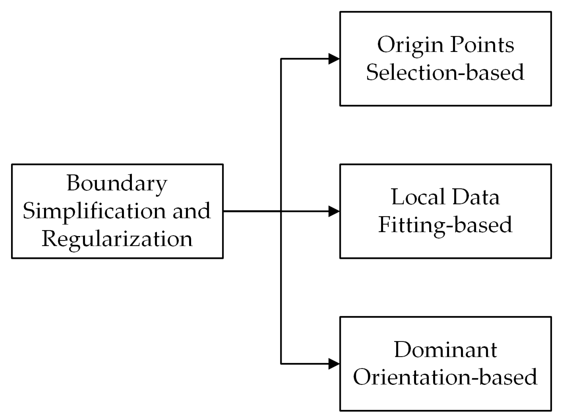
2. Related Work

The simplification and regularization of closed boundaries or polygons for discrete points have attracted a lot of interest in the fields of photogrammetry, cartography, and computer graphics. Such procedures can be used in map simplification [21], multi-scale representation [22,23], 3D model simplification [24], building footprint generalization [25], and 3D reconstruction [26]. However, the data redundancy and noise level in building borders from ALS or photogrammetric point clouds are distinctively higher than those in digital maps, existing building footprints, or 3D models. As shown in Figure 1, generally, producing methods for building boundary simplification and regularization can be categorized into three major classes.

The aim of boundary point simplification is to represent an original boundary compactly, which is necessary for efficient computation and visualization. The first class of methods attempted to decrease the number of vertices by discarding original points that met a certain criterion, locally or globally. Among this class of methods, the Douglas–Peucker algorithm, which uses perpendicular distance as a global indicator, is the most common [27]. Some algorithms locally define a line through the first two points of the original polyline, and then calculate the deviation from this line for each successive point. The first point with a deviation that exceeds a pre-defined threshold is kept and treated as the first point of the next line. This deviation could be either a direct perpendicular distance [28] or a sleeve-fitting residual [29]. Sometimes, further constraints are also incorporated into this formulation [30]. More recently, methods that consider both local and global measurements in the process of simplification have been explored. Triangle decimation is used to simplify the curves while enforcing the topology of the curve set [31], resulting in the simplification of curves while maintaining the geometric relationship between curves. This type of simplification algorithm is easy to implement, computationally efficient, and requires only a small amount of memory. However, the resulting polygons depend on the choice of starting points and are easily affected by noise. Furthermore, critical points around sharp features are likely to degenerate during the process of simplification.

To better fit the original boundary points, the second class of methods tries to detect line segments from the original points and then assemble them to form a closed polygon. These methods focus on the preservation of data fidelity. Using the simplified polygon produced by the Douglas–Peucker algorithm, some researchers further strengthen the polylines by fitting the line segments. For example, line segments obtained using the least-squares method can be intersected in a pairwise manner to form a closed polygon [32] or selected for optimal configuration based on the minimum description length (MDL) principle [33,34]. In contrast, some studies fitted line segments through a wide range of approaches, such as detecting critical points for initial boundaries [35], pivot points [36], detecting line segments by Random Sample Consensus (RANSAC) [37], multi-scale line fitting [38], and casting the problem to Gaussian space [39], Hough space [40], or graph space [41]. Adjacent non-parallel segments produce a vertex in the polygon; otherwise, the segments are merged [42]. The above methods tend to fit local smooth line segments and connect them to form a closed polygon with loose (or even without) global constraints. However, when the position of the original boundary points deviates too much from the ground truth location due to data noise or imperfections in sampling during the data collection, the simplified results will not reconstruct the shape very accurately. In addition, the global regularities in the building boundaries are not well preserved.

In the third class of methods, the Manhattan assumption is adopted to produce simplified polygon boundaries [43,44,45]. It first detects the dominant direction of the polygon and then enforces the rectangular shape constraint on the segments. Many approaches have been used to conduct the first step, including intersecting horizontal lines in 3D space [46], rectangle fitting [43], weighted line-segment lengths analysis [19,45,47], longest fitted line detection in Euclidian space [26,48] or Hough space [40], vanishing points detection in image space [18], and histogram analysis [49,50,51]. Furthermore, some methods first divide all of the line segments into two orthogonal groups, then refit the dominant orientation by taking all of the original points into consideration [44,52]. For the second step, the two common approaches to reconstructing the simplified polygon are constrained least-squares fitting and graph cut [50,53]. Although the Manhattan assumption successfully characterizes most urban and indoor environments, a strict Manhattan constraint will lead to undesirable distortion in environments that do not conform to this assumption. To address this deficiency, some methods balance data fidelity and shape regularity while simplifying a given point set. By improving the traditional Manhattan assumption, some studies have loosely enforced the rectangular rules by allowing oblique edges [18,19,37,47,54]. Line segments are compared with a pre-defined threshold, and those with less deviation are forced to obey regularity rules; otherwise, their original orientation angles are kept, allowing the reconstruction of non-rectangular shaped buildings. Besides, multiple dominant orientations are assumed [55]. However, the definition of tilt edges is subjective and their potential mutual regularity is ignored. More recently, in related fields, energy functions have been built to explicitly express data fitting residuals and geometric regularity [56,57,58,59,60]. The parameters of an optimal structure can be retrieved by minimizing object functions.

In aforementioned building boundary regularization methods, the noises in ALS and photogrammetric point clouds sometimes make it difficult to regularize building boundaries due to the unstable estimation of edge orientation angles and their mutual regularity. Besides, inter-part relations between different buildings are not considered to produce regular boundaries in regional level. Therefore, in order to produce building boundary with inter-part regularity and a high-degree of data fidelity, in this paper, we propose a hierarchical regularization method, which composed of a local stage and a global stage. In the proposed method, we allow the shifts of the boundary points to resist noise, and in the global stage, inter-part regularities between different polygons are posed as a labeling problem that considers two competitive desires, preserving data fidelity and enforcing the same labels (orthogonal or parallel), and solve the problem with a standard graph cut.

3. Hierarchical Regularization of Building Boundaries from Noisy Point Clouds

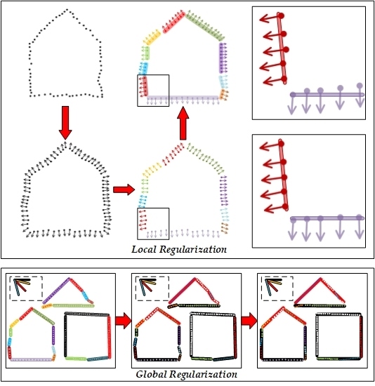
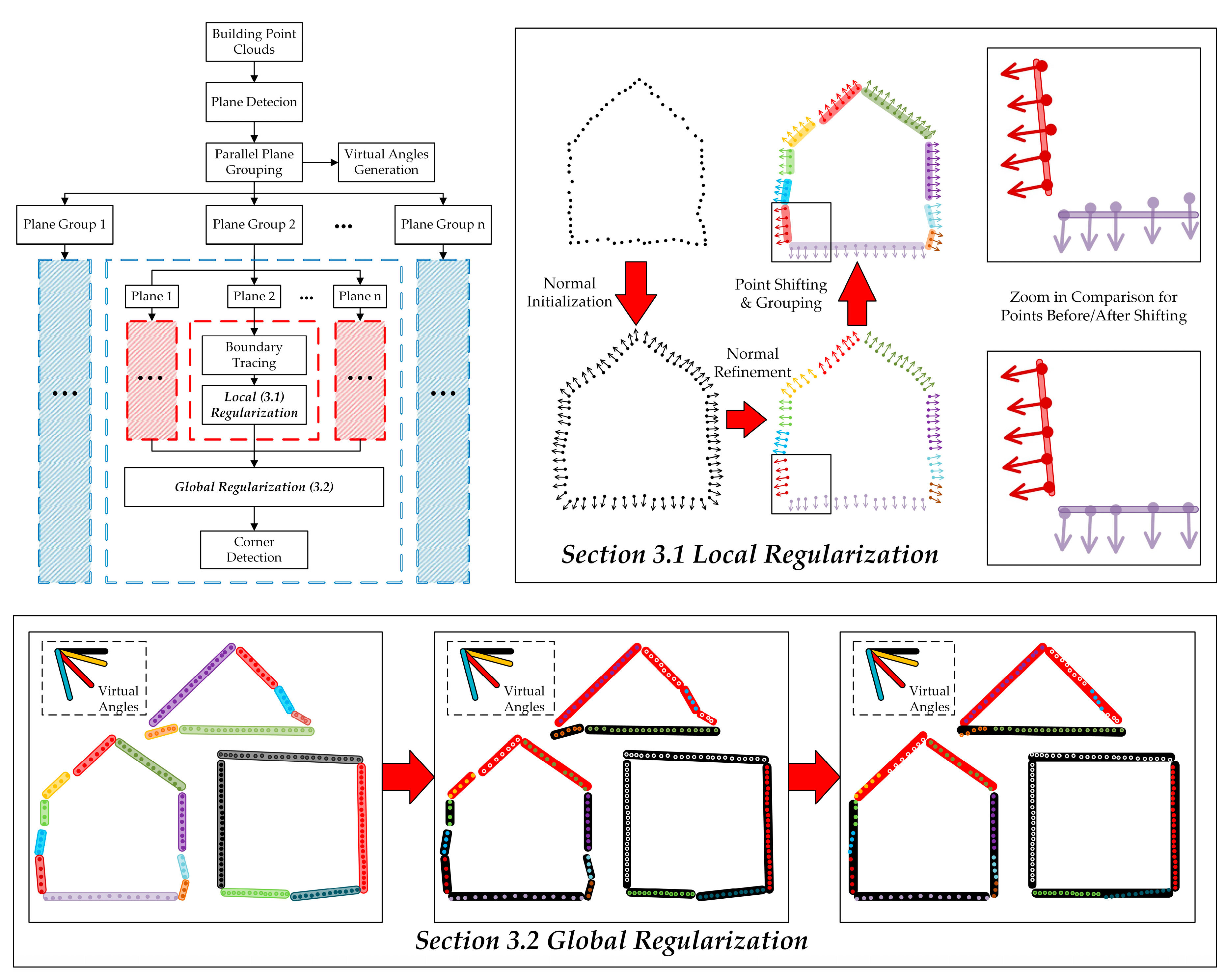
3.1. Overview of the Approach

Staring from building point clouds in one region, planar structures are first extracted with simple parallel and orthogonal constraints using the existing RANSAC-based methods [61,62]. Then, the detected 3D planes that share the same normal orientations (parallel or coplanar) are grouped to conduct boundary tracing and boundary regularization, as depicted in the blue box in Figure 2. For each plane group, 3D points are projected to 2D space by translation their centroid to the origin point and rotating the normal of the plane to the positive direction of Z-axis, the consecutive boundary points of each plane, which are the input of the proposed methods, is extracted using alpha-shapes [63]. Besides, non-parallel planes are projected to each plane group to form virtual angles for subsequent global regularization.

As shown in Figure 2, the hierarchical regularization is composed of two main stages: the local stage and the global stage. The objectives of the two stages are complementary. A closed point boundary is shifted and divided into piecewise smooth line segments in the local stage. In the global stage, global parallel and vertical relationships between line segments in the overall area are discovered to further regularize edges, which results in highly regularized polygons.

In the local stage, neighboring relationships between consecutive building boundary points are first built using a forward search strategy; then the initial normal of each point is estimated using principal component analysis (PCA) with a fixed neighbor size. Based on the initial normal orientation and the neighboring relationship, a high-quality 2D normal of each point is reconstructed by minimizing the least-squares function, which decreases the normal differences between neighboring points while ensuring that the final normal does not deviate too much from the initial value. The positions of the initial points are then shifted along the refined normal to harmonize their positions and normal orientations. These points are then grouped according to the reconstructed normal, and line segments with limited endpoints are fitted. These lines have a finite extent that is clipped to a bounding box based on the projection of the points.

In the global stage, each line segment along with its shifted points is set as an input to generate augmented line segments. The mutual parallel and vertical relations between each segment in the same group are used to form the augmentation. Besides, regularity clues from non-parallel planes are also discovered. Then, we construct an energy function that considers both data fitting cost and overall smoothness using the shifted points as observations. The energy function is minimized via graph cut and the result is highly regularized line segments in the global scene.

After the two stages of refinement, the resulting polygons are generated through a simple corner detection method that merges line segments with the same orientation and intersects. In the following section, we describe the two stages in detail.

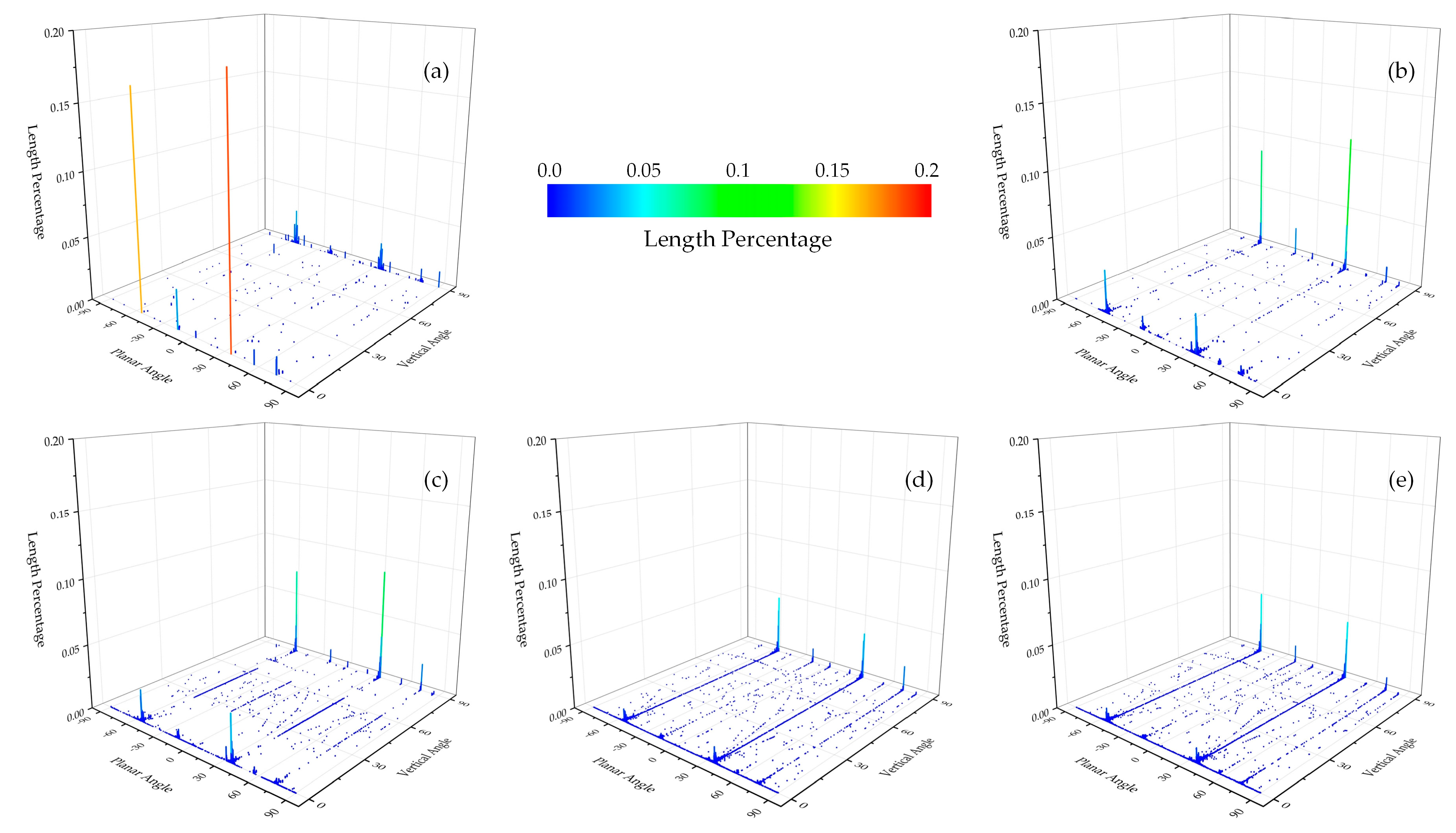
3.2. Shiftable Line Fitting for Local Regularization

The goal of this stage is to robustly reconstruct for each boundary a piecewise smooth polygon that approximates the original outline. Since the noises in point clouds may hinder the estimation of point normal, inspired by [64], the refinement of normal vectors are necessary. Therefore, three steps are incorporated to refine the boundaries and produce a piecewise smooth polygon: neighborhood estimation, normal refinement, and shiftable points grouping. A neighbor relationship between points that belong to the same line is first estimated, then the 2D normal is computed and refined based on the assumption that neighboring points are more likely to have a uniform normal (e.g., numerically the included angle is less than 1 degree). After that, piecewise smooth polylines are grouped together in accordance with their 2D normal and the positions of the points are shifted along their 2D normal based on a least-squares function that measures the consistency of points’ positions and their normal in a given tolerance which is depicted in the upper right of Figure 2. It should be noted that the shiftable line fitting is different from direct line fitting through RANSAC or other alternatives, in the ways that the proposed method are less sensitive to local noise and will create more local segments for the successive global labeling.

3.2.1. Outlier-Free Neighborhood Estimation

The main purpose of this phase is to identify outlier-free collinear relationships between consecutive points. Therefore, a forward search-based iterative method is used to estimate the neighboring region of a point which consists of collinear consecutive points around this point. The neighboring region of a given point starts from the point (itself). In each iteration, one point (the next consecutive one) is added to this region if the residual of the candidate point to the fitted least-squares linear equation of the last iteration is below a given threshold. To strictly prevent outliers and preserve sharp features, a small threshold is preferred. However, due to the discrete character of point clouds, it is meaningless to set threshold less than the Ground Sample Distance (GSD) and 1.5 GSD is chosen. The iteration stops when a candidate point is rejected, at which point the neighbor region detection of another point starts. Two points are treated as a neighborhood only when they appear in each other’s neighbor region. If a point has no neighboring points, then it is treated as a potential outlier or as high-frequency noise and is not used in subsequent processing steps. When the mutual neighbor relationships between all of the points are defined, PCA is used to estimate the initial 2D normal vector of each segment.

3.2.2. Robust Normal Estimation of Boundaries

As 2D normal can be represented by rotation angles in 1D space, we transform the normal vector into angle space, which not only decreases the number of parameters but also promotes computational efficiency. Based on the assumption that neighbor points are more likely to have similar normal, the normal angle of each point is refined in a least-squares adjustment that considers both the initial normal angle and neighbor differences. The cost function is formed based on the neighboring relationships derived in the previous step. Two terms are incorporated, as shown in Equation (1):

$$\underset{\theta }{\min }{\displaystyle \sum _{\left(p,q\right)\in N}{\omega }_{p,q}{\left|{\theta }_p-{\theta }_q\right|}^2+\lambda {\displaystyle \sum _p{\left|{\theta }_p-{\theta }_p^0\right|}^2}}$$

(1)

where N is the neighbor region and p and q are two different points which have neighbor relationships; θ_p and θ_q are the unknown normal angles of points p and q after refinement; ${\theta }_p^0$ is the initial value of θ_p; and λ controls the balance between data fidelity for initial estimated normal and consistency of normal vectors for neighbor points, a large value of λ would prevent the change of normal angle and it was set as 0.1 in all the experiments. ω is the weight between neighboring points and is computed as follows:

$${\omega }_{p,q}=e^{-{\left(\raisebox{1ex}{${\theta }_p-{\theta }_q$}\!\left/ \!\raisebox{-1ex}{$\sigma $}\right.\right)}^4}$$

(2)

where σ defines the preferred angle difference, which penalizes big initial normal differences, and fixed at 15° in all the experiments below, because we observed that the deviations of estimated normal at smooth region are lower than this value for most of the cases; θ_p and θ_q are the same as in Equation (1).

The above optimization is a standard regularized least-squares optimization and a standard solver is adopted to solve this problem [65]. The first term of Equation (1) minimizes the angle difference between neighboring points and the second term prevents the normal angles from deviating too much from their initial values. As depicted in Figure 2, after the normal refinement, the normal angle differences of the sharp features are enlarged (see the rooftop and the lower left corner), whereas those in the smooth region are reduced (see points with the same color).

3.2.3. Line Fitting with Shiftable Points

Once the high-quality normal orientations of all of the inlier points have been reconstructed, the consistent positions of boundary points p′ are updated by shifting them in the normal direction (represented by n) to smooth the initial boundary points p. The length of the shifting is quantized by a single scalar t, as p′ = p + t × n. In order to optimize the local shifting value, similar optimization is approached as defined in Equation (3). It should be noted that, unlike traditional line fitting, this procedure operates on individual point and may involve neighborhood information that does not belong to the same local segment.

$$\underset{t}{\min }{\displaystyle \sum _{\left(p,q\right)\in N}{\omega }_{pq}\left({\left|{\left({\mathit{p}}^{\prime }-{\mathit{q}}^{\prime }\right)}^T{\mathit{n}}_q\right|}^2+{\left|{\left({\mathit{q}}^{\prime }-{\mathit{p}}^{\prime }\right)}^T{\mathit{n}}_p\right|}^2\right)+\mu {\displaystyle \sum _p{t}_p^2}}$$

(3)

This is also a regularized least-squares problem, in which the weight ω is defined as the same as Equation (2) and gives larger weights to points with similar normal orientations. The left part measures the local deviation in the point’s neighboring region N, which allows smoothness across different small segments. Because there are arbitrary many solutions to this free adjustment problem, the other term is also included to ensure data fidelity by constraining the final point position so that it does not shift too much from its initial position. The scale factor μ is used to balance normal smoothness and position deviation, a large value of μ would prevent the points to shift from their initial positions.

Once the smoothed positions are obtained, piecewise smooth polylines are constructed by grouping consecutive points that share similar normal angles, as the normal angles across sharp features have been magnified in the previous step. The shifted positions of the points belonging to each group are used to fit a least-squares line segment, and the corners are detected by intersecting lines with corresponding bounding boxes, based on the projection of points. As shown in Figure 2, after the local stage simplification, the initial polygon boundary points are represented by 10 edges and the sharp features are not lost.

3.3. Constrained Model Selection for Global Regularization

In the stage described above, the consecutive boundary points are integrated as piecewise smooth line segments composed of shifted points with a finite extent and unique orientation angles. These orientation angles may be contaminated by the noise that is inherent in the initial boundary points, leading to irregular polygons.

As man-made buildings always have regular shapes and buildings in nearby regions are likely to confirm some regional level regularity, it is reasonable to infer that all of the edges from the same region of building outlines are mutual related. These kind of inter-polyline relations are mainly parallelism and orthogonality. However, non-uniform edges may also exist in building outlines, and forcing them to become parallel (or perpendicular) to the dominant orientation may induce large distortions. Therefore, in the proposed method, the regularities are only softly enforced. We cast the regularization into the label space, in which the label of two segments are considered the same if they are collinear, parallel or orthogonal. In addition, long segments are preferred in the label inferencing. This problem is, formulated as a standard MRF and solved efficiently with graph cut [66].

3.3.1 Constrained Model Extension

In our hypothesis, the line segments that constitute the same polygon only have a limited number of orientation angles, and these angles are always represented by larger edges. As the orientation of initial angles may be affected by noise, especially short edges, robust detection of inter-polyline relations is a non-trivial problem. Inspired by [57], we extend the potential orientation angle of all of the line segments according to the expected inter-polyline relations. Although only one orientation angle is selected finally, the extended orientation angles help us to recover noisy or under-sampled line segments and allow us to make global optimal orientation angle selections.

In each plane group that contains detected planes that share the same normal vector, a line segment in 2D space is represented by the corresponding point sets as p ∈ l = (c,o)^T, in which c is the center position of the segment and o is the orientation angle of this line segment. In order to enhance the regularities, only a subset of all the possible values for the orientations should be selected. Therefore, all the orientations are first extended to pairs, which also consider the corresponding orthogonal direction as ϕ = [o, o ± π/2]. The sign of the extended value is chosen properly so that the two orientations all fit into the range of [0,π). Then the label space, Φ, is the union set of two parts Φ₁ and Φ₂. One part is formulated by all the pairs for all the segments as Φ₁ = {ϕ₁ⁱ|i = 1, 2…, M} and M is the total number of segments in this plane group. The other part, nominated as virtual angles in this paper, is formulated by the projections from non-parallel plane groups in the same region as Φ₂ = {ϕ₁ⁱ|i = 1, 2…, N} and N is the total number of plane groups that are not parallel with this plane group. Since building outlines are always mutual appeared in intersected planes and the function of a plane is estimated by a distinct larger amount of points than the function of a line segment, the label space in Φ₂ is more likely to reveal the real orientations.

In the model extension process, the center positions remain unchanged and only the orientation angles for each segment varies according to the selected label. Note that for a given original model and a given candidate angle, only one candidate model can be formed, either parallel or perpendicular. The purpose of the model extension is to ensure that the optimal configuration exists as a subset of the augmented candidate model set and that a regularized polygon can be simultaneously recovered by applying a proper model selection strategy.

3.3.2 Model Selection Using Graph Cut

Next, we need to select the optimal models from the extended candidate models. An initial model can only correspond to one final selected model. An energy function that considers both neighbor smoothness and data fitting degree is built to measure the regularity and data fitting errors, as below:

$$\begin{array}{l}E\left(\phi \right)={\displaystyle \sum _{l\in L}D\left(l,{\phi }_l\right)}+\lambda {\displaystyle \sum _{\left(l,k\right)\in S}{e}^{\left(-\raisebox{1ex}{$\left|{\phi }_l-{\phi }_k\right|$}\!\left/ \!\raisebox{-1ex}{$\sigma $}\right.\right)}}\\ D\left(l,{\phi }_l\right)={\displaystyle \sum _{p\in l}{d}_{\perp }^{{\phi }_l}\left(p\right)}\end{array}$$

(4)

in which, L represents all the line segments in this plane group and l is a line segment which is fitted by several shifted points. The first term measures the refitted error of the line segments, using the selected label orientation and means the distance of a point to the corresponding segments. And the second is the smoothness constraint, which penalizes similar initial angle models that are labeled differently. S defines the pairwise neighborhood of the segments, which includes pairs of models that have similar initial orientation angles; σ is the same as in Equation (2) (15° selected for all the experiments in this paper). λ controls the strength of the regularities, and if the value of λ is set to 0, non-regularity are considered in the optimization process.

We implement the graph cut algorithm [66,67] to minimize the energy function and convert the labeling result to corresponding orientation angles. Successive segments with the same orientations are merged to form a new segment and the corners are identified as the intersection of two non-parallel line segments. As depicted in Figure 2, after the global stage regularization, the piecewise smooth polygons are further merged and intersected to form new polygons with two orientation angles that represent the main structure of the original point boundary while preserving the parallel and perpendicular relationships between the main edges.

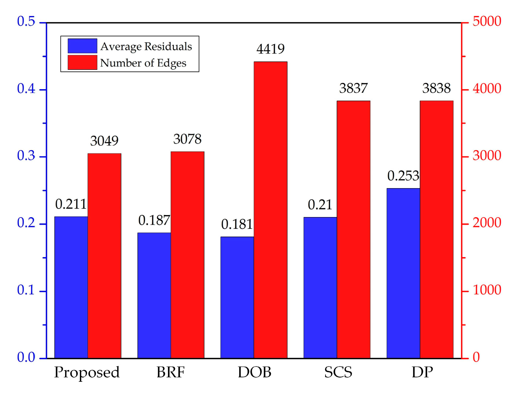
4. Experimental Evaluation

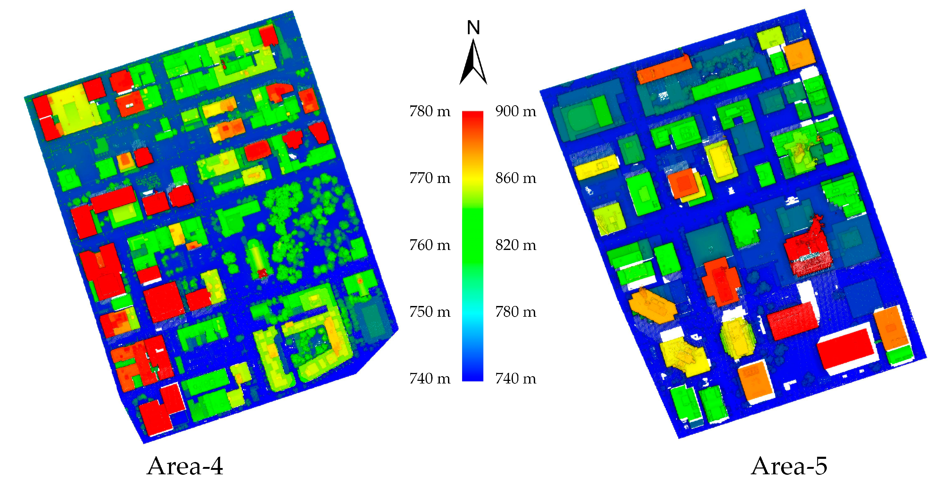
4.1. Description of the Test Data and Evaluation Methods

To test our algorithm, we evaluate the performance in two different application contexts: 2D building footprint generalization and 3D building model reconstruction. Furthermore, we use both photogrammetric point clouds generated from aerial oblique images and ALS data to test the robustness to the different type of noises. The datasets all cover urban areas, such as Hong Kong, and Toronto [68].

The generation of photogrammetric point clouds for the Hong Kong datasets is accomplished using off-the-shelves SfM/MVS solutions [69]. And, in the pre-processing, the building point clouds are extracted using existing footprints and post-processing interactions. After that, planes are detected via RANSAC [61,62,70]. In addition, other powerful methods could replace the methods we have chosen in this study. Planes which share the same normal are grouped together to be further regularized and the virtual angle between intersected plane groups are computed. For each plane group, the detected planes are first rotated and transformed into 2D space; then, border points are extracted by applying the 2D alpha-shapes. After regularization, the 2D polygons are transformed back into 3D space. The buildings and corresponding plane segmentations are illustrated in Figure 3, and their basic information is given in

Table 1. Basic information about the photogrammetric test datasets.

Area Name	Point Number	Point Density (pt/m2)	Detected Planes (Groups)
Centre	3,005,398	81	381 (29)

.

This study also tests the performance of the ALS dataset in 2D footprint generalization. The ALS data for two areas are acquired from downtown Toronto. The dataset was released by ISPRS [68] and two areas called Area-4 and Area-5 are used. Building points are extracted using existing building detection methods [71], then manually refined to correct some apparent mistakes (e.g., remove false detection and restore incomplete detection). Then, single buildings are obtained through point clustering and all of the points are projected to the ground plane to conduct boundary extraction and regularization. The ALS point clouds being tested are shown in Figure 4 and their basic information is given in

Table 2. Basic information about the ALS test datasets.

Area Name	Point Number	Point Density (pt/m2)	Detected Planes (Groups)
Area-4	1,291,120	6.15	45 (1)
Area-5	1,138,977	5.42	34 (1)

.

We compare our algorithm with four representative methods. The first compared method is the well-known Douglas–Peucker (DP) algorithm (with the threshold from 0.2 m to 0.35 m in most cases) [27] and the second compared method is a polygon simplification algorithm published by [31] which we represent as SCS in the following part of this paper. The virtue of these two methods is to maintain of good approximation error and produce simplified polygons with approving data fidelity to the input boundary. Besides, we also compared with regularity-skilled methods, e.g., the dominant orientation based methods [47] (represent as DOB), and a method which balanced between regularity and fidelity [20] (represent as BRF). To give a fair comparison between different polyline simplification and regularization algorithms, the polygons are simplified to similar numbers of vertexes, e.g., changing the parameters in an adaptive manner. Both qualitative and quantitative comparisons are conducted. The output polygons are displayed in their original 3D or 2D space and are compared visually. In order to reveal to what extent do the output polygons approximate the input boundary (fidelity) and how regular do the polygons are (regularity), two indices are calculated to quantitatively measure them respectively. Fidelity is defined by the averages of the distances from the original boundary points to their corresponding output polylines, and regularity is represented by the distribution of the orientation angles that appear in each output polygon. Since the ALS datasets in Toronto are released with ground truth [68], the results are further investigated by calculating the root mean square (RMS) distance and the Hausdorff distance [72] to the reference boundaries. Note that, only footprints with 1:1 correspondence to the reference datasets are incorporated in the comparison.

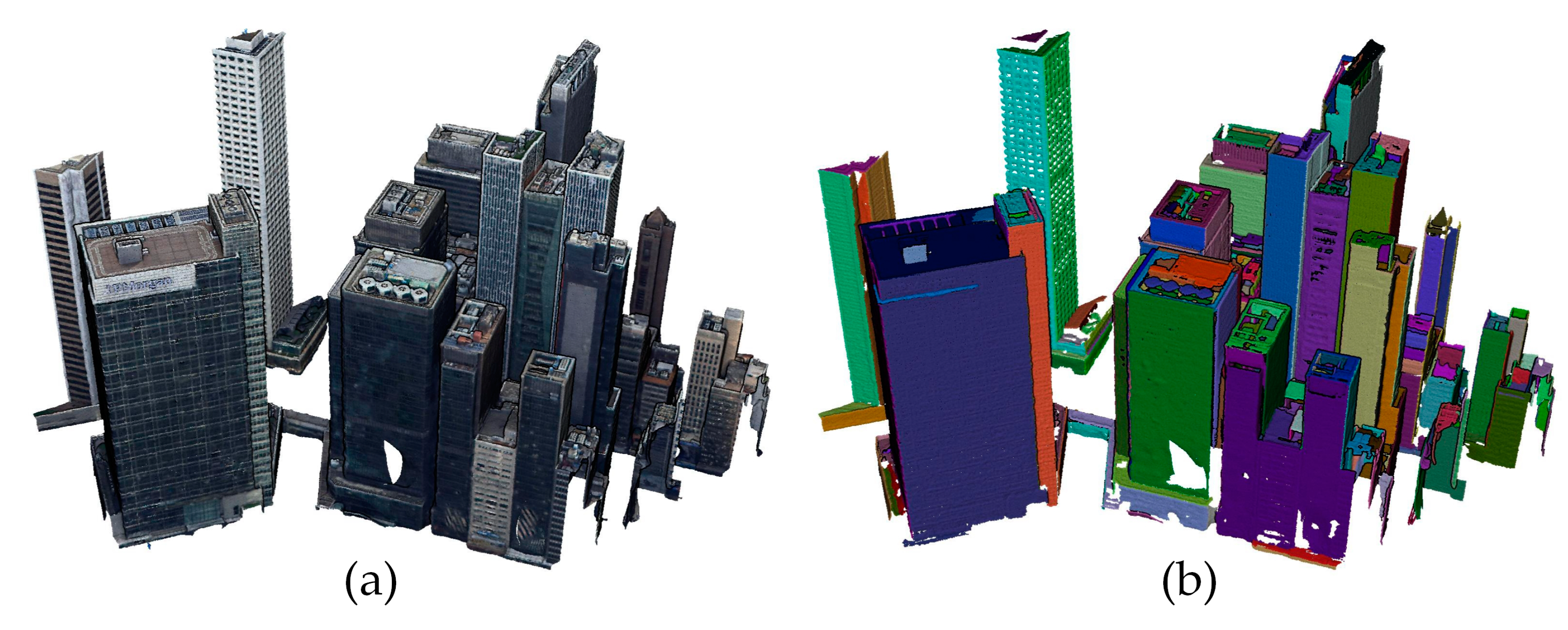
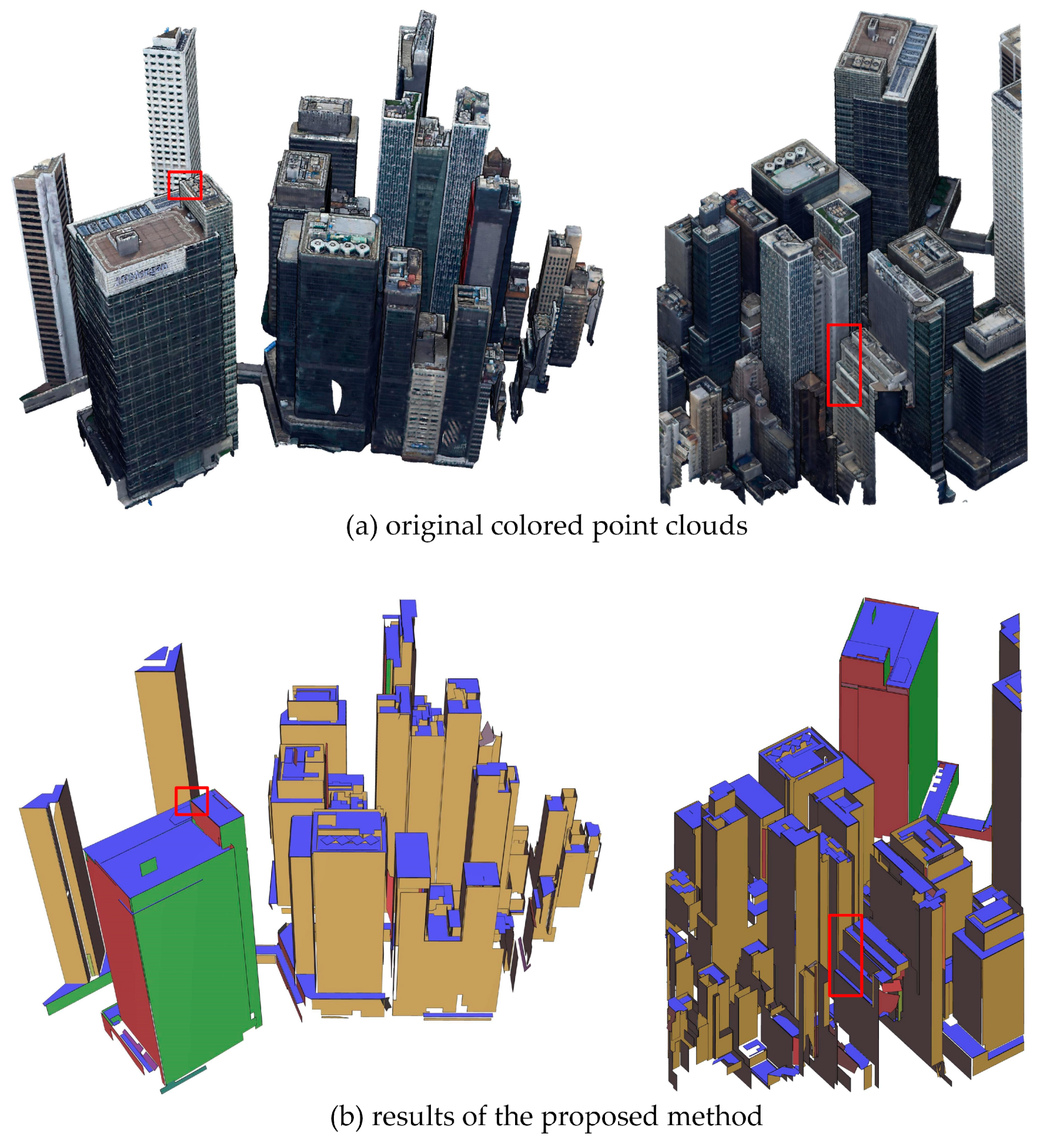
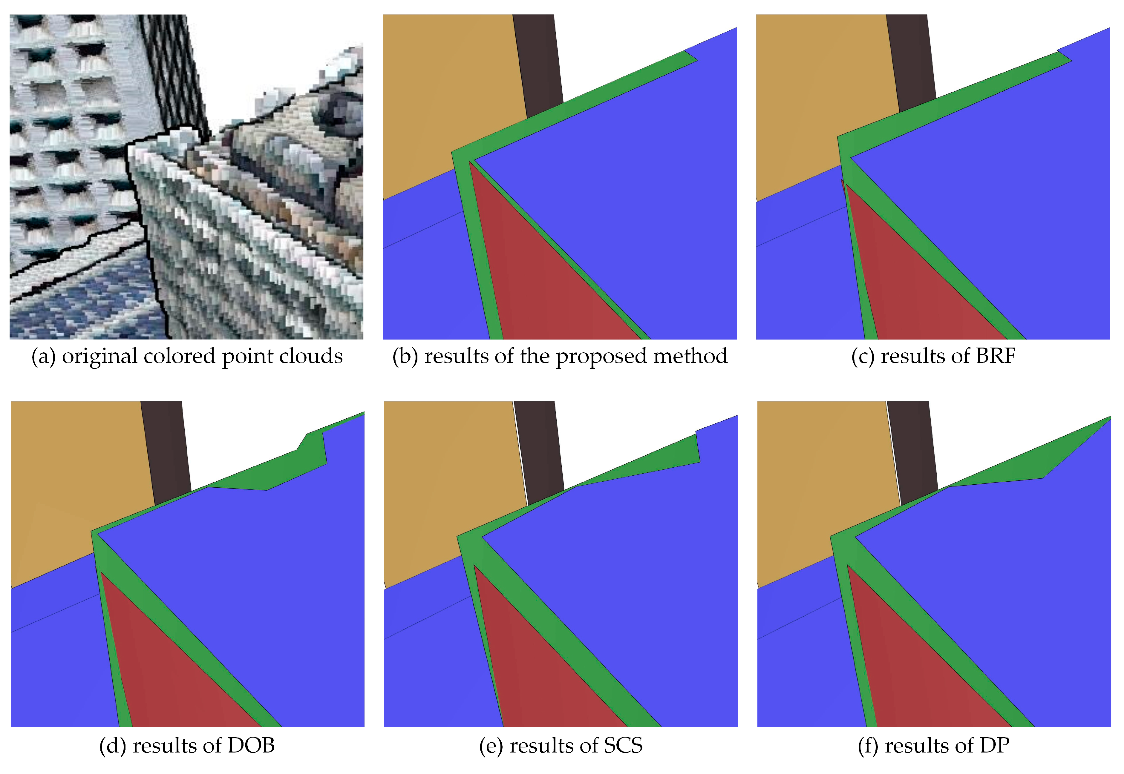
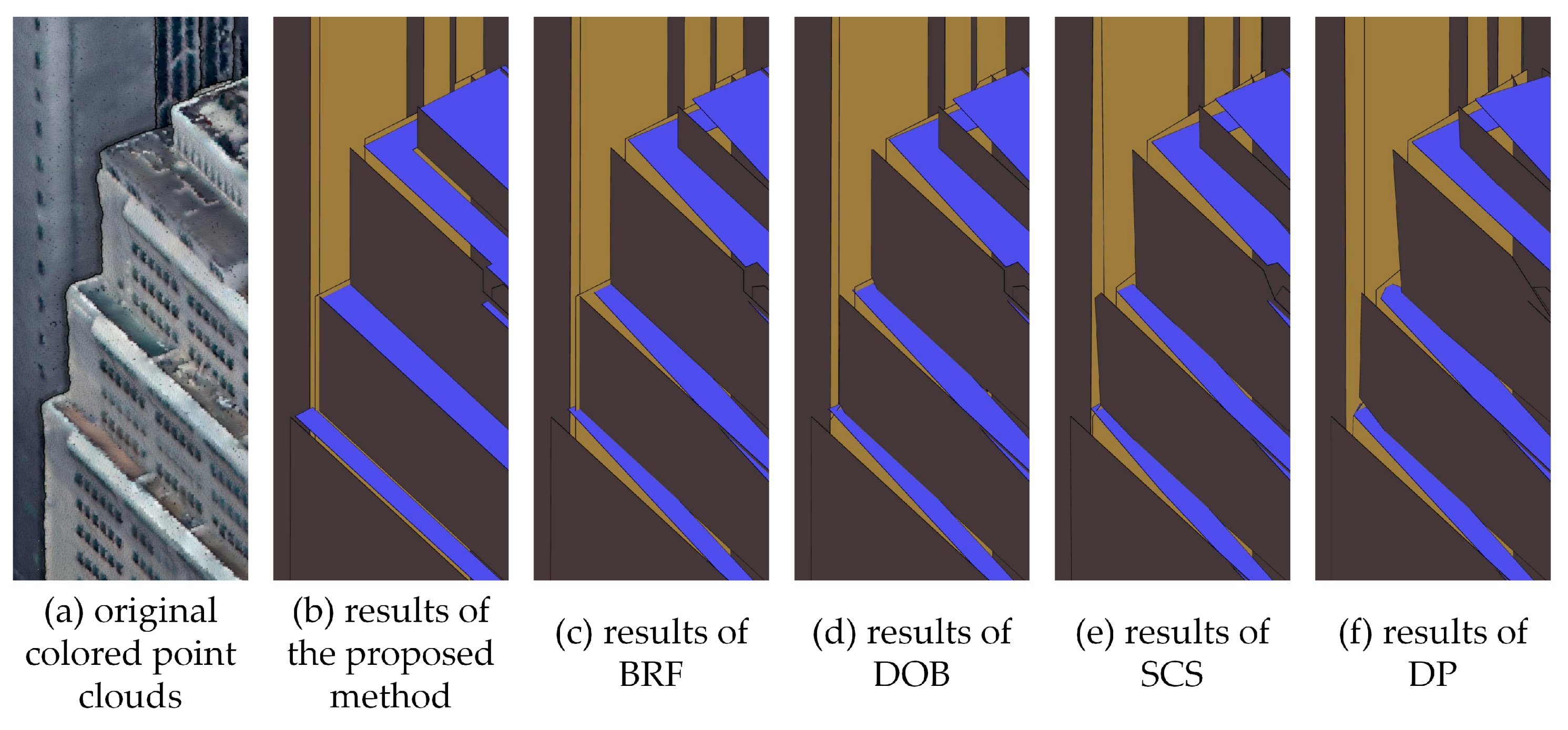
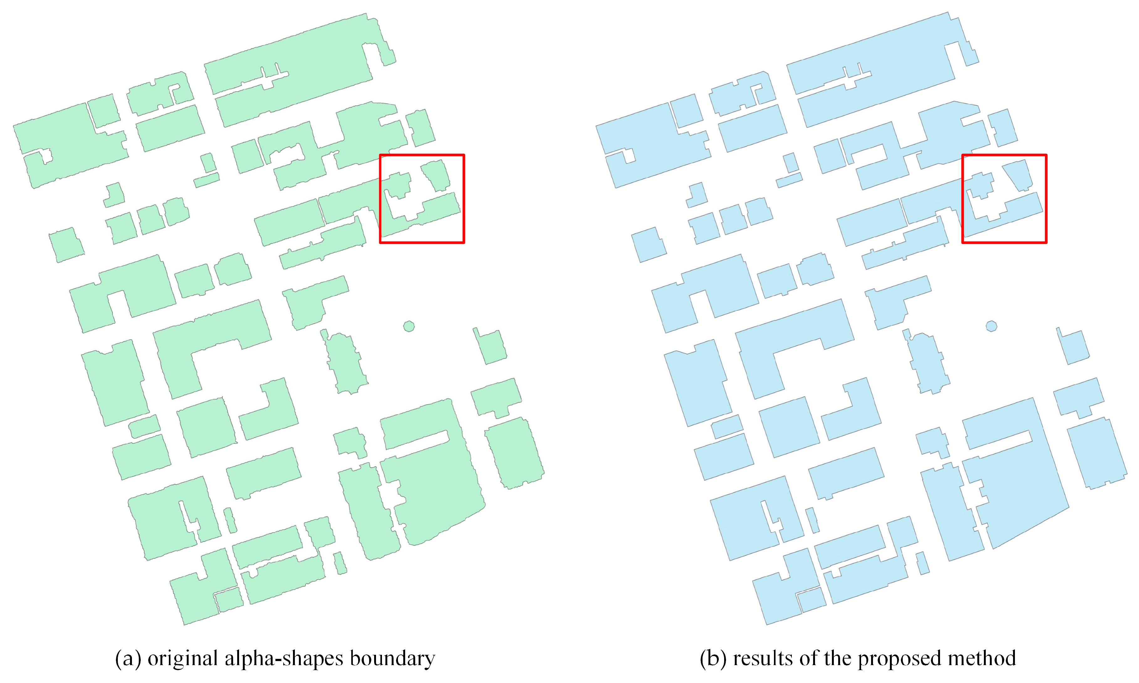
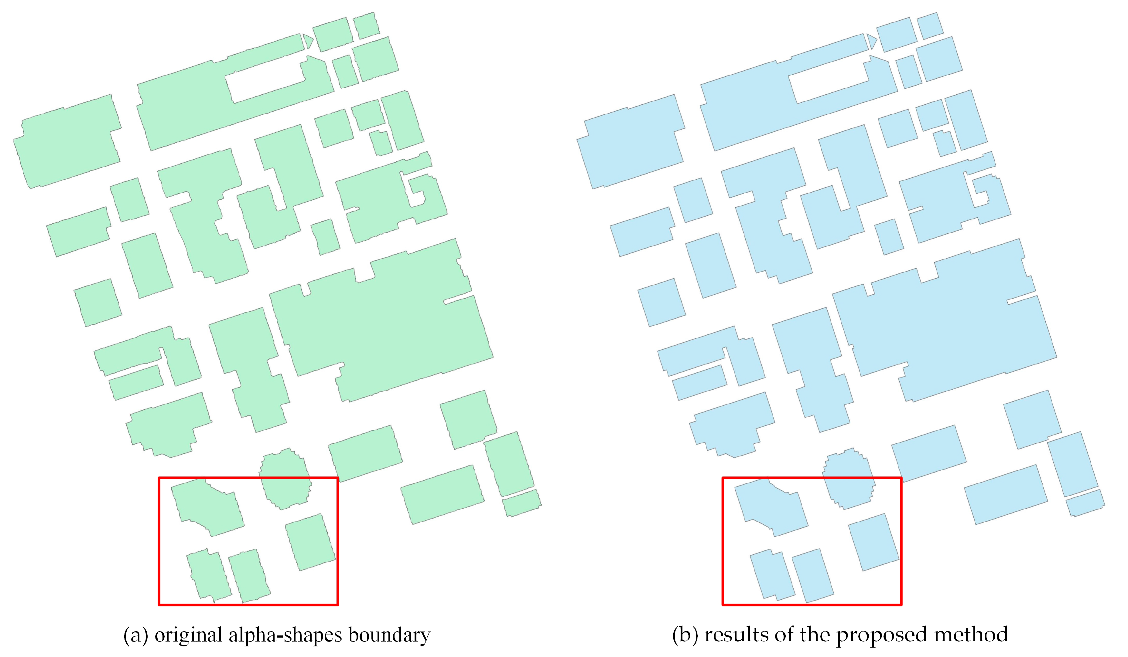
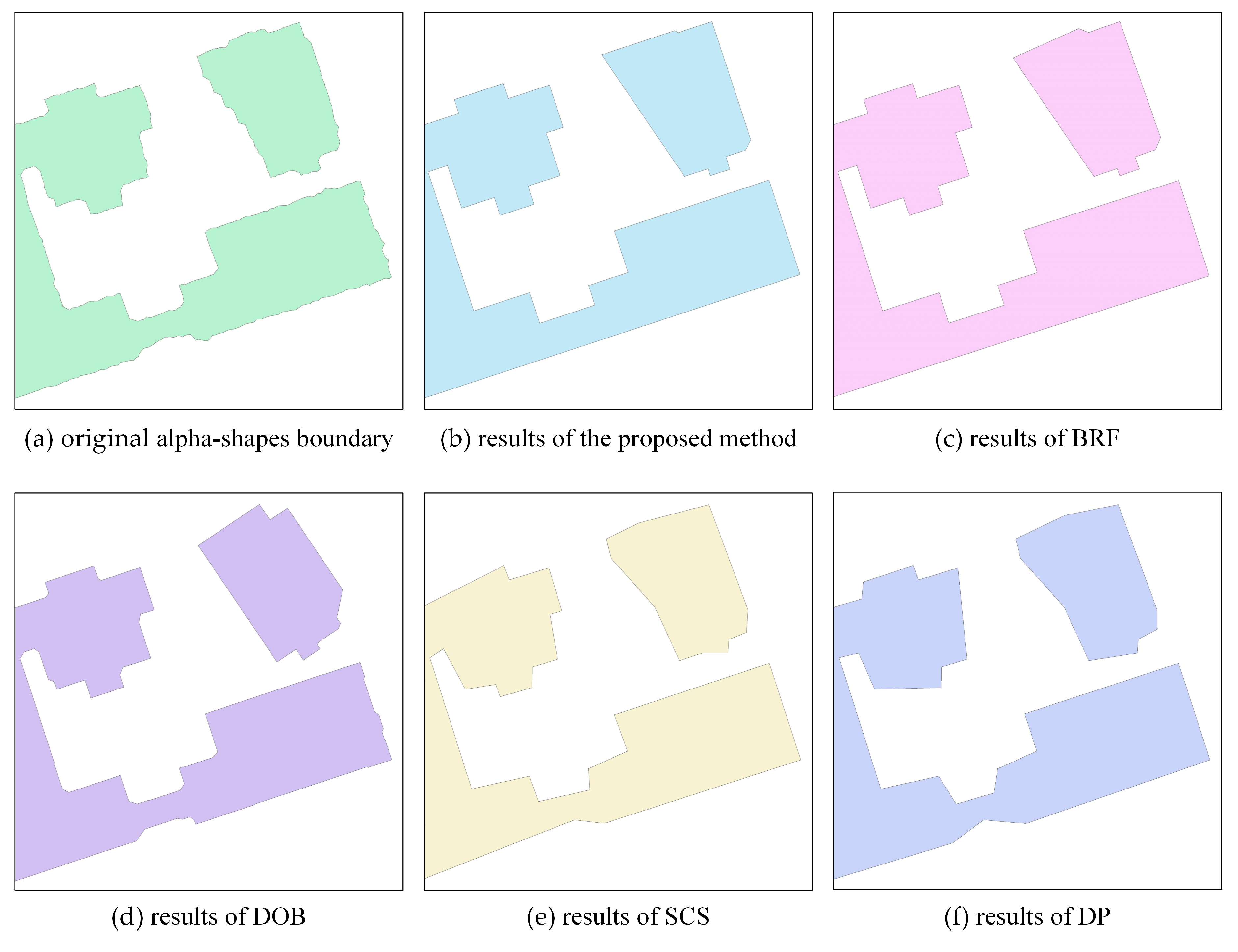
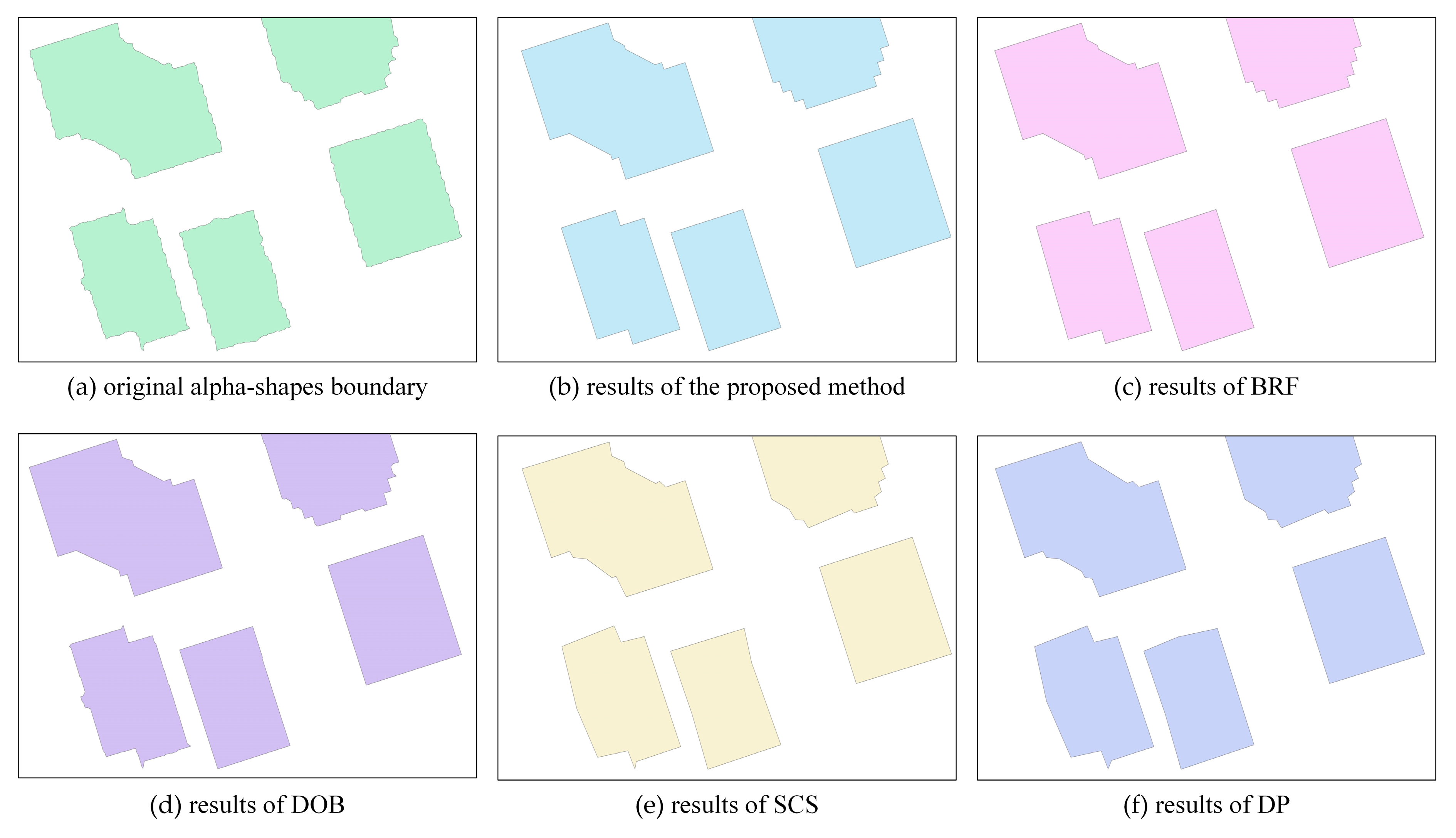
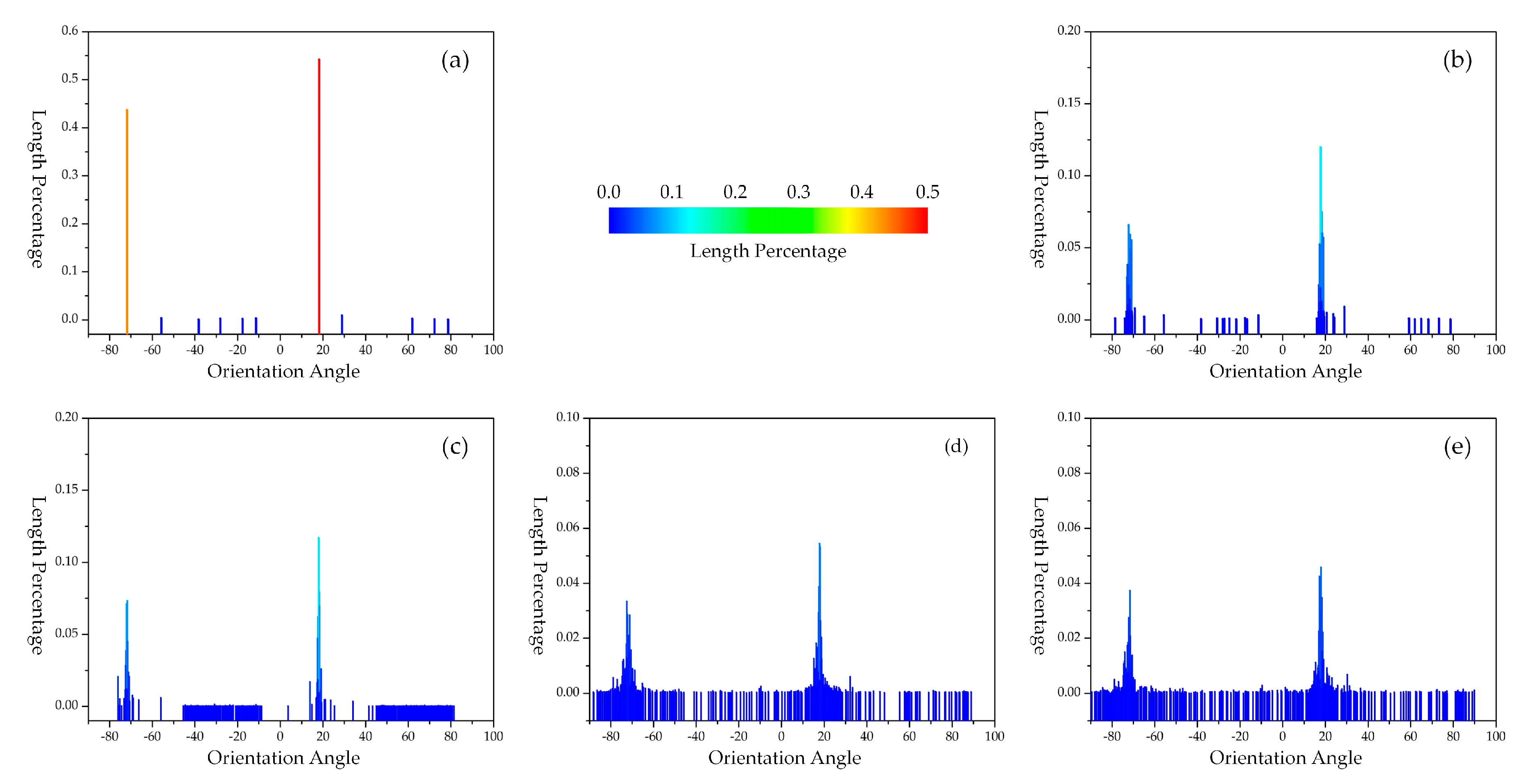
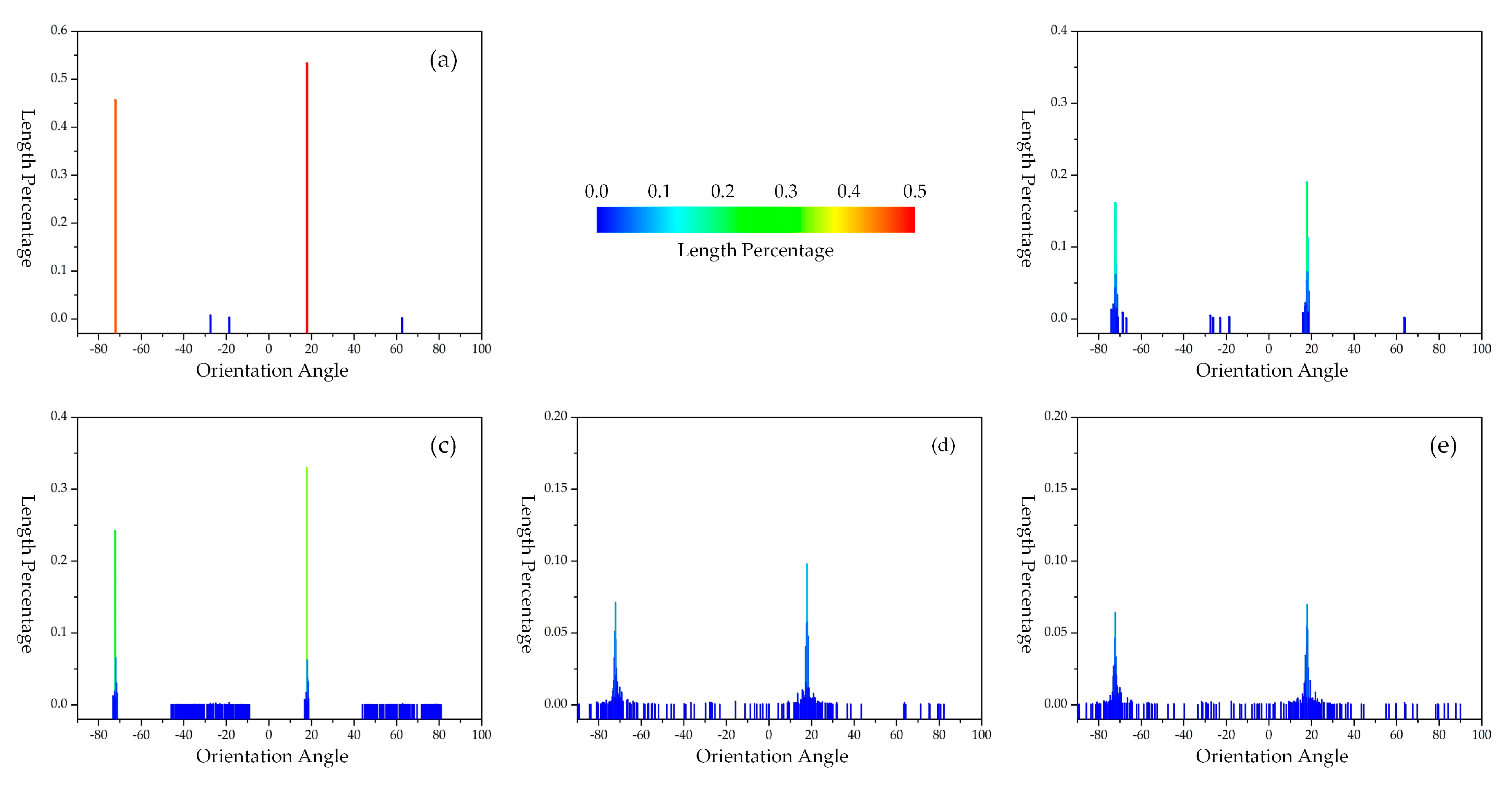
4.2. Experimental Comparison of the Photogrammetric Point Clouds

As shown in Figure 5, the proposed method could produce neat polygons with a good quality that main structures of buildings are rather recognizable. The detailed comparisons for all the five tested methods are shown in Figure 6 and Figure 7. Although all the five tested algorithms can simplify the polygon outlines to a certain degree, their visual qualities are different in detail. Since regularity constraints are not enforced, the results from SCS and DP could only recover the shape with approving errors, the parallel and the orthogonal relationship between edges are not preserved.

Meanwhile, for most rectangules the proposed methods and the method in BRF and DOB could correctly recover edges which belong to the major orientations. However, as non-dominant orientations are kept with their original orientations to receive a higher degree of data fidelity in DOB, the output polygons may contain a lot of tilt edges without mutual regularity. In contrast, the proposed methods and BRF could discover regularity constraints between non-dominant orientation edges and softly enforce mutual regularity constraints, resulting in polygons with overall inner regularity. When comparing reconstructed polygons in 3D, it is obvious that corners which shared by three planes are visually recognized from the proposed methods, the mutual orthogonal relationship between edges belong to different planes are also recovered as the intersection angles between different plane groups are served as virtual orientation angles in the global optimization process. This feature is potentially useful for topology reconstruction between polygons. Some polygon-snapping algorithms could use the results of our algorithm as input [56]. As shown in Figure 6 and Figure 7, results from BRF, DOB, SCS, and DP are somehow irregular at building corners due to the inaccurate estimation of dominant orientation in noisy point clouds.

The quantified fidelity evaluation is presented in Figure 8. As shown in the graph, for all five tested methods, the average residuals of the output polygon ranges from 0.181 m to 0.253 m while the numbers of edges are between 3049 and 4019. The number of edges for the proposed method is the smallest among all the five methods, stating that the output polygons of our method are quite concise. As for residuals, the minimum average value is 0.181 m which obtained by DOB and the value for the proposed method is slightly larger than that value (3 cm), which indicates a satisfying data fidelity of the output polygons by the proposed method.

In Figure 9, we illustrate the distribution of the orientation angles that appear in the output polygons. Orientation angles with intersection angle less than 0.1 degrees are identified as the same orientation angle. And, for same orientation angles, the length of their line segments are accumulated and divided by the total length of polygons in the scene to get the length percentage for this orientation angle. As shown in Figure 9, the proposed methods produce polygons with the minimum number of orientation angles and 1/3 of the total edges (in length) are shared by two orientation angles which orthogonal with each other. For the other four tested methods, orientation angles also concentred on several orientations but with less affinity. For DOB, edges belong to the dominant orientation are detected and complied, however, the remained edges are still irregular. Meanwhile, for BRF, several distinctive orientations for individual polygons are recovered but lacks inter-polygon regularity. As illustrated in Figure 9d,e, results from SCS and DP which focus on data approximation, regularity is not considered. The statistical values in Figure 8 and Figure 9 indicate that our method produces global regularized polygons that fit the original point boundaries well and maintain data fidelity to a competitive degree, which conforms to the visual observations in Figure 5, Figure 6 and Figure 7.

4.3. Experimental Comparison of ALS Point Clouds

The original alpha-shapes boundary of the 2D footprints from Area-4 and Area-5, together with the corresponding generalized polygons produced by the proposed method are shown in Figure 10 and Figure 11, respectively. Detailed areas of the two environments are presented in Figure 12 and Figure 13, respectively. Overall, all of the five methods are capable of generalizing building footprints while maintaining the main structure. Long edges are simplified with good data fidelity due to the preferable sampling of the original ALS data. However, the results of the detailed reconstructions of the short edges are different. Shorter edges, which are not as densely sampled as longer ones, are neatly reconstructed in the polygons produced by the proposed method, BRF, and DOB, but are distorted or deformed in the polygons produced by SCS and DP. For rectangular footprints, the output polygons for the Manhattan-based method are concise and regular. However, some tilt edges are not regularized, see Figure 12 and Figure 13. As for the proposed method, nearly all the major structure of original boundaries are well preserved. Potential regularity between edges are discovered to enhance regularity, and non-dominant orientations are preserved to a large degree.

The quantified fidelity evaluations of Area-4 and Area-5 are presented in Figure 14. As shown in the bar graph, for the polygons in Area-4 and Area-5, the RMS of the output polygons (setting the original boundary points as references) produced by the five methods are all lower than 0.3 m, and the overall residuals for Area-5 are lower than Area-4. Given the point density in the original ALS data (see Table 2), these results are relatively good. In both the two areas the output edge numbers of the proposed method are the smallest while the residuals for the proposed methods remain a comparable low level among the five test method, proving again the preferable fidelity of boundaries after the two-stage regularization. In the meantime, results for the Manhattan-based method in DOB is low indeed for they keep too many edges with original orientation angles. As a result, the output polygons by DOB contain the largest number of edges. Since the point density is relatively low, SCS and DP may lose sharp features and result in distorted polygons with large data fitting residuals.

In addition, we calculate the RMS and Hausdorff distance of the output polygons by comparing with the ground truth provided by the benchmark sponsors [68]. Apart from evaluating the performance of the five test methods, the RMS values are also compared with other benchmark participants’ results reported in their publications [73,74,75]. As shown in

Table 3. Comparison of the root mean square (RMS) and Hausdorff distance in Area-4.

Method	RMS (m)	Hausdorff Distance (m)
Proposed	0.77	1.28
BRF [20]	0.79	1.35
DOB [47]	1.11	2.01
SCS [31]	0.94	1.56
DP [27]	1.09	1.86
CKU [73]	1.62	--
YOR [74]	0.80	--
MON2 [75]	0.96	--

and

Table 4. Comparison of the RMS and Hausdorff distance in Area-5.

Method	RMS (m)	Hausdorff Distance (m)
Proposed	0.68	1.13
BRF [20]	0.68	1.14
DOB [47]	1.02	2.00
SCS [31]	0.91	1.31
DP [27]	0.93	1.43
CKU [73]	1.68	--
YOR [74]	0.90	--
MON2 [75]	0.89	--

, the RMS for the proposed method is about 0.77 m in Area-4 and 0.68 m in Area-5 while the Hausdorff distances to the ground truth polygons are 1.28 m and 1.13 m, respectively. In all the five tested methods, the RMS and Hausdorff distance of the proposed method is the lowest in both the two test ALS areas, demonstrate that our method can outperform other boundary simplification and regularization methods. When comparing with other results which focus on building detection, the RMS value of the proposed method still shows comparative results. The reason may lie in the fact that the input building point clouds in this paper are extracted with manual post-processing, thus the input boundaries used here are more intact.

In Figure 15 and Figure 16, we present the distribution graph of the orientation angles that appear in the output polygons. In Area-4, the output polygons produced by the proposed method are concentrated on 11 orientation angles and two of which, that deviate from each other by 90 degrees, contain more than 90% of edges in length. Meanwhile, in Area-5, our method produced polygons are concentrated on only five orientation angles. The resulting orientation angle histogram of BRF and DOB also show peaks at the two dominant orientations of the scene, but as inter-polygon constraints are not enforced, the regional level regularity is not preserved as well as the proposed method. As for the methods in SCS and DP, due to the low point density, the loss of sharp feature around corners result in irregular boundaries for small edges which are not well-sampled.

5. Discussions

The experiments on photogrammetric and ALS point clouds revealed that the output polygons for the proposed methods have presented better regularities than other methods. Although, in Figure 8 and Figure 14, the average residuals for the proposed methods are larger than those for BRF [20] and DOB [47], it should be noted that, in these two experiments, the original boundary points are set as references to reveal absolute data fidelity; and the data fidelity and regularities are two competed desires. However, if using the ground truth labeled manually as the reference, the RMS values for the proposed methods became the smallest. This suggests that the proposed methods could resist the noise in original boundary and produce regularized polygons with inter-part regularity, see Figure 9, Figure 15, and Figure 16. Meanwhile, the Hausdorff distance which measures shape similarity also confirmed that the results of the proposed methods are the most similar with ground truth in shapes.

Besides, the parameters of the proposed method could be changed regarding the property of input point clouds and surveying area. In our test, the parameters setting strategy used in this paper are quite robust for the three test areas. The reason might be that these parameters stand for some physical meaning which descript the surveyed objects or the input point clouds.

However, there are also some limitations of the proposed methods. Firstly, compared with BRF [20], DOB [47], SCS [31], and DP [27], which regularized each plane of a single building separately, the proposed method works on the whole datasets (in the global stage) and computational complexity increased quadratically with the number of segments. Thus, further incremental processing strategy should be considered to make the method scalable to large datasets. Secondly, the extraction of planes from the point clouds, as a pre-processing stage for the proposed methods, is still an open problem in city scale, especially for the buildings with many fragmented parts.

6. Conclusions

In this study, a method for the hierarchical regularization of noise boundaries of buildings from ALS and photogrammetric large scale point clouds is presented. The method incorporates two stages of regularization that reconstruct piecewise smooth line segments and global regularized polygons in regional level. Qualitative and quantitative comparisons of the proposed method with existing methods have revealed the effectiveness of the proposed method in handling highly noisy point boundaries and producing polygons with both satisfactory regularity and data fidelity. The regularized polygons could fit original boundary points with 0.2 m in average residual while making more than 90% of edges to be regular (either parallel or orthogonal) with each other. The absolute RMS refers to ground truth is about 0.7m and the shape similarity is about 1.2 m in the Hausdorff distance.

In the future, three related problems should be solved. First, rather than just planar primitives, more complex regularities, such as concentric of sphere, cone, and cylinder, may also be investigated. Second, rather than the volumetric segmentation or 3D plane arrangement [55] approaches for building reconstruction, which is hard for interactively intervention when the quality of extracted plane is less desirable, the reconstructed polygons will be explored in an interactive environment, which is more practical in real-world applications. Third, alternative reconstruction paradigms, e.g., 3D edge extraction from point clouds then reconstruct building faces from closed edges, may also be incorporated with the hierarchical regularization methods to produce precision 3D models.

References

- Vosselman, G.; Maas, H. Airborne and Terrestrial Laser Scanning; Whittles Publishing: Caithness, UK, 2010; p. 336. [Google Scholar]
- Berger, M.; Tagliasacchi, A.; Seversky, L.; Alliez, P.; Levine, J.; Sharf, A.; Silva, C. State of the art in surface reconstruction from point clouds. In EUROGRAPHICS Star Reports; The Eurographics Association: Geneve, Switzerland, 2014; pp. 161–185. [Google Scholar]
- Moulon, P.; Monasse, P.; Marlet, R. Global fusion of relative motions for robust, accurate and scalable structure from motion. In Proceedings of the IEEE International Conference on Computer Vision (ICCV), Sydney, Australia, 1–8 December 2013; pp. 3248–3255. [Google Scholar]
- Vu, H.; Labatut, P.; Pons, J.; Keriven, R. High accuracy and visibility-consistent dense multiview stereo. IEEE Trans. Pattern Anal. Mach. Intell. 2012, 34, 889–901. [Google Scholar] [CrossRef] [PubMed]
- Hu, H.; Zhu, Q.; Du, Z.; Zhang, Y.; Ding, Y. Reliable spatial relationship constrained feature point matching of oblique aerial images. Photogramm. Eng. Remote Sens. 2015, 81, 49–58. [Google Scholar] [CrossRef]
- Rupnik, E.; Nex, F.; Toschi, I.; Remondino, F. Aerial multi-camera systems: Accuracy and block triangulation issues. ISPRS J. Photogramm. Remote Sens. 2015, 101, 233–246. [Google Scholar] [CrossRef]
- Xie, L.; Hu, H.; Wang, J.; Zhu, Q.; Chen, M. An asymmetric re-weighting method for the precision combined bundle adjustment of aerial oblique images. ISPRS J. Photogramm. Remote Sens. 2016, 117, 92–107. [Google Scholar] [CrossRef]
- Hirschmuller, H. Stereo processing by semiglobal matching and mutual information. IEEE Trans. Pattern Anal. Mach. Intell. 2008, 30, 328–341. [Google Scholar] [CrossRef] [PubMed]
- Hu, H.; Chen, C.; Wu, B.; Yang, X.; Zhu, Q.; Ding, Y. Texture-aware dense image matching using ternary census transform. ISPRS Ann. Photogramm. Remote Sens. Spat. Inf. Sci. 2016, 3, 59–66. [Google Scholar] [CrossRef]
- Zlatanova, S.; Rahman, A.A.; Shi, W. Topological models and frameworks for 3D spatial objects. Comput. Geosci. 2004, 30, 419–428. [Google Scholar] [CrossRef] [Green Version]
- Biljecki, F.; Ledoux, H.; Stoter, J. An improved LOD specification for 3D building models. Comput. Environ. Urban Syst. 2016, 59, 25–37. [Google Scholar] [CrossRef] [Green Version]
- Singh, S.P.; Jain, K.; Mandla, V.R. Virtual 3D city modeling: Techniques and applications. ISPRS-Int. Arch. Photogramm. Remote Sens. Spat. Inf. Sci. 2013, 2, 73–91. [Google Scholar] [CrossRef]
- Biljecki, F.; Stoter, J.; Ledoux, H.; Zlatanova, S.; Çöltekin, A. Applications of 3D City Models: State of the Art Review. ISPRS Int. J. Geo-Inf. 2015, 4, 2842–2889. [Google Scholar] [CrossRef] [Green Version]
- Poux, F.; Neuville, R.; Nys, G.; Billen, R. 3D Point Cloud Semantic Modelling: Integrated Framework for Indoor Spaces and Furniture. Remote Sens. 2018, 10, 1412. [Google Scholar] [CrossRef]
- Bosche, F.; Haas, C.T.; Akinci, B. Automated recognition of 3D CAD objects in site laser scans for project 3D status visualization and performance control. J. Comput. Civ. Eng. 2009, 23, 311–318. [Google Scholar] [CrossRef]
- Lafarge, F.; Mallet, C. Creating large-scale city models from 3D-point clouds: A Robust Approach with Hybrid Representation. Int. J. Comput. Vis. 2012, 99, 69–85. [Google Scholar] [CrossRef]
- Albers, B.; Kada, M.; Wichmann, A. Automatic extraction and regularization of building outlines from airborne LIDAR point clouds. In Proceedings of the 2016 XXIII ISPRS Congress, Prague, Czech Republic, 12–19 July 2016. [Google Scholar]
- Cabral, R.; Furukawa, Y. Piecewise planar and compact floorplan reconstruction from images. In Proceedings of the IEEE Conference on Computer Vision and Pattern Recognition (CVPR), Columbus, OH, USA, 23–28 June 2014; pp. 628–635. [Google Scholar]
- Lee, J.; Han, S.; Byun, Y.; Kim, Y. Extraction and regularization of various building boundaries with complex shapes utilizing distribution characteristics of airborne LIDAR points. ETRI J. 2011, 33, 547–557. [Google Scholar] [CrossRef]
- Xie, L.; Hu, H.; Zhu, Q.; Wu, B.; Zhang, Y. Hierarchical regularization of polygons for photogrammetric point clouds of oblique images. ISPRS-Int. Arch. Photogramm. Remote Sens. Spat. Inf. Sci. 2017, 42, 35–40. [Google Scholar] [CrossRef]
- Li, Z.; Openshaw, S. Algorithms for automated line generalization1 based on a natural principle of objective generalization. Int. J. Geogr. Inf. Syst. 1992, 6, 373–389. [Google Scholar] [CrossRef]
- Garrido, A.; Garcia-Silvente, M. Boundary simplification using a multiscale dominant-point detection algorithm. Pattern Recog. 1998, 31, 791–804. [Google Scholar] [CrossRef]
- Sester, M. Optimization approaches for generalization and data abstraction. Int. J. Geogr. Inf. Sci. 2005, 19, 871–897. [Google Scholar] [CrossRef]
- Xie, J.; Feng, C. An integrated simplification approach for 3D buildings with sloped and flat roofs. ISPRS Int. J. Geo-Inf. 2016, 5, 128. [Google Scholar] [CrossRef]
- Kada, M.; Luo, F. Generalisation of building ground plans using half-spaces. Int. Arch. Photogram. Remote Sens. Spat. Inf. Sci. 2006, 36, 2–5. [Google Scholar]
- Xiao, Y.; Wang, C.; Li, J.; Zhang, W.; Xi, X.; Wang, C.; Dong, P. Building segmentation and modeling from airborne LiDAR data. Int. J. Digit. Earth 2015, 8, 694–709. [Google Scholar] [CrossRef]
- Douglas, D.H.; Peucker, T.K. Algorithms for the reduction of the number of points required to represent a digitized line or its caricature. Cartographica 1973, 10, 112–122. [Google Scholar] [CrossRef]
- Reumann, K.; Witkam, A. Optimizing curve segmentation in computer graphics. In Proceedings of the International Computing Symposium, Davos, Switzerland, 4–7 September 1973; pp. 467–472. [Google Scholar]
- Zhao, Z.; Saalfeld, A. Linear-time sleeve-fitting polyline simplification algorithms. Proc. AutoCarto 1997, 13, 214–223. [Google Scholar]
- Opheim, H. Fast data reduction of a digitized curve. Geo-Processing 1982, 2, 33–40. [Google Scholar]
- Dyken, C.; Dæhlen, M.; Sevaldrud, T. Simultaneous curve simplification. J. Geogr. Syst. 2009, 11, 273–289. [Google Scholar] [CrossRef]
- Kim, C.; Habib, A.; Mrstik, P. New approach for planar patch segmentation using airborne laser data. In Proceedings of the ASPRS, Tampa, FL, USA, 7–11 May 2007. [Google Scholar]
- Weidner, U.; Förstner, W. Towards automatic building extraction from high-resolution digital elevation models. ISPRS J. Photogramm. Remote Sens. 1995, 50, 38–49. [Google Scholar] [CrossRef]
- Jung, J.; Jwa, Y.; Sohn, G. Implicit Regularization for Reconstructing 3D Building Rooftop Models Using Airborne LiDAR Data. Sensors 2017, 17, 621. [Google Scholar] [CrossRef]
- Xu, J.; Wan, Y.; Yao, F. A method of 3D building boundary extraction from airborne LIDAR points cloud. In Proceedings of the IEEE Symposium on Photonics and Optoelectronic (SOPO), Chengdu, China, 19–24 June 2010; pp. 1–4. [Google Scholar]
- Li, M.; Nan, L.; Smith, N.; Wonka, P. Reconstructing building mass models from UAV images. Comput. Graph. 2016, 54, 84–93. [Google Scholar] [CrossRef] [Green Version]
- Sester, M.; Neidhart, H. Reconstruction of building ground plans from laser scanner data. In Proceedings of the AGILE08, Girona, Spain, 4–8 August 2008; p. 111. [Google Scholar]
- Oesau, S.; Lafarge, F.; Alliez, P. Indoor scene reconstruction using feature sensitive primitive extraction and graph-cut. ISPRS J. Photogramm. Remote Sens. 2014, 90, 68–82. [Google Scholar] [CrossRef] [Green Version]
- Poullis, C. A framework for automatic modeling from point cloud data. IEEE Trans. Pattern Anal. Mach. Intell. 2013, 35, 2563–2575. [Google Scholar] [CrossRef]
- Turker, M.; Koc-San, D. Building extraction from high-resolution optical spaceborne images using the integration of support vector machine (SVM) classification, Hough transformation and perceptual grouping. Int. J. Appl. Earth Observ. Geoinf. 2015, 34, 58–69. [Google Scholar] [CrossRef]
- Ley, A.; Hänsch, R.; Hellwich, O. Automatic building abstraction from aerial photogrammetry. ISPRS Ann. Photogramm. Remote Sens. Spat. Inf. Sci. 2017, 4, 243–250. [Google Scholar] [CrossRef]
- Cao, R.; Zhang, Y.; Liu, X.; Zhao, Z. 3D building roof reconstruction from airborne LiDAR point clouds: A framework based on a spatial database. Int. J. Geogr. Inf. Sci. 2017, 31, 1359–1380. [Google Scholar] [CrossRef]
- Gross, H.; Thoennessen, U.; Hansen, W.V. 3D modeling of urban structures. Int. Arch. Photogram. Remote Sens. 2005, 36, W24. [Google Scholar]
- Ma, R. Building Model Reconstruction from Lidar Data and Aerial Photographs. Ph.D. Thesis, The Ohio State University, Columbus, OH, USA, 2005. [Google Scholar]
- Gamba, P.; Dell’ Acqua, F.; Lisini, G.; Trianni, G. Improved VHR urban area mapping exploiting object boundaries. IEEE Trans. Geosci. Remote Sens. 2007, 45, 2676–2682. [Google Scholar] [CrossRef]
- Vosselman, G. Building reconstruction using planar faces in very high density height data. Int. Arch. Photogram. Remote Sens. 1999, 32, 87–94. [Google Scholar]
- Zhao, Z.; Duan, Y.; Zhang, Y.; Cao, R. Extracting buildings from and regularizing boundaries in airborne lidar data using connected operators. Int. J. Remote Sens. 2016, 37, 889–912. [Google Scholar] [CrossRef]
- Awrangjeb, M. Using point cloud data to identify, trace, and regularize the outlines of buildings. Int. J. Remote Sens. 2016, 37, 551–579. [Google Scholar] [CrossRef] [Green Version]
- Alharthy, A.; Bethel, J. Heuristic filtering and 3D feature extraction from LIDAR data. Int. Arch. Photogram. Remote Sens. Spat. Inf. Sci. 2002, 34, 29–34. [Google Scholar]
- Li, M.; Wonka, P.; Nan, L. Manhattan-world urban reconstruction from point clouds. In European Conference on Computer Vision; Springer: Cham, Switzerland, 2016; pp. 54–69. [Google Scholar]
- Pohl, M.; Meidow, J.; Bulatov, D. Simplification of polygonal chains by enforcing few distinctive edge directions. In Scandinavian Conference on Image Analysis; Springer: Cham, Switzerland, 2017; pp. 3–14. [Google Scholar]
- Sampath, A.; Shan, J. Building boundary tracing and regularization from airborne LiDAR point clouds. Photogramm. Eng. Remote Sens. 2007, 73, 805–812. [Google Scholar] [CrossRef]
- Guercke, R.; Sester, M. Building footprint simplification based on hough transform and least squares adjustment. In Proceedings of the 14th Workshop of the ICA Commission on Generalisation and Multiple Representation, Paris, France, 3–8 July 2011. [Google Scholar]
- Ikehata, S.; Yang, H.; Furukawa, Y. Structured indoor modeling. In Proceedings of the IEEE International Conference on Computer Vision, Santiago, Chile, 11–18 December 2015; pp. 1323–1331. [Google Scholar]
- Gilani, S.; Awrangjeb, M.; Lu, G. An Automatic Building Extraction and Regularisation Technique Using LiDAR Point Cloud Data and Orthoimage. Remote Sens. 2016, 8, 258. [Google Scholar] [CrossRef]
- Arikan, M.; Schwärzler, M.; Flöry, S.; Wimmer, M.; Maierhofer, S. O-snap: Optimization-based snapping for modeling architecture. ACM Trans. Graph. 2013, 32, 6. [Google Scholar] [CrossRef]
- Monszpart, A.; Mellado, N.; Brostow, G.J.; Mitra, N.J. RAPter: Rebuilding man-made scenes with regular arrangements of planes. ACM Trans. Graph. 2015, 34, 1–12. [Google Scholar] [CrossRef]
- Nan, L.; Jiang, C.; Ghanem, B.; Wonka, P. Template assembly for detailed urban reconstruction. Comput. Graph. Forum 2015, 34, 217–228. [Google Scholar] [CrossRef]
- Favreau, J.; Lafarge, F.; Bousseau, A. Fidelity vs. simplicity: A global approach to line drawing vectorization. ACM Trans. Graph. 2016, 35, 120. [Google Scholar] [CrossRef]
- Wang, J.; Fang, T.; Su, Q.; Zhu, S.; Liu, J.; Cai, S.; Tai, C.; Quan, L. Image-based building regularization using structural linear features. IEEE Trans. Visual. Comput. Graph. 2016, 22, 1760–1772. [Google Scholar] [CrossRef]
- Schnabel, R.; Wahl, R.; Klein, R. Efficient RANSAC for point-cloud shape detection. Comput. Graph. Forum 2007, 26, 214–226. [Google Scholar] [CrossRef]
- Verdie, Y.; Lafarge, F.; Alliez, P. LOD generation for urban scenes. ACM Trans. Graph. 2015, 34. [Google Scholar] [CrossRef]
- Guo, B.; Menon, J.; Willette, B. Surface reconstruction using alpha shapes. In Computer Graphics Forum; Wiley Online Library: Hoboken, NJ, USA, 1997; pp. 177–190. [Google Scholar]
- Avron, H.; Sharf, A.; Greif, C.; Cohen-Or, D. ℓ 1-Sparse reconstruction of sharp point set surfaces. ACM Trans. Graph. 2010, 29, 135. [Google Scholar] [CrossRef]
- Agarwal, S.; Mierle, K. Ceres Solver. 2016. Available online: http://ceres-solver.org/ (accessed on 25 October 2018).
- Kolmogorov, V.; Zabih, R. What energy functions can be minimized via graph cuts? IEEE Trans. Pattern Anal. Mach. Intell. 2004, 26, 147–159. [Google Scholar] [CrossRef] [Green Version]
- Boykov, Y.; Veksler, O.; Zabih, R. Fast approximate energy minimization via graph cuts. Pattern Analysis and Machine Intelligence. IEEE Trans. Pattern Anal. Mach. Intell. 2001, 23, 1222–1239. [Google Scholar] [CrossRef]
- Rottensteiner, F.; Sohn, G.; Gerke, M.; Wegner, J.D. ISPRS test project on urban classification and 3D building reconstruction. In Commission III-Photogrammetric Computer Vision and Image Analysis; Working Group III/4-3D Scene Analysis; 2013; pp. 1–17. Available online: http://www2.isprs.org/tl_files/isprs/wg34/ docs/ComplexScenes_revision_v4.pdf (accessed on 9 December 2018).
- Bentley. Context Capture Create 3D Models from Simple Photographs. 2018. Available online: https://www.bentley.com/en/products/brands/contextcapture (accessed on 25 October 2018).
- Rusu, R.B.; Cousins, S. 3D is here: Point cloud library (PCL). In Proceedings of the 2011 IEEE International Conference on Robotics and automation (ICRA), Shanghai, China, 9–13 May 2011; pp. 1–4. [Google Scholar]
- Zhu, Q.; Li, Y.; Hu, H.; Wu, B. Robust point cloud classification based on multi-level semantic relationships for urban scenes. ISPRS J. Photogramm. Remote Sens. 2017, 129, 86–102. [Google Scholar] [CrossRef]
- Huttenlocher, D.P.; Klanderman, G.A.; Rucklidge, W.J. Comparing images using the Hausdorff distance. IEEE Trans. Pattern Anal. Mach. Intell. 1993, 15, 850–863. [Google Scholar] [CrossRef]
- Rau, J.Y. A Line-based 3D Roof Model Reconstruction Algorithm: Tin-Merging and Reshaping (TMR). ISPRS Ann. Photogramm. Remote Sens. Spat. Inf. Sci. 2012, 3, 287–292. [Google Scholar] [CrossRef]
- Sohn, G.; Jwa, Y.; Jung, J.; Kim, H. An Implicit Regularization for 3D Building Rooftop Modeling Using Airborne LIDAR Data. ISPRS Ann. Photogramm. Remote Sens. Spat. Inf. Sci. 2012, 1, 305–310. [Google Scholar] [CrossRef]
- Awrangjeb, M.; Lu, G.; Fraser, C. Automatic Building Extraction from LIDAR Data Covering Complex Urban Scenes. ISPRS Ann. Photogramm. Remote Sens. Spat. Inf. Sci. 2014, 40, 25–32. [Google Scholar] [CrossRef]