Economic Analysis of a Freeze-Drying Cycle


Department of Applied Science and Technology, Politecnico di Torino, 24 corso Duca degli Abruzzi, IT-10129 Torino, Italy
*
Author to whom correspondence should be addressed.
Processes 2020, 8(11), 1399; https://doi.org/10.3390/pr8111399
Submission received: 7 October 2020
/
Revised: 27 October 2020
/
Accepted: 30 October 2020
/
Published: 2 November 2020
(This article belongs to the Special Issue Modern Freeze Drying Design for More Efficient Processes)
Abstract
:Freeze-drying has always been considered an extremely expensive procedure to dehydrate food or pharmaceutical products, and for this reason, it has been employed only if strictly necessary or when the high added value of the final product could justify the costs. However, little effort has been made to analyze the factors that make this technology so unaffordable. In this work, a model was proposed to calculate in detail the operational (OC) and capital costs (CC) of a freeze-drying cycle and an evaluation of the process bottlenecks was made. The main result is that the process itself, contrary to the classic belief, is not the most expensive part of freeze-drying, while the initial investment is the real limiting factor. Under this consideration, the optimization of a freeze-drying cycle should be formulated in order to fit more cycles in the lifespan of the apparatus, instead of merely reducing the power consumption of the machine.
1. Introduction
Freeze-drying is a dehydration process used in the pharmaceutical and food industry to treat temperature-sensitive products, such as proteins or viruses, or preserve the organoleptic properties of foods. It consists of three main steps-freezing, primary drying and secondary drying. The product is firstly frozen at low temperatures, producing a solid matrix constituted by ice crystals surrounded by the solute. After that, ice is removed by sublimation under vacuum conditions, typically in the order of a few Pascals and, lastly, the remaining water trapped in the solid matrix is desorbed by means of an increase in the temperature [1,2]. Freeze-drying has always been considered a very expensive process compared with other methods used to dehydrate products, and for this reason, it is used only in those processes in which the thermal stability of the products makes it the only possible choice, or when the high added value of the product justifies the expenses [3]. The literature offers few examples of energetic evaluation of the process aimed at reducing energy consumptions. However, part of these focuses only on specific steps of the process, i.e., freezing [4,5] or drying [6]. In contrast, articles that describe the entire process [7,8] are efficiency oriented and do not consider the economic aspects like the capital costs of the apparatus. Moreover, even though economic evaluations have been presented in the past [9,10,11], they are often too broad or too specific to be used for making comparisons between different process strategies. Whereas little effort has been made in this field to determine the economic impact of freeze-drying quantitatively, the optimization of the process has usually remained product- or quality-specific [12,13,14,15,16,17,18], with no considerations of possible bottlenecks in the expenses. In this work, we aim to create a model to evaluate the actual economic impact of a freeze-drying cycle, and evaluate the impact of process parameters on processing costs and, finally, the benefits of process optimization. Understanding how each component of the process influences the final cost of a freeze-dryer gives a good starting point to determine where it is reasonable to put efforts for improvements and where, vice versa, it is not necessary to go further in the investigation from the economic perspective. The optimization of a freeze-drying cycle is critical in process design, aiming to reduce process duration without impacts on product quality. Usually, the reduction of process duration is achieved by maximizing the heat and mass transfer and, at the same time, assuring that the temperature of the product is below its collapse temperature. Nonetheless, this strategy implies that the product temperature is kept as close as possible to its upper bound and, thus, the risk of product overheating due to process disturbances is high. It follows that the optimization of the freeze-drying cycle is actually advantageous only if the benefit obtained balances the risk of compromising the quality of the product. The model presented in this work provides the industry with a methodological approach to determine a priori the eventual economic convenience of cycle optimization. Furthermore, in the last decade, great efforts have been made in the development of new technologies regarding continuous freeze-drying [19,20,21] and economic comparisons are required for the preliminary feasibility studies. This model is indeed suitable for such analysis. Moreover, as a consequence of the F-Gas regulation (EU) No 517/2014, which progressively becomes more restrictive, the ban of many technological fluids from January 2020 calls for new solutions to be implemented to satisfy the need of cold temperatures. Freeze-drying will be one of those processes that will suffer from a stricter regulation, as it is required to freeze products at cryogenic temperatures. For this reason, it is important to understand what is the current cost of heat removal in a freeze-drying cycle, how this cost could change after the ban of the ozone layer-depleting gases, and in which directions industries should look to keep their production plants affordable, keeping, at the same time, the price of the final product at a reasonable level.
2. Model Description
The model proposed in this article aims to evaluate the operational (OC) and capital costs (CC) of a freeze-drying cycle in order to have a practical tool to investigate the influence of the working parameters on the economy of the process. This model takes into account the power consumption, and its related costs, in each of the three main steps of a freeze-drying cycle, i.e., freezing, primary drying and secondary drying. Condenser defrosting was also considered because, even though it is not relevant for the product itself, it is essential when cycles are regularly performed.
2.1. Power Consumption
2.1.1. Freezing
During freezing, the product is cooled down from ambient temperature to below the equilibrium freezing temperature until complete solidification occurs. The energy consumption during this stage, QF,tot, can be expressed as the sum of the heat loads that must be subtracted from the system to reach the final condition, QF,load, and the extra energy that has to be removed to compensate the heat losses, QF,loss:
QF,load is the heat removed to freeze the product in the vials, but it also includes the heat to be removed from vials, stoppers, and other components of the freeze-drier during the freezing step. QF,load can be divided into the following contributi ons:
where QF,prod is the heat to remove from the product, QF,vials from the vials and the stoppers, QF,air from the air inside the chamber, QF,shelf from the shelves, QF,oil from the silicon oil that circulates as transfer fluid in the refrigerating system of the shelves, and QF,walls is the heat lost because the walls of the chamber, in contact with the air, decrease their temperature.
The heat removed from the product includes (i) the heat for cooling down the liquid solution from ambient temperature to freezing temperature, (ii) the latent heat of the solidification of water, (iii) the heat for cooling down the ice from freezing temperature to the final temperature, and (iv) the heat for cooling down the solute from ambient to the final temperature:
where mprod is the mass of the liquid solution (water and solutes) to be processed in a cycle, xw and xsol are the mass fractions of water and solid in the solution, respectively, cp,w, cp,i and cp,sol are the specific heats of water, ice and solid, λf,w is the latent heat of the solidification of ice, Tamb is the ambient temperature, and Tn and TF are the nucleation temperature and the final freezing temperature.
During this stage, the refrigerating system removes extra heat due to the cooling of the product containers. In this work, glass vials and rubber stoppers were considered:
where mglass and mstop are the total weight of the vials and the stoppers used in a cycle, and cp,glass and cp,stop are their specific heats, respectively.
The heat removed from air in the freeze-drying chamber for decreasing its temperature reads:
where is the mass of air inside the chamber and is the specific heat at a constant volume of air. Here, the specific heat at a constant volume is used instead of the one at a constant pressure because during freezing, the pressure of the chamber can vary as a consequence of the lower temperature of the air.
Further contributions to be taken into account are the heat removal from the shelves and walls of the drying chamber:
where is the mass of the steel that composes the shelves and is calculated assuming that each shelf is composed of a couple of steel plates of width Wshelf, length Lshelf and thickness sshelf. The specific heat of steel, , is then used.
where is the mass of steel that composes the walls of the chamber considering a wall thickness swalls and the chamber width, Wch, length, Lch, and height, Hch. Here it is important to notice that the temperature of the walls does not reach the same freezing temperature as the other parts of the system as they are not in direct contact with the shelves, and therefore a different temperature, , should be used.
In this model, the heat required to cool down the oil that circulates in the refrigeration circuit is also considered:
where is the specific heat of the silicone oil circulating in the refrigeration circuit in the shelves and its mass, , calculated as the volume of oil that circulates in the interspace between the two plates composing the shelves multiplied by a factor of 2 to take into account the part of oil that circulate in the rest of the refrigerating system. The second term of Equation (1) is the sum of the heat that comes from the walls, , and from the door, , and those should be considered separately as the materials and thicknesses can be different.
where and are the global heat transfer coefficients of the walls and the door, and and are the surfaces of the chamber walls and door. The term is the freezing time in which the heat losses are considered. The global heat transfer coefficients can be described as follows:
where and are the free convection heat transfer coefficient of the air inside and outside the chamber, while the terms s and k refer to the thickness and thermal conductivity of the walls, insulation and door.
2.1.2. Primary Drying
During primary drying, the pressure in the drying chamber is reduced to a value lower than the ice vapor pressure, usually below 20–10 Pa. The vacuum in the chamber is generated by using an ice condenser and vacuum pumps. Simultaneously, the temperature of the shelves is increased in order to supply enough energy to cause ice sublimation.
The energy consumption during primary drying can be divided into four terms:
is the heat needed to sublimate the frozen water and the energy lost to increase the temperature of the whole freeze-dryer from the freezing temperature to the target temperature of primary drying. The second term, , is the amount of energy that enters the chamber from the external environment and that has to be removed to maintain the temperature of the chamber at the primary drying target temperature. is the heat to subtract in order to condensate the water vapor sublimated during drying, and is the energy needed by the vacuum pump to lower the pressure to the desired level and to maintain it.
At the end of the freezing step, the product and the components of the drying chamber are at temperature TF, usually below −50 °C. During primary drying, the heat required to increase their temperature and allow ice sublimation reads:
which is similar to Equation (2) except the terms correlated to the air and the chamber walls are missing. The air will not be considered because,during primary drying, the freeze-drier works under vacuum, while the temperature of the chamber walls is controlled by the heat coming from outside the freeze-drier and, thus, no heat has to be supplied directly. In this stage, the heat required by the product includes (i) the sensible heat required to rise the temperature of ice and solutes from TF to the target temperature TPD, and (ii) the latent heat of sublimation:
where is the latent heat of sublimation of water, is the fraction of sublimated water during primary drying, and TPD is the final temperature of the product during primary drying. TPD is equal to the temperature of the shelf because at the end of primary drying, when all the ice is sublimated, the temperature of the dried cake tends to reach the same temperature as the shelf.
During primary drying, glass vials and stoppers also absorb energy and, consequently, increase their temperature to TPD:
Further contributions are the ones related to the components of the drying chamber, i.e., shelves and the silicon oil flowing in the refrigerating circuit:
The term regarding the heat losses, , can be described similarly to the heat losses during freezing, just assuming that the internal temperature is the one reached by the inner faces of the walls during primary drying. The heat coming from the environment will heat up the walls that will, therefore, have a different, higher temperature compared to the shelves and product. This heat flux will then be transmitted inside the chamber by means of irradiation and eliminated by the refrigeration system.
The heat load of the condenser is:
The energy consumed by the vacuum pump can be expressed as:
where is the maximum power of the pump and it is the power needed to produce the vacuum, and is the nominal power consumed to maintain the vacuum. The evacuation time is the time needed by the pump to produce the vacuum required and can be calculated as
where and are the volumes of the chamber and condenser, is the volumetric flow of the pump, and and are the atmospheric pressure and the final pressure during primary drying, respectively.
2.1.3. Secondary Drying
Once all the ice is sublimated, a residual part of water is still adsorbed onto the surfaces of the solid matrix. During the secondary stage, the temperature is increased to trigger desorption and reach the desired value of residual moisture in the product.
Similar to the primary drying, the four main contributions to power consumption during the secondary drying are the following:
where the heat loads can be described as
In this stage, the heat required by the product consists of (i) the sensible heat required to raise the temperature of adsorbed water and solutes from to the target temperature , and (ii) the latent heat of desorption:
where is the heat of desorption and is the fraction of water desorbed. represents, in our model, the temperature of secondary drying. The heats supplied to the other components of the system are the following:
The heat losses during secondary drying are:
Similarly to primary drying, the heat load needed by the condenser in the secondary drying is:
and the energy supplied to the vacuum pump is
where is the pressure applied to the chamber during secondary drying.
2.1.4. Condenser Defrosting
Once the drying of the product is completed, the surface of the condenser is covered by a thick layer of ice, which has to be removed before a new cycle is started. Our model considers this last contribution in heat consumption as , and, finally, in the operative costs. Here, it is assumed that the ice temperature rises from the condenser temperature to the melting temperature of ice, and then heat should be provided to melt all the ice. Moreover, no superheating conditions are considered, as usually those are not necessary. The heat consumption for the condenser defrosting reads
where is the latent heat of the fusion of ice.
2.2. Operational Costs
2.2.1. Refrigerating Apparatus
The refrigeration unit is a fundamental component of the freeze-drier because it removes heat during freezing, compensates heat losses during the whole process, and, finally, provides the energy to condensate water vapor over the surfaces of the condenser, protecting the vacuum pump.
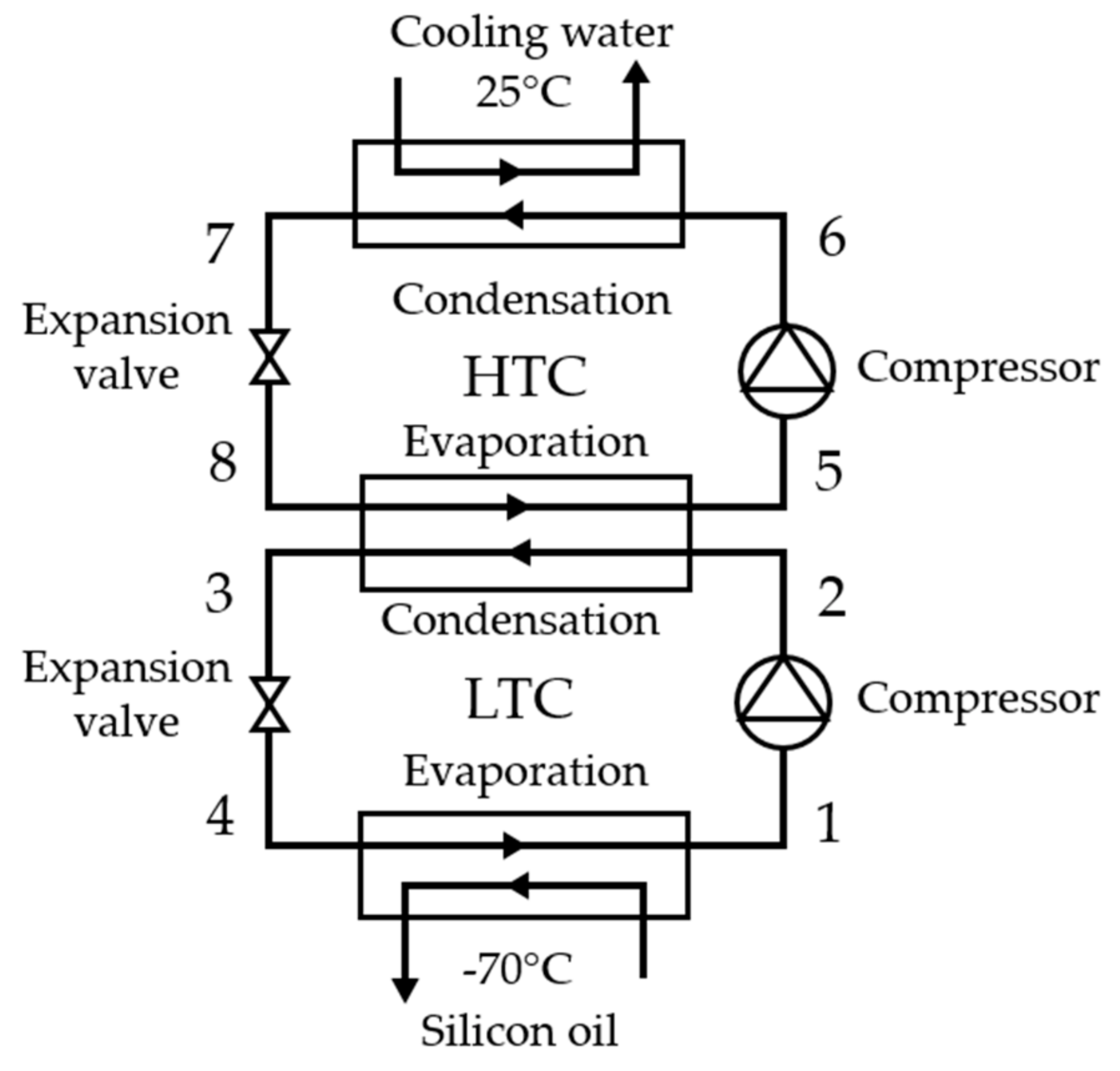
A two-stage cascade refrigeration system similar to the one installed on the pilot-scale freeze-dryer LyoBeta 25 (Telstar, Terrassa, Spain) was considered to calculate the energy consumption of the process. The cascade system works with two different refrigerants—R-404A for the high-temperature circuit (HTC) and R-23 for the low-temperature circuit (LTC)—and the two circuits are thermally connected by a cascade heat exchanger, which works as a condenser for the LTC and as an evaporator for the HTC [7], as described in Figure 1.
It is assumed that the two stages are always active, and the cycle works between TH = Tamb + 10°C and TC = Tcond – 10 °C. For simplicity in the calculations of the thermodynamic cycles, some other assumptions were made, as follows: (i) there is no superheating after evaporation, (ii) no undercooling after condensation, and (iii) the compressors work under adiabatic conditions with an isentropic efficiency . The control over the required energy is assumed to be ensured by controlling the mass flow of the refrigerant fluid circulating in the system. This latter assumption is somewhat different from the real control system present in the reference freeze-dryer, where one or both stages work depending to the temperature required, always working at maximum mass flow conditions and coupled to a heater to compensate the excess of heat removed from the system. This kind of control is more energy-consuming, and therefore our assumption is not conservative, but, unfortunately, it is impossible to model such a kind of control in a quasi-steady analysis like the one here described.
The electricity consumption of the two compressors can be expressed as
where h is the enthalpy of the refrigerant fluid at the different thermodynamic states defined as in Figure 1, and and are the total masses treated by the respective compressors.
The mass circulated in the LTC is calculated as
where is equal to the heat load to be subtracted from the system. Therefore, the mass circulated in the HTC reads:
However, an increasing number of industrial apparatus do no use compressors, but a cryogenic cooling system based on the vaporization of liquid nitrogen in a heat exchanger. In those cases, it is possible to calculate the cost of the liquid nitrogen that should be used as follows:
where is the total amount of heat that is subtracted by the cooling system, and are respectively the latent heat of boiling at atmospheric pressure and the density of liquid nitrogen, and is the cost of liquid nitrogen per cubic meter.
2.2.2. Other Electrical Consumptions
The other electrical consumptions include (i) the vacuum pump and (ii) the heat to be supplied during primary and secondary drying, and condenser defrosting. For all those terms in which heat has to be supplied by using an electric resistance, the electricity consumption can be written as:
where is the sum of all the terms in which heat has to be supplied to the system, while is the electrical efficiency that accounts for the losses in the conversion of energy in the electric resistance.
2.2.3. Operational Costs
Once everything is converted into an electrical consumption, the operational costs per cycle can be calculated easily knowing the cost of electricity, , as
2.3. Capital Costs
The capital cost per cycle, CC, can be calculated as
where is the cost of the apparatus, is the depreciation time expressed in years, is the number of working weeks in a year and is the number of cycles that can fit in a working week. is a function of the cycle duration and can be calculated in two different ways. The first option considers a working week of 7 days and, therefore, the total amount of cycles that can fit in a week is determined by dividing the number of hours in a week by the total length of a cycle. The second option considers a working week of 5 days. Moreover, it should be considered that a single cycle cannot be interrupted during the weekend, and so the number of possible cycles held in a week, , must be rounded to the lower integer.
Once all the costs per cycle are calculated, it is easy to refer them to a single vial or to a kg of dried product by just dividing the cost by the number of vials produced, or the amount of product dried in a single cycle.
2.4. Case Studies
Firstly, the model was used to evaluate the costs of a typical freeze-drying cycle and the impact of each term on the total cost. Two scenarios were compared, i.e., a laboratory pilot-scale and an industrial-scale freeze-dryer. In this comparison, the operative parameters of the process, such as temperatures, pressures, types of vials, filling volume and solid content, were the same, while the constructive parameters, such as the dimension of the chamber, the number of shelves, the number of vials, etc., for the industrial freeze-dryer were chosen to represent a possible industrial setup. The pilot-scale freeze-drier is composed of a drying chamber of 0.25 m3, with four shelves, and it can process 800 10R vials per cycle. On the other hand, the industrial scale is composed of a drying chamber of 8 m3, with 17 shelves, and it can process approximately 100,000 10R vials per cycle.
A comparison between two refrigeration methods, i.e., the typical two-stage compression refrigeration cycle and liquid nitrogen, was then made to demonstrate the necessity of working towards the development of new, greener and more affordable cooling methods.
Finally, the influence of the primary drying was evaluated more specifically to determine in which cases it is reasonable to optimize the process parameters in order to obtain a reduced primary drying duration. An interval spanning from 5 h to 40 h was evaluated, the shortest times being related to incredibly optimized cycles and stable products and the longest times being related to high-temperature sensible products and conservative process parameters.
3. Results
3.1. Operational Costs in Laboratory-Scale and Industrial Apparatus
A typical batch cycle was used to compare the operational costs of freeze-drying in a laboratory-scale apparatus and an industrial one. In this scenario, each vial 10R was filled with 3 ml of solution and frozen from 25 to −50 °C in 7 h. The primary drying stage was conducted at 10 Pa and using a shelf temperature of −20 °C, for a total duration of 28 h. The secondary drying stage was conducted at 2 Pa and a shelf temperature equal to 10 °C, for a total duration of 9 h.
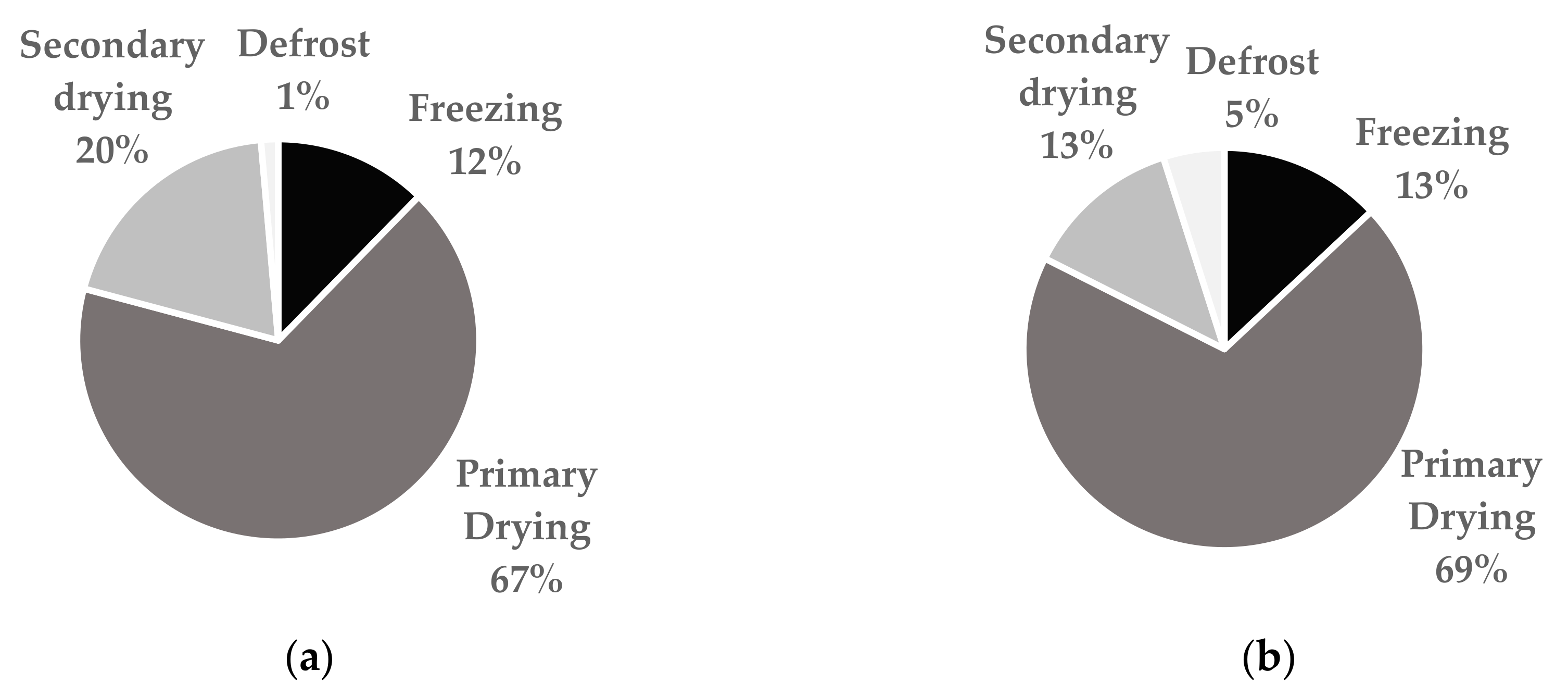
The cost of a laboratory-scale freeze-drying cycle was calculated considering typical laboratory-scale process parameters (see Appendix A). As shown in Figure 2a, 67% of the total OC is to be attributed to the primary drying, while freezing and secondary drying accounted respectively for only 12% and 20% of the total. The operational cost related to defrosting can almost be considered negligible, as it represented only 1% of the total operational cost.
Similar results were obtained for an industrial scenario, except for the defrosting, which represented 5% of the total operational costs (Figure 2b).
3.2. Operational vs. Capital Costs
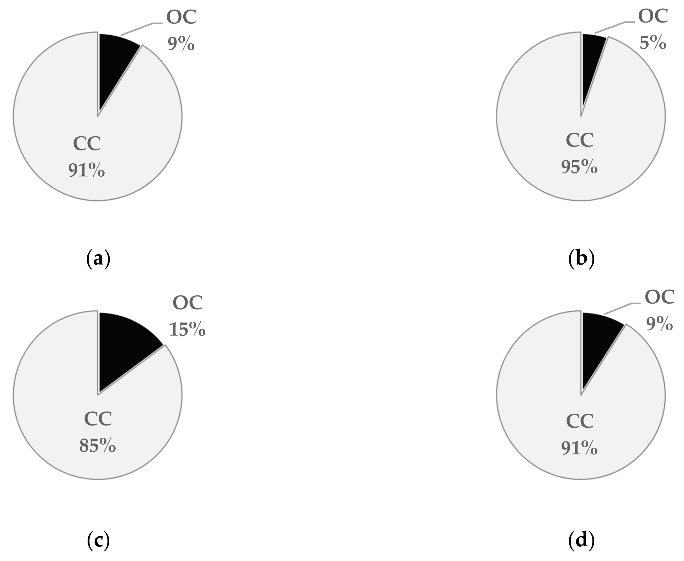
The CC per cycle was calculated, as previously described, considering two different working weeks, i.e., 7-day and 5-day working weeks. As shown in Figure 3, in both cases, the CC was shown to be much larger than the OC, these being respectively 91% and 95% of the total cost of a cycle.
It should also be noted that this result comes from a depreciation time of the freeze-dryer of 20 years, which could be greater than the common depreciation time of normal laboratory equipment, and the CC values do not consider the maintenance that is always required when a machine works for so many years. Costs related to the maintenance are scarcely documented in the literature and, therefore, it is difficult, if not impossible, to perform an estimation in such direction. The maintenance costs in industries are said to range from 15% to 40% of the total production costs [22,23,24], while in some cases peaking to 70% [25]. It is clear that those numbers can change dramatically from case to case, and as a consequence of the specific strategy of each company, and, therefore, it would be pointless to include them in the calculation. However, this result confirms that the main cost of freeze-drying is due to the raw materials and to the investments related to the machine, and not the effective utilization of the apparatus. Under these circumstances, it is possible to assume that the only reason to make any optimization in the freeze-drying cycle to reduce its total length is that more cycles would be performed in the lifespan of the freeze-dryer and, therefore, the CC would be reduced alongside with an increase in the throughput. Moreover, if the freeze-dryer works only in a 5-day working week, the correlation between the total length of the cycle and the CC is not linear. The CC per cycle is reduced only if one more cycle could fit completely in a week, and this is something that should be carefully considered when trying to reduce the costs.
Another aspect that should be taken into account, mostly for industrial plants, is the impact that Cleaning-In-Place (CIP) and Sterilization-In-Place (SIP) could have on the overall cost. Even though the literature scarcely covers this topic, the amount of water, solvents and steam that have to be used during these processes are not negligible. However, these terms were not considered in the present work because (i) the model was based on a laboratory-scale freeze-drier, and those kind of apparatus are not predisposed to such procedures, and (ii) the costs of CIP and SIP can vary significantly depending on multiple parameters, such as the dimension of the machine, the configuration, the production year. Under these circumstances, it was impossible to have a standard common value and to make any kind of comparisons. However, the reader should remember that these additional expenses must not be forgotten in future evaluations.
3.3. Manufacturing Cost per Unit Dose
The manufacturing costs were analyzed for a typical freeze-dried unit dose produced using both a pilot-scale and an industrial-scale freeze-drier; in this analysis, the costs of materials (vials, stopper, excipients and APIs) were not considered because many of these costs can drastically vary depending on the formulation, supplier or upstream route of synthesis/processes.
As shown in Table 1, the OC per cycle performed in the industrial freeze-dryer increased by a factor 30 with respect to the pilot-scale freeze-drier, while the CC increased by a factor 20. This difference is quite normal considering that the price of the machine usually grows less than linearly with the dimension of the machine itself. Moreover, our data showed that in the industrial configuration, the OC increased their relevance in the budget of the process; see Figure 3.
However, even considering this enormous increase in the costs, it is interesting to make a comparison between the costs per dose for the two configurations. Even though the total cost of a cycle for an industrial freeze-dryer is 25 times greater, the cost per dose is six times smaller because of the increase in productivity. This is clearly something expected, as the principal objective of a process scale-up is to reduce the costs and to increase productivity, and it is indeed proof that the model used in this work is robust.
3.4. Refrigeration with Liquid Nitrogen
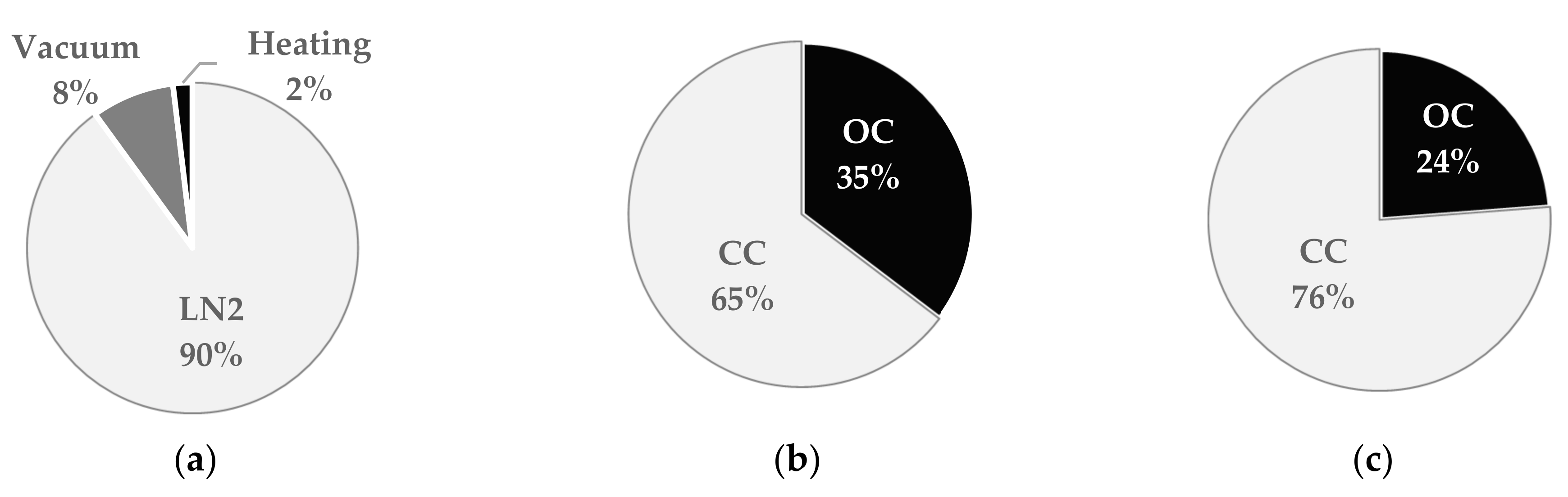
When the liquid nitrogen is used in place of a typical refrigeration cycle, the OC increased tremendously. As shown in Figure 4, the cost of the liquid nitrogen itself accounted for 90% of the OC. In this case, the OC represented 35% of the total costs of a cycle if a 7-day working week is considered, and 24% if a 5-day working week is considered.
The reason for this increase lies in the high cost of the liquid nitrogen and the fact that, at this point of the study, the cooling power of the nitrogen is not used completely. For example, it is possible to reduce the costs by reducing the amount of liquid nitrogen used in extracting the sensible heat of the cryogenic gaseous nitrogen vapor. The liquid nitrogen, at atmospheric pressure, boils at −196 °C, which means that there is a theoretical usable increase in temperature of around 200 K in the vapor if used in an integrated cooling system. With the latent heat of the fusion of liquid nitrogen being 200 times greater than the specific heat of the vapor, it is possible to reduce the cost of the nitrogen by half. Another important factor in the reduction of the nitrogen cost is its supply. In this calculation, the cost was considered as if fresh nitrogen was bought every time it was consumed. If some kind of on-site production is applied, mostly for industrial plants, the cost could drop enormously. Anyway, the aim of this work is not to optimize the use of liquid nitrogen as a cooling medium, but to demonstrate that it could be an expensive alternative to the systems currently used. However, the use of liquid nitrogen presents the advantage of not using mechanical systems, and, so, the probability of failures in the cooling systems is reduced.
In a near future, when ozone-depleting gases will not be available anymore and the industry will have to deal with the use of other technological solutions, many research laboratories and pharmaceutical plants could face unexpected expenses. Significant efforts should be made now in order to be prepared for when the change will be inevitable.
3.5. Optimization and Reduction of Primary Drying Duration
In this section, we show the benefit of cycle optimization in manufacturing costs. Here, OC, CC and total costs were calculated as a function of the primary drying duration
The main strategies for reducing the primary drying duration were:
- Control of nucleation during the freezing stage;
- Optimization of shelf temperature during primary drying.
Controlled nucleation is well known for its capability in reducing primary drying duration, but also the intra-batch heterogeneity [26,27,28,29,30,31]. This strategy consists of the trigger nucleation in the liquid solution contained in every vial of the batch at the same time, usually to higher temperatures (generally, from 0 to −10 °C) compared to those at which spontaneous nucleation occurs. Moreover, if the nucleation is not controlled, the nucleation temperature varies stochastically in every sample in a range from −5 to −40 °C, leading to high intra-batch heterogeneity and, possibly, to batch-to-batch variability. On the other hand, if the nucleation temperature is controlled, the samples present a more uniform structure, reducing the intra-batch heterogeneity but also the batch-to-batch variability. Moreover, the high nucleation temperature leads to bigger crystals and, consequently, to bigger pores in the dried cake, resulting in a sharp decrease in mass transfer resistance to vapor flow.
A second approach to reducing primary drying cycles consists of a careful optimization of the shelf temperature and chamber pressure during the process, and maximizing the heat and mass transfer [32,33,34,35]. The main constraint of this strategy lies in the maximum temperature that the product being dried cannot exceed during the process, the so-called target temperature. The target temperature is usually set between 2 and 5 °C below collapse temperature, and it is an intrinsic constraint of the formulation itself.
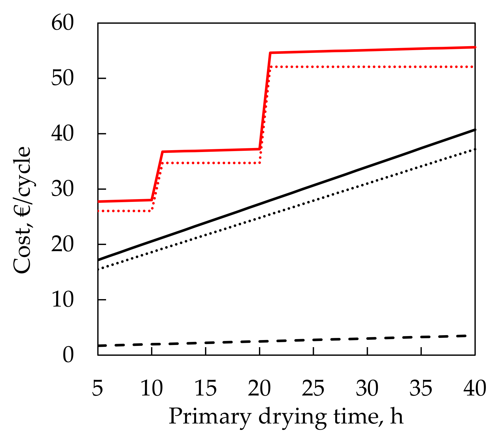
As shown in Figure 5, even though the OC increase linearly with respect to the primary drying duration, the slope is much smaller compared to CC, when calculated for a 7-day working week. When the total cost of a cycle is calculated with a 5-day working week, the total cost is obviously greater compared to the 7-day working week, and its increase is not linear anymore, but stepwise. As a matter of fact, if the freeze-dryer has to be stopped during the weekends, the number of complete cycles that can fit in a working week can increase only at specified values corresponding to those cycle lengths that allow one to fit an integer number of cycles in 5 days.
However, the duration of the primary drying cannot be reduced indefinitely, and a specific analysis should be made for each product and formulation.
4. Discussion
In this work, the operational and capital costs of a freeze-dryer were analyzed by means of a detailed mathematical model. The results obtained showed that the main cost of the process is not the utilization of the freeze-dryer, but the initial investment. When compared to the total costs of a cycle, the OC account only for 9% when a 5-day working week is considered, and for 5% in the case of a 7-day working week. In a laboratory-scale scenario, primary drying represents 67% of the total OC, while secondary drying and freezing represent 20% and 12%, respectively. The defrosting of the condenser, being roughly 1% of the OC, can be considered negligible. In the comparison between pilot- and industrial-scale, the model predicted that the cost of unit doses produced in a laboratory-scale apparatus is much higher compared to those produced in an industrial-scale freeze-dryer. This result is expected, but is indeed proof of the robustness of the model. A rough evaluation of a possible alternative process scenario was made considering the utilization of boiling liquid nitrogen as the cooling fluid for the whole system. The OC increased tremendously, becoming 35% and 24% of the total costs, respectively, for the 5-day working week and the 7-day working week, the main reason being the incredibly high cost of the liquid nitrogen. The evaluation was made necessary by the recent ban on the greenhouse gases that are now used as technological fluids for refrigeration systems. Its aim was to bring the attention of the food and pharmaceutical industry onto the urge to find other suitable alternatives in short times, as the cost of this already expensive process could ramp up to unsustainable values. Finally, an analysis of the benefits that the optimization of the primary drying time could bring was made. The results show that, due to the relatively small operational costs, the main gain of a hypothetical reduction in the primary drying time is that more cycles could fit in the working lifetime of a freeze-dryer and that, therefore, the capital costs would diminish while the productivity would increase. An improved scheduling of the cycles is, accordingly, the only reason to perform any optimization of the process. As a matter of fact, when plant breaks during the weekends are considered, significant benefits are achieved only if one more entire cycle fits in the working week. These results have never been addressed before in the literature; in fact, there are no other studies focusing on both the energetic and cost estimation. Future research should focus on the application of the model to real case studies in the industry, e.g., by performing suitable experiments for a direct comparison with the theoretical results, and on the evaluation of the possible hidden efficiencies or parameters not yet considered that should be included in the analysis. However, the hope of the authors is that this model could be used to investigate the eventual bottlenecks of the process, and to guide future research on the thoughtful optimization of the various parameters of the process.
Author Contributions
Conceptualization, methodology, data curation, L.S., S.F., L.C.C., and R.P.; writing—original draft preparation, L.S.; writing—review and editing, L.C.C. and R.P.; All authors have read and agreed to the published version of the manuscript.
Funding
This research received no external funding.
Conflicts of Interest
The authors declare no conflict of interest.
Appendix A

Table A1.
List of the variables used in this work and their numerical value.
| Variable | Laboratory Freeze-Drier | Industrial Freeze-Drier | Units |
|---|---|---|---|
| nvials/shelf | 200 | 6000 | - |
| nshelf | 4 | 17 | - |
| tF | 7 | 7 | h |
| tPD | 28 | 28 | h |
| tSD | 9 | 9 | h |
| tdead time | 4 | 4 | h |
| Tamb | 25 | 25 | °C |
| Tn | 0 | 0 | °C |
| TF | −50 | −50 | °C |
| TF,walls | −15 | −15 | °C |
| TPD | −20 | −20 | °C |
| TPD,walls | 15 | 15 | °C |
| TSD | 10 | 10 | °C |
| TSD,walls | 15 | 15 | °C |
| Tcond | −70 | −70 | °C |
| PPD | 10 | 10 | Pa |
| PSD | 2 | 2 | Pa |
| Patm | 101,325 | 101,325 | Pa |
| mprod/vial | 3 | 3 | g |
| mglass/vial | 10 | 10 | g |
| mstop/vial | 1 | 1 | g |
| cp,w | 4.186 | 4.186 | kJ/kg°C |
| cp,i | 2.090 | 2.090 | kJ/kg°C |
| cp,sol | 1.383 | 1.383 | kJ/kg°C |
| cv,air | 0.715 | 0.715 | kJ/kg°C |
| cp,glass | 0.840 | 0.840 | kJ/kg°C |
| cp,stop | 0.240 | 0.240 | kJ/kg°C |
| cp,steel | 0.502 | 0.502 | kJ/kg°C |
| cp,oil | 1.5 | 1.5 | kJ/kg°C |
| λf,w | 333.6 | 333.6 | kJ/kg |
| λsub,w | 2838.0 | 2838.0 | kJ/kg |
| λdes,w | 2687.4 | 2687.4 | kJ/kg |
| λboil,LN | 198.9 | 198.9 | kJ/kg |
| ρair | 1.4 | 1.4 | kg/m3 |
| ρsteel | 8000 | 8000 | kg/m3 |
| ρoil | 971 | 971 | kg/m3 |
| ρLN | 807 | 807 | kg/m3 |
| xw | 0.95 | 0.95 | - |
| xsol | 0.05 | 0.05 | - |
| φPD | 0.92 | 0.92 | - |
| φSD | 0.08 | 0.08 | - |
| Wch | 600 | 2000 | mm |
| Lch | 600 | 2000 | mm |
| Hch | 700 | 2000 | mm |
| swalls | 10 | 20 | mm |
| Wsh | 380 | 1300 | mm |
| Lsh | 450 | 1300 | mm |
| sshelf | 4 | 4 | mm |
| soil | 12 | 12 | mm |
| sins | 50 | 100 | mm |
| sdoor | 40 | 50 | mm |
| ksteel | 15 | 15 | W/m°C |
| kins | 0.03 | 0.03 | W/m°C |
| kdoor | 0.20 | 0.20 | W/m°C |
| hin | 5 | 5 | W/m2°C |
| hout | 20 | 20 | W/m2°C |
| PM | 3.70 | 40 | kW |
| Pn | 0.75 | 9.2 | kW |
| Vcond | 0.012 | 1 | m3 |
| pump | 20.5 | 200 | m3/h |
| ηel | 0.5 | 0.5 | - |
| ηis | 0.7 | 0.7 | - |
| h1 | 323 | 323 | kJ/kg |
| h2 | 423 | 423 | kJ/kg |
| h3 | 168 | 168 | kJ/kg |
| h4 | 168 | 168 | kJ/kg |
| h5 | 349 | 349 | kJ/kg |
| h6 | 406 | 406 | kJ/kg |
| h7 | 251 | 251 | kJ/kg |
| h8 | 251 | 251 | kJ/kg |
| tdep | 20 | 20 | y |
| nw/y | 48 | 48 | w |
| CLN | 100 | 100 | €/m3 |
| Cel | 0.06568 | 0.06568 | €/kWh |
| Cfreeze-dryer | 100 | 2000 | k€ |
References
- Rey, L. Glimpses into the Realm of Freeze-Drying: Classical Issues and New Ventures. In Freeze Drying/Lyophilization of Pharmaceuticals and Biological Products, 3rd ed.; Rey, L., May, J.C., Eds.; Informa Healthcare: London, UK, 2010; pp. 1–28. [Google Scholar]
- Oetjen, G.W.; Haseley, P.U. Freeze-Drying, 2nd ed.; John Wiley & Sons: New York, NY, USA, 2008. [Google Scholar]
- Ratti, C. Freeze-Drying Process Design. In Handbook of Food Process Design; Rahman, S., Ahmed, J., Eds.; Wiley-Blackwell: Hoboken, NJ, USA, 2012; pp. 621–647. [Google Scholar]
- Zhang, S.Z.; Luo, J.L.; Chen, G.M.; Wang, Q. Thermodynamic Analysis of a Freeze-Dryer Utilizing Hygroscopic Solution. Dry. Technol. 2018, 36, 697–708. [Google Scholar]
- Bruttini, R.; Crosser, O.K.; Liapis, A.I. Exergy Analysis for the Freezing Stage of the Freeze Drying Process. Dry. Technol. 2001, 19, 2303–2313. [Google Scholar] [CrossRef]
- Liapis, A.I.; Bruttini, R. Exergy Analysis of Freeze Drying of Pharmaceuticals in Vials on Trays. Int. J. Heat Mass Transf. 2008, 51, 3854–3868. [Google Scholar] [CrossRef]
- Renteria Gamiz, A.G.; Van Bockstal, P.J.; De Meester, S.; De Beer, T.; Corver, J.; Dewulf, J. Analysis of a pharmaceutical batch freeze dryer: Resource consumption, hotspots, and factors for potential improvement. Dry. Technol. 2019, 37, 1563–1582. [Google Scholar] [CrossRef]
- Duan, X.; Yang, X.T.; Ren, G.Y.; Pang, Y.Q.; Liu, L.L.; Liu, Y.H. Technical Aspects in Freeze-Drying of Foods. Dry. Technol. 2016, 34, 1271–1285. [Google Scholar] [CrossRef]
- Ratti, C. Hot air and freeze-drying of high-value foods: A review. J. Food Eng. 2001, 49, 311–319. [Google Scholar] [CrossRef]
- Millman, M.; Liapis, A.; Marchello, J. Note on the economics of batch freeze dryers. Int. J. Food Sci. Technol. 1985, 5, 541–551. [Google Scholar] [CrossRef]
- Bird, K. Freeze-Drying of Foods: Cost Projections; Marketing Research Report n.639; Marketing Economics Division, Economic Research Service; US Department of Agriculture: Washington, DC, USA, 1964. [Google Scholar]
- Arsiccio, A.; Giorsello, P.; Marenco, L.; Pisano, R. Considerations on Protein Stability During Freezing and Its Impact on the Freeze-Drying Cycle: A Design Space Approach. J. Pharm. Sci. 2019, 109, 464–475. [Google Scholar] [CrossRef] [Green Version]
- Arsiccio, A.; Pisano, R. Application of the Quality by Design Approach to the Freezing Step of Freeze-Drying: Building the Design Space. J. Pharm. Sci. 2018, 107, 1586–1596. [Google Scholar] [CrossRef]
- Pisano, R.; Arsiccio, A.; Nakagawa, K.; Barresi, A.A. Tuning, measurement and prediction of the impact of freezing on product morphology: A step toward improved design of freeze-drying cycles. Dry. Technol. 2019, 37, 579–599. [Google Scholar] [CrossRef]
- Oddone, I.; Arsiccio, A.; Duru, C.; Malik, K.; Ferguson, J.; Pisano, R.; Matejtschuk, P. Vacuum-Induced Surface Freezing for the Freeze-Drying of the Human Growth Hormone: How Does Nucleation Control Affect Protein Stability? J. Pharm. Sci. 2020, 109, 254–263. [Google Scholar] [CrossRef] [Green Version]
- Fissore, D.; Pisano, R. Computer-Aided Framework for the Design of Freeze-Drying Cycles: Optimization of the Operating Conditions of the Primary Drying Stage. Processes 2015, 3, 406. [Google Scholar] [CrossRef]
- Vilas, C.; Alonso, A.A.; Balsa-Canto, E.; López-Quiroga, E.; Trelea, I.C. Model-Based Real Time Operation of the Freeze-Drying Process. Processes 2020, 8, 325. [Google Scholar] [CrossRef] [Green Version]
- Vanbillemont, B.; Nicolaï, N.; Leys, L.; De Beer, T. Model-Based Optimisation and Control Strategy for the Primary Drying Phase of a Lyophilisation Process. Pharmaceutics 2020, 12, 181. [Google Scholar] [CrossRef] [PubMed] [Green Version]
- Pisano, R.; Arsiccio, A.; Capozzi, L.C.; Trout, B.L. Achieving continuous manufacturing in lyophilization: Technologies and approaches. Eur. J. Pharm. Biopharm. 2019, 142, 265–279. [Google Scholar] [CrossRef]
- Adali, M.B.; Barresi, A.A.; Boccardo, G.; Pisano, R. Spray Freeze-Drying as a Solution to Continuous Manufacturing of Pharmaceutical Products in Bulk. Processes 2020, 8, 709. [Google Scholar] [CrossRef]
- Pisano, R. Continuous manufacturing of lyophilized products: Why and how to make it happen. Am. Pharm. Rev. 2020, 23, 20–22. [Google Scholar]
- Maggard, B.N.; Rhyne, D.M. Total productive maintenance. A timely integration of production and maintenance. Prod. Inventory Manag. J. 1992, 33, 6–10. [Google Scholar]
- Löfsten, H. Measuring maintenance performance—In search for a maintenance productivity index. Int. J. Prod. Econ. 2000, 63, 47–58. [Google Scholar] [CrossRef]
- Vishnu, C.R.; Regikumar, V. Reliability Based Maintenance Strategy Selection in Process Plants: A Case Study. Proc. Technol. 2016, 25, 1080–1087. [Google Scholar] [CrossRef] [Green Version]
- Bevilacqua, M.; Braglia, M. The analytic hierarchy process applied to maintenance strategy selection. Reliab. Eng. Syst. Saf. 2000, 70, 71–83. [Google Scholar] [CrossRef]
- Kochs, M.; Körber, C.; Nunner, B.; Heschel, I. The influence of the freezing process on vapour transport during sublimation in vacuum-freeze-drying. Int. J. Heat Mass Transf. 1991, 34, 2395–2408. [Google Scholar] [CrossRef]
- Searles, J.A.; Carpenter, J.F.; Randolph, T.W. The Ice Nucleation Temperature Determines the Primary Drying Rate of Lyophilization for Samples Frozen on a Temperature-Controlled Shelf. J. Pharm. Sci. 2001, 90, 860–871. [Google Scholar] [CrossRef]
- Hottot, A.; Vessot, S.; Andrieu, J. Freeze drying of pharmaceuticals in vials: Influence of freezing protocol and sample configuration on ice morphology and freeze-dried cake texture. Chem. Eng. Process. 2007, 46, 666–674. [Google Scholar] [CrossRef]
- Kasper, J.C.; Friess, W. The freezing step in lyophilisation: Physico-chemical fundamentals, freezing methods and consequences on process performance and quality attributes of biopharmaceuticals. Eur. J. Pharm. Biopharm. 2011, 78, 248–263. [Google Scholar] [CrossRef] [PubMed]
- Arsiccio, A.; Matejtschuk, P.; Ezeajughi, E.; Riches-Duit, A.; Bullen, A.; Malik, K.; Raut, S.; Pisano, R. Impact of controlled vacuum induced surface freezing on the freeze drying of human plasma. Int. J. Pharm. 2020, 582, 119290. [Google Scholar] [CrossRef]
- Arsiccio, A.; Barresi, A.; De Beer, T.; Oddone, I.; Van Bockstal, P.J.; Pisano, R. Vacuum Induced Surface Freezing as an effective method for improved inter- and intra-vial product homogeneity. Eur. J. Pharm. Biopharm. 2018, 128, 210–219. [Google Scholar] [CrossRef] [PubMed]
- Pisano, R.; Fissore, D.; Barresi, A. Freeze-Drying Cycle Optimization Using Model Predictive Control Techniques. Ind. Eng. Chem. Res. 2011, 50, 7363–7379. [Google Scholar] [CrossRef]
- Fissore, D.; Pisano, R.; Barresi, A. Advanced Approach to Build the Design Space for the Primary Drying of a Pharmaceutical Freeze-Drying Process. J. Pharm. Sci. 2011, 100, 4922–4933. [Google Scholar] [CrossRef]
- Fissore, D.; Pisano, R.; Barresi, A. Applying quality-by-design to develop a coffee freeze-drying process. J. Food Eng. 2014, 123, 179–187. [Google Scholar] [CrossRef] [Green Version]
- Pikal, M.J.; Shah, S.; Roy, M.L.; Putman, R. The secondary drying of freeze-drying: Drying kinetics as a function of the temperature and chamber pressure. Int. J. Pharm. 1990, 60, 203–217. [Google Scholar] [CrossRef]
Figure 1.
Scheme of the two-stages refrigeration cycle considered for the calculation of the power consumption attributed to the refrigeration system. The numbers refer to the thermodynamics states of the refrigerant fluids.
Figure 1.
Scheme of the two-stages refrigeration cycle considered for the calculation of the power consumption attributed to the refrigeration system. The numbers refer to the thermodynamics states of the refrigerant fluids.

Figure 2.
Percentage distribution of the operational costs (OC) of the fundamental steps of a lyophilization cycle for (a) a laboratory freeze-dryer and (b) an industrial freeze-dryer.
Figure 2.
Percentage distribution of the operational costs (OC) of the fundamental steps of a lyophilization cycle for (a) a laboratory freeze-dryer and (b) an industrial freeze-dryer.

Figure 3.
Distribution of the operational costs (OC) and capital costs (CC) for a laboratory (a,b) and an industrial (c,d) freeze-dryer. The capital costs were calculated in this work considering a 7-day working week (a,c) in which there are no interruptions in the production and a 5-day working week (b,d) that accounts for plant stops during the weekends.

Figure 4.
Operational costs and capital costs distributions calculated for the scenario in which the liquid nitrogen is used as a cooling source. In (a) the OC can be seen as divided into the three main categories that are cooling, heating and vacuum production. In (b) and (c), the ratio between OC and CC is shown. The capital costs were calculated considering a 7-day working week (b) in which there are no interruptions in the production, and a 5-day working week (c) that accounts for plant stops during the weekends.

Figure 5.
Evolution of the costs of a freeze-drying cycle conducted with a laboratory lyophilizer. It is possible to see how the operational costs (black dashed line) consist of a small fraction of the capital costs, calculated when considering either a 7-day (black dotted line) or a 5-day (red dotted line) working week. The total costs (solid lines) reflect, therefore, the behavior of the capital costs.

Table 1.
Operational (OC) and capital (CC) costs comparison for a laboratory and an industrial freeze-dryer.
Table 1.
Operational (OC) and capital (CC) costs comparison for a laboratory and an industrial freeze-dryer.
| Freeze-Dryer | OC, €/cycle | CC, €/cycle | Total Cost, €/cycle | Total Cost, €/dose |
|---|---|---|---|---|
| Laboratory | 3.28 | 29.76 | 33.04 | 0.041 |
| Industrial | 107.27 | 595.24 | 702.51 | 0.007 |
Publisher’s Note: MDPI stays neutral with regard to jurisdictional claims in published maps and institutional affiliations. |
© 2020 by the authors. Licensee MDPI, Basel, Switzerland. This article is an open access article distributed under the terms and conditions of the Creative Commons Attribution (CC BY) license (http://creativecommons.org/licenses/by/4.0/).
Share and Cite
MDPI and ACS Style
Stratta, L.; Capozzi, L.C.; Franzino, S.; Pisano, R. Economic Analysis of a Freeze-Drying Cycle. Processes 2020, 8, 1399. https://doi.org/10.3390/pr8111399
AMA Style
Stratta L, Capozzi LC, Franzino S, Pisano R. Economic Analysis of a Freeze-Drying Cycle. Processes. 2020; 8(11):1399. https://doi.org/10.3390/pr8111399
Chicago/Turabian StyleStratta, Lorenzo, Luigi C. Capozzi, Simone Franzino, and Roberto Pisano. 2020. "Economic Analysis of a Freeze-Drying Cycle" Processes 8, no. 11: 1399. https://doi.org/10.3390/pr8111399
Note that from the first issue of 2016, this journal uses article numbers instead of page numbers. See further details here.