1. Introduction
Prostate cancer is the most frequently diagnosed cancer in men aside from skin cancer, and 180,890 new cases of prostate cancer have been expected in the US during 2016 [
1,
2]. The only well-established risk factors for prostate cancer are increasing age, a family history of the disease, and genetic conditions. Prostate imaging is still a critical and challenging issue in diagnosis, therapy, and staging of prostate cancer (PCa). Using different imaging modalities, such as Transrectal Ultrasound (TRUS), Computed Tomography (CT) or Magnetic Resonance Imaging (MRI), is dependent on the clinical context. Currently, high-resolution multiparametric MRI has been shown to have higher accuracy than TRUS when used to ascertain the presence of prostate cancer [
3]. In [
4], MRI-guided biopsy showed a high detection rate of clinically significant PCa in patients with persisting cancer suspicion, also after a previous negative systematic TRUS-guided biopsy, which represents the gold-standard for diagnosis of prostate cancer [
5]. In addition, MRI scanning before a biopsy can also serve as a triage test in men with raised serum Prostate-Specific Antigen (PSA) levels, in order to select those for biopsy with significant cancer that requires treatment [
6]. For instance, PCa treatment by radiotherapy requires an accurate localization of the prostate. In addition, neighboring tissues and organs at risk, i.e., rectum and bladder, must be carefully preserved from radiation, whereas the tumor should receive a prescribed dose [
7]. CT has been traditionally used for radiotherapy treatment planning, but MRI is rapidly gaining relevance because of its superior soft tissue contrast, especially in conformal and intensity-modulated radiation therapy [
8].
Manual detection and segmentation of both prostate gland and prostate carcinoma on multispectral MRI is a time-consuming task, which has to be performed by experienced radiologists [
9]. In fact, in addition to conventional structural T1-weighted (T1w) and T2-weighted (T2w) MRI protocols, complementary and powerful functional information about the tumor can be extracted [
10,
11,
12] from: Dynamic Contrast Enhanced (DCE) [
13], Diffusion Weighted Imaging (DWI) [
14], and Magnetic Resonance Spectroscopic Imaging (MRSI) [
15,
16]. A standardized interpretation of multiparametric MRI is very difficult and significant inter-observer variability has been reported in the literature [
17]. The increasing number and complexity of multispectral MRI sequences could overwhelm analytic capabilities of radiologists in their decision-making processes. Therefore, automated and computer-aided segmentation methods are needed to ensure result repeatability.
Accurate prostate segmentation on different imaging modalities is a mandatory step in clinical activities. For instance, prostate boundaries are used in several treatments of prostate diseases: radiation therapy, brachytherapy, High Intensity Focused Ultrasound (HIFU) ablation, cryotherapy, and transurethral microwave therapy [
10]. Prostate volume, which can be directly calculated from the prostate Region of Interest (ROI) segmentation, aids in diagnosis of benign prostate hyperplasia and prostate bulging. Precise prostate volume estimation is useful for calculating PSA density and for evaluating post-treatment response. However, these tasks require several degrees of manual intervention, and may not always yield accurate estimates [
18]. From a computer science perspective, especially in automatic MR image analysis for prostate cancer segmentation and characterization, the computed prostate ROI is very useful for the subsequent more advanced processing steps [
12].
Despite the technological developments in MRI scanners and coils, prostate images are prone to artifacts related to magnetic susceptibility. Although the transition from 1.5 Tesla to 3 Tesla magnetic field strength systems theoretically results in a doubled Signal to Noise Ratio (SNR), it also involves different T1 (spin-lattice) and T2 (spin-spin) relaxation times and greater magnetic field inhomogeneity in the organs and tissues of interest [
19,
20]. On the other hand, 3 Tesla MRI scanners allow using pelvic coils instead of endorectal coils, obtaining good quality images and avoiding invasiveness as well as prostate gland compression and deformation. Thus, challenges for automatic segmentation of the prostate in MR images include the presence of imaging artifacts due to air in the rectum (i.e., susceptibility artifacts) and large intensity inhomogeneities of the magnetic field (i.e., streaking or shadowing artifacts), the large anatomical variability between subjects, the differences in rectum and bladder filling, and the lack of a normalized “Hounsfield unit” for MRI, like in CT scans [
7].
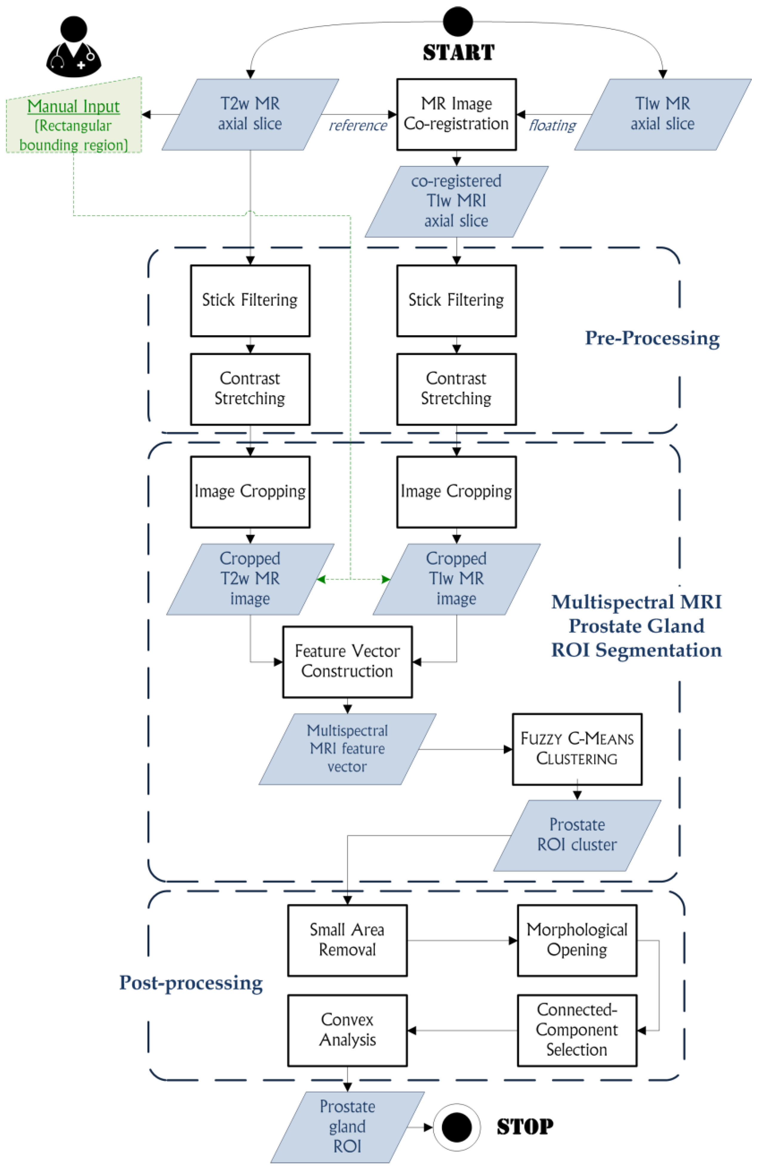
In this paper, an automated segmentation method, based on the
Fuzzy C-Means (FCM) clustering algorithm [
21], for multispectral MRI morphologic data processing is proposed. This approach allows for prostate segmentation and automatic gland volume calculation. The clustering procedure is performed on co-registered T1w and T2w MR image series. This unsupervised Machine Learning technique, by exploiting a flexible fuzzy model to integrate different MRI sequences, is able to achieve accurate and reliable segmentation results. To the best of our knowledge, this is the first work combining T1w and T2w MR image information to enhance prostate gland segmentation, by taking advantage of the uniform gray appearance of the prostate on T1w MRI, as described in [
22]. Segmentation tests were performed on an MRI dataset composed of 21 patients with suspicion of PCa, using volume-based, spatial overlap-based and spatial distance-based metrics to evaluate the effectiveness and the clinical feasibility of the proposed approach.
The structure of the manuscript is the following:
Section 2 introduces the background about MRI prostate segmentation methods,
Section 3 reports the analyzed multispectral MRI anatomical data and describes the proposed prostate gland segmentation method and the used evaluation metrics,
Section 4 illustrates the achieved experimental results, Finally, some discussions and conclusions are provided in
Section 5 and
Section 6, respectively.
2. Background
This Section summarizes the most representative literature works on prostate segmentation in MRI.
Klein et al. [
7] presented an automatic method, based on non-rigid registration of a set of pre-labeled atlas images, for delineating the prostate in 3D MR scans. Each atlas image is non-rigidly registered, employing Localized Mutual Information (LMI) as similarity measure [
23], with the target patient image. The registration is performed in two steps: (i) coarse alignment of the two images by a rigid registration; and (ii) fine non-rigid registration, using a coordinate transformation that is parameterized by cubic B-splines [
24]. The registration stage yields a set of transformations that can be applied to the atlas label images, resulting in a set of deformed label images that must be combined into a single segmentation of the patient image, considering majority voting (VOTE) and “Simultaneous Truth and Performance Level Estimation” (STAPLE) [
25]. The method was evaluated on 50 clinical scans (probably T2w images, but the acquisition protocol is not explicitly reported in the paper), which had been manually segmented by three experts. The Dice Similarity Coefficient (
DSC), to quantify the overlap between the automatic and manual segmentations, and the shortest Euclidean distance, between the manual and automatic segmentation boundaries, were computed. The differences among the four used fusion methods are small and mostly not statistically significant. For most test images, the accuracy of the automatic segmentation method was, on a large part of the prostate surface, close to the level of inter-observer variability. With the best parameter setting, a median
DSC of around 0.85 was achieved. The segmentation quality is especially good at the prostate-rectum interface, whereas most serious errors occurred around the tips of the seminal vesicles and at the anterior side of the prostate.
Vincent et al. in [
26] proposed a fully automatic model-based system for segmenting the prostate in MR images. The segmentation method is based on Active Appearance Models (AAMs) [
27] built from 50 manually segmented examples provided by the Medical Image Computing and Computer-Assisted Intervention (MICCAI) 2012 Prostate MR Image Segmentation 2012 (PROMISE12) team [
28]. High quality correspondences for the model are generated using a variant of the Minimum Description Length approach to Groupwise Image Registration (MDL-GIR) [
29], which finds the set of deformations for registering all the images together as efficiently as possible. A multi-start optimization scheme is used to robustly match the model to new images. To test the performance of the algorithm,
DSC, mean absolute distance and the 95th-percentile Hausdorff distance (
HD) were calculated. The model was evaluated using a Leave-One-Out Cross Validation (LOOCV) on the training data obtaining a good degree of accuracy and successfully segmented all the test data. The system was used also to segment 30 test cases (without reference segmentations), considering the results very similar to the LOOCV experiment by a visual assessment.
In [
30], a unified shape-based framework to extract the prostate from MR images was proposed. First, the authors address the registration problem by representing the shapes of a training set as point clouds. In this way, they are able to exploit the more global aspects of registration via a particle filtering based scheme [
31]. In addition, once the shapes have been registered, a cost functional is designed to incorporate both the local image statistics and the learned shape prior (used as constrain to perform the segmentation task). Satisfying experimental results were obtained on several challenging clinical datasets, considering
DSC and the 95th-percentile
HD, also compared to [
32], which employs the Chan-Vese Level Set model [
33] assuming a bimodal image.
Martin et al. [
34] presented the preliminary results of a semi-automatic approach for prostate segmentation of MR images that aims to be integrated into a navigation system for prostate brachytherapy. The method is based on the registration of an anatomical atlas computed from a population of 18 MRI studies along with each input patient image. A hybrid registration framework, which combines an intensity-based registration [
35] and a Robust Point-Matching (RPM) algorithm introducing a geometric constraint (i.e., the distance between the two point sets) [
36], is used for both atlas building and atlas registration. This approach incorporates statistical shape information to improve and regularize the quality of the resulting segmentations, using Active Shape Models (ASMs) [
37]. The method was validated on the same dataset used for atlas construction, using the LOOCV. Better segmentation accuracy, in terms of volume-based and distance-based metrics, was obtained in the apex zone and in the central zone with respect to the base of the prostate. The same authors proposed a fully automatic algorithm for the segmentation of the prostate in 3D MR images [
38]. The approach requires the use of a probabilistic anatomical atlas that is built by computing transformation fields (mapping a set of manually segmented images to a common reference), which are then applied to the manually segmented structures of the training set in order to get a probabilistic map on the atlas. The segmentation procedure is composed of two phases: (i) the processed image is registered to the probabilistic atlas and then a probabilistic segmentation (allowing the introduction of a spatial constraint) is performed by aligning the probabilistic map of the atlas against the patient’s anatomy; and (ii) a deformable surface evolves towards the prostate boundaries by merging information coming from the probabilistic segmentation, an image feature model, and a statistical shape model. During the evolution of the surface, the probabilistic segmentation allows for the introduction of a spatial constraint that prevents the deformable surface from leaking in an unlikely configuration. This method was evaluated on 36 MRI exams. The results showed that introducing a spatial constraint increases the segmentation robustness of the deformable model compared to another one that is only driven by an image appearance model.
Toth et al. [
18] used a Multifeature Active Shape (MFA) model [
39], which extends ASMs by training the multiple features for each voxel using a Gaussian Mixture Model (GMM) based on the log-likelihood maximization scheme, for estimating prostate volume from T2w MRI. Using a set of training images, the MFA learns the most discriminating statistical texture descriptors of the prostate boundary via a forward feature selection algorithm. After the identification of the optimal image features, the MFA is deformed to accurately fit the prostate border. The MFA-based volume estimation scheme was evaluated on a total 45 T2w in vivo MRI studies, corresponding to both 1.5 Tesla and 3.0 Tesla field strengths. A correlation with the ground truth volume estimations showed that the MFA had higher Pearson’s correlation coefficient values with respect to the current clinical volume estimation schemes, such as ellipsoid, Myschetzky, and prolate spheroid methodologies. In [
40], the same research team proposed a scheme to automatically initialize an ASM for prostate segmentation on endorectal in vivo multiprotocol MRI, exploiting MRSI data and identifying the MRI spectra that lie within the prostate. In fact, MRSI is able to measure relative metabolic concentrations and the metavoxels near the prostate have distinct spectral signals from metavoxels outside the prostate. A replicated clustering scheme is employed to distinguish prostatic from extra-prostatic MR spectra in the midgland. The detected spatial locations of the prostate are then used to initialize a multifeature ASM, which employs also statistical texture features in addition to intensity information. This scheme was quantitatively compared with another ASM initialization method for TRUS imaging by Cosìo [
41], showing superior average segmentation performance on 388 2D MRI sections obtained from 32 3D endorectal in vivo patient studies.
Other segmentation approaches are also able to segment the zonal anatomy of the prostate [
22], differentiating the central gland from the peripheral zone [
42]. The method in [
43] is based on a modified version of the
Evidential C-Means (ECM) clustering algorithm [
44], introducing spatial neighborhood information. A priori knowledge of the prostate zonal morphology was modeled as a geometric criterion and used as an additional data source to enhance the differentiation of the two zones. Thirty-one clinical MRI series were used to validate the accuracy of the method, taking into account interobserver variability. The mean
DSC was 89% for the central gland and 80% for the peripheral zone, calculated against an expert radiologist segmentation.
Litjens et al. [
45] proposed a zonal prostate segmentation approach based on Pattern Recognition techniques. First, they use the multi-atlas segmentation approach in [
7] for prostate segmentation, by extending it for using multi-parametric data. T2w MR images and the quantitative Apparent Diffusion Coefficient (ADC) maps were registered simultaneously, In Fact, the ADC map contains additional information on the zonal distribution within the prostate in order to differentiate between the central gland and peripheral zone. Then, for the voxel classification, the authors determined a set of features that represent the difference between the two zones, by considering three categories: anatomy (positional), intensity and texture. This voxel classification approach was validated on 48 multiparametric MRI studies with manual segmentations of the whole prostate.
DSC and Jaccard index (
JI) showed good results in zonal segmentation of the prostate and outperformed the multiparametric multi-atlas based method in [
43] in segmenting both central gland and peripheral zone.
A novel effective method, based on the
Fuzzy C-Means (FCM) algorithm [
21], is presented in this paper. This soft computing approach is more flexible than the traditional hard clustering version [
46]. Differently to the state of the art approaches, this unsupervised Machine Learning technique does not require training phases, statistical shape priors or atlas pre-labeling. Therefore, our method could be easily integrated in clinical practice to support radiologists in their daily decision-making tasks.
Another key novelty is the introduction of T1w MRI in the feature vector, composed of the co-registered T1w and T2w MR image series, fed to the proposed processing pipeline. Although T1w MR images were used in [
47] for prostate radiotherapy planning, the authors did not combine both multispectral T2w and T1w MR images using a fusion approach. Their study just highlighted that the Clinical Target Volume (CTV) segmentation results on the T1w and T2w acquisition sequences did not differ significantly in terms of manual CTV. Our work aims to show that the early integration of T2w and T1w MR image structural information significantly enhances prostate gland segmentation by exploiting the uniform gray appearance of the prostate on T1w MRI [
22].
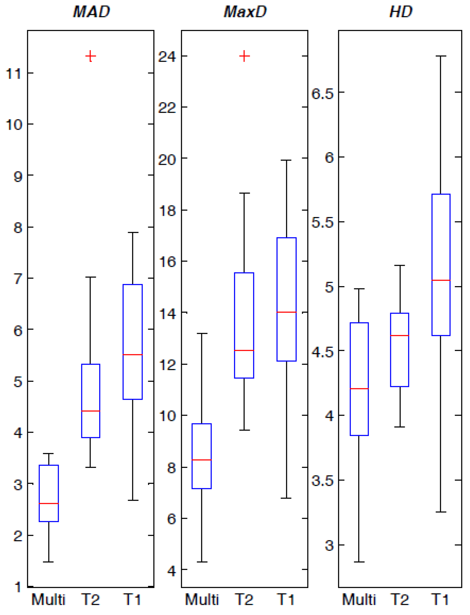
5. Discussion
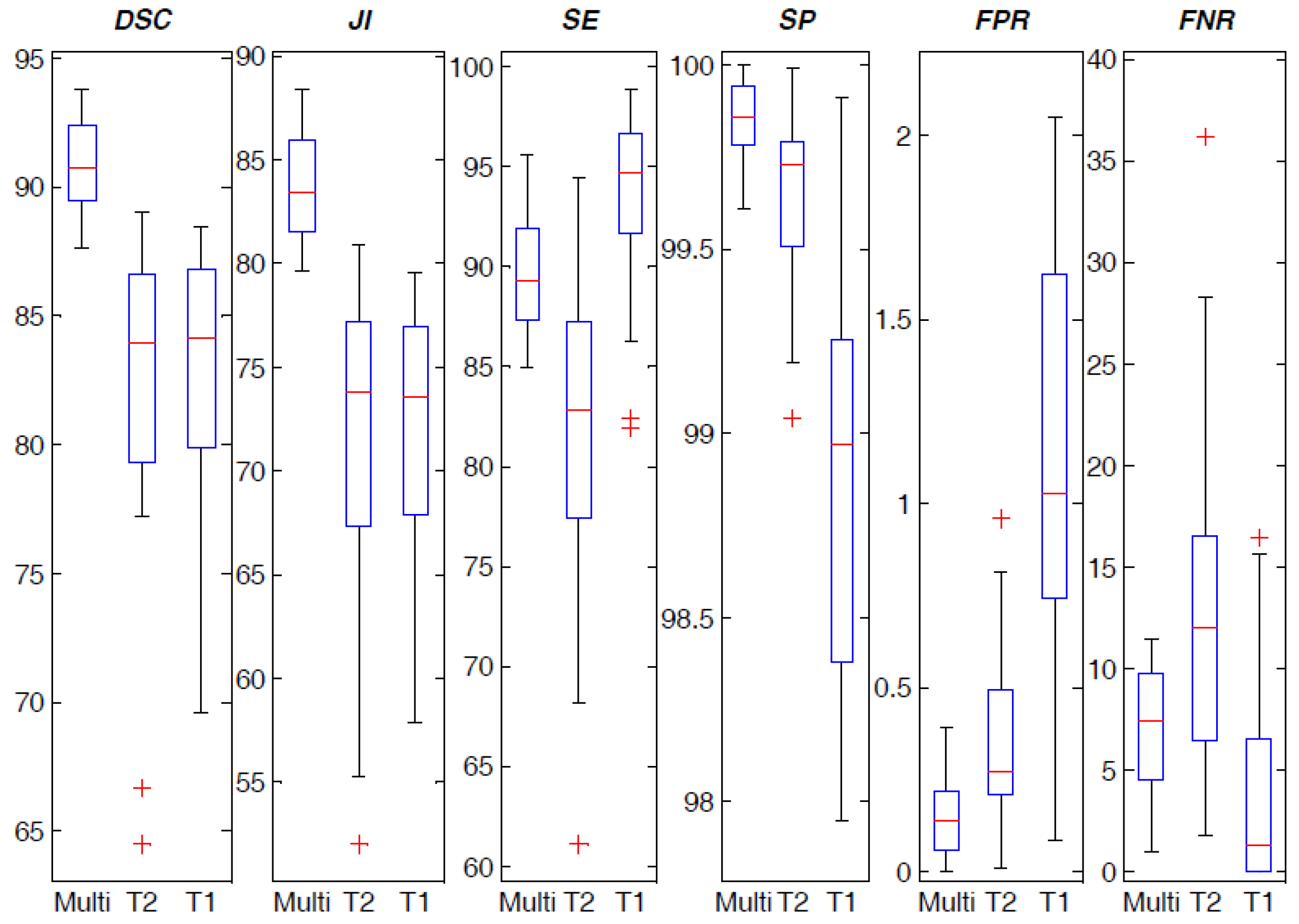
The proposed approach has proven to give good segmentation results compared to the gold-standard boundaries delineated by an experienced radiologist, as illustrated by the metrics reported in
Section 4. Although volume-based metrics do not take into account the intersection, they represent a first and immediate measure of segmentation effectiveness. Just small differences between the automatic and the manual volume measurements were observed, showing the reliability of the proposed segmentation approach for automatic volume calculation in clinical applications. The achieved overlap-based indices, which are characterized by high average values and very low standard deviation, prove the segmentation accuracy, involving the correct detection of the “true” pathological areas as well as the capability of not detecting wrong parts within the segmented prostate. The achieved spatial distance-based metrics agree with the overlap-based ones, corroborating the aforementioned experimental evidences.
The proposed method is based on an unsupervised Machine Learning technique, without requiring any training phase. On the contrary, the other literature works use or combine atlases [
7,
34,
38,
45], AAMs [
26], or statistical shape priors and ASMs [
18,
30,
34,
38,
40], which require manual labeling of a significant image sample set performed by expert physicians. In addition, as stated in [
38], atlas-based approaches may be affected by serious errors when the processed prostate instances are dissimilar to the atlas, despite the non-rigid registration.
Literature approaches used T2w MR anatomical images, sometimes combined with ADC maps [
45] or MRSI data [
40]. Our method integrated T1w and T2w MRI anatomical data to enhance clustering segmentation results. To the best of our knowledge, we combined T1w and T2w MR image series for the first time in prostate gland segmentation. As it is stated in [
12], the available public prostate MRI datasets for prostate gland segmentation and prostate cancer detection and delineation, such as PROMISE12 [
28] and the benchmark proposed in [
12], do not provide T1w MR images. Therefore, our method cannot be applied on these public datasets and compared with the prostate MR image segmentation approaches presented at the MICCAI 2012 PROMISE12 challenge, since our aim is to show that concatenating T2w and T1w pixels during the construction of the feature vector in an early integration phase. Although a comparison with state-of-the-art methods could be certainly interesting, it is also unfeasible because atlases should be built and supervised methods with a priori knowledge (such as Active Appearance Models or statistical shape priors) should be trained on our prostate MRI dataset composed of 21 patients. The number of samples is not sufficiently significant to apply suitably supervised Machine Learning techniques or shape-based models without using Leave-One-Out Cross Validation, such as in [
26,
34].
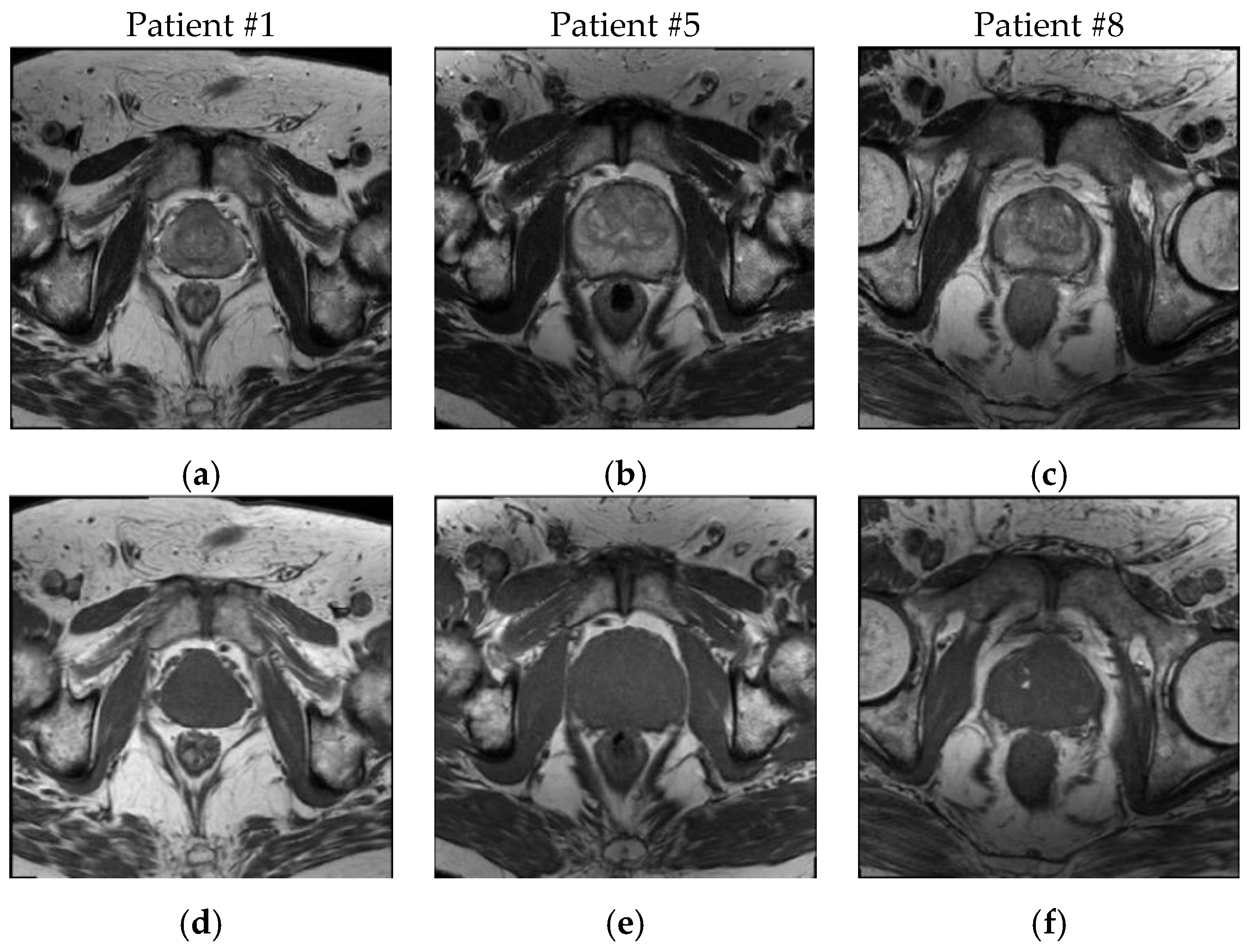
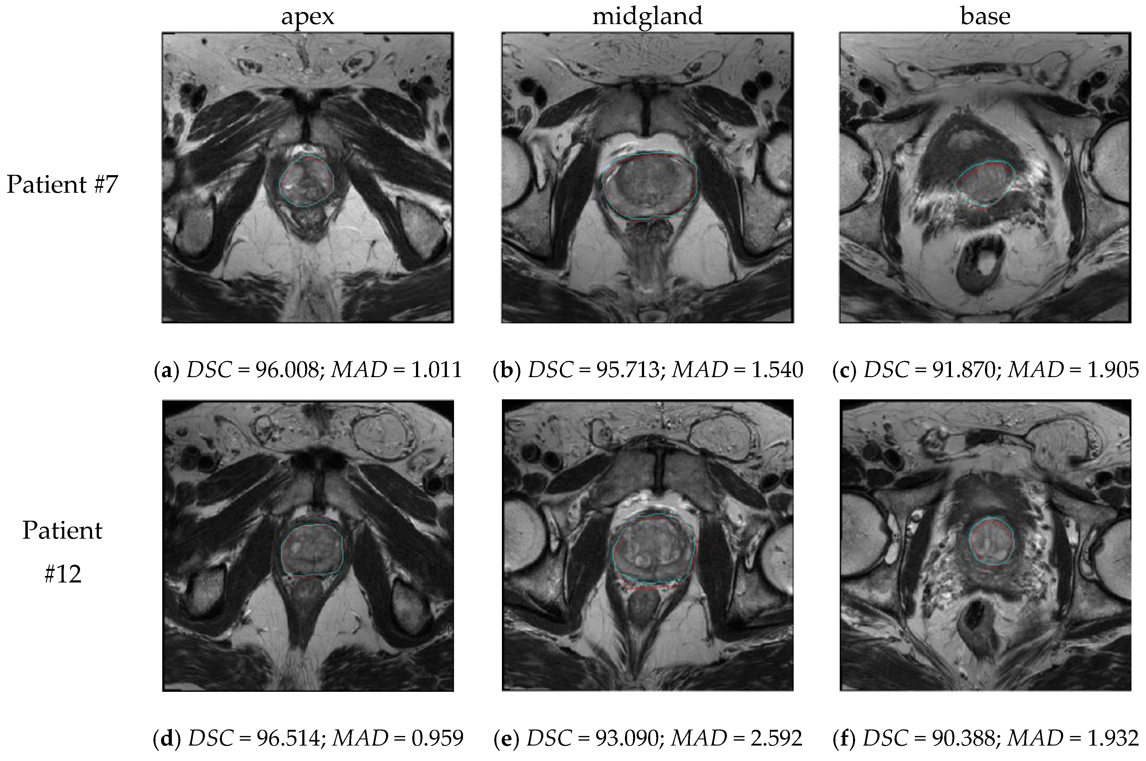
As shown in
Figure 6, our approach is also able to correctly segment apical and basal prostate MRI slices, by differentiating also seminal vesicles (see
Figure 6f). The segmentation quality was also good at the prostate-rectum and prostate-bladder interfaces. Whereas a segmentation error of a few millimeters is clinically acceptable at boundaries with muscular tissue, the interfaces with rectum and bladder need to be detected and distinguished very accurately [
7]. Moreover, good performances were obtained also with prostate glands imaged as heterogeneous regions (i.e., inhomogeneous signal in the peripheral zone or adenomatous central gland).
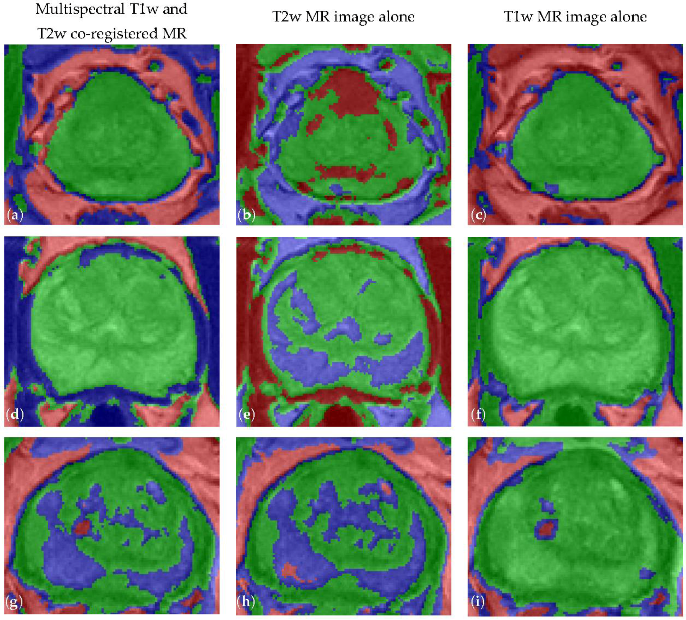
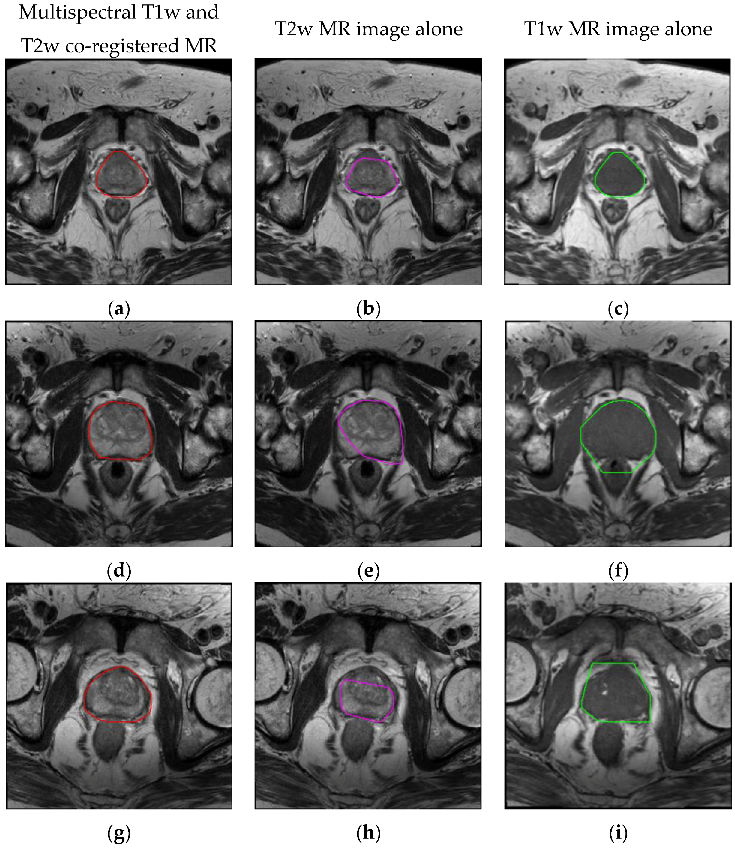
The principal experimental finding is that the
FCM clustering on multispectral MRI anatomical data considerably enhances the achieved prostate ROI segmentations, by taking advantage of the prostate uniform intermediate signal intensity at T1w imaging [
22]. The
FCM clustering algorithm on multispectral MR anatomical images allows for more accurate prostate gland ROI segmentation with respect to the clustering results on either T2w or T1w images alone. However, T1w images are often not able to distinguish among different soft tissues. For instance,
FCM clustering on T1w images alone is not able to differentiate the prostate-rectum (
Figure 5f) or the prostate-muscle (
Figure 5i) interfaces. In conclusion, combining and fusing T2w and T1w MRI data, in the feature vector construction step, allow achieving better clustering outputs.
The method was insensitive to variations in patient age, prostate volume and the presence of tumors (i.e., suspicion of cancer in different prostate regions, inhomogeneous signal in the peripheral zone or adenomatous central gland with possible nodules), also considering radiotherapy or chemotherapy treatments, thus increasing its feasibility in clinical practice.


 ,
, 


