The Effect of the Axial Heat Transfer on Space Charge Accumulation Phenomena in HVDC Cables


L.E.PR.E. HV Laboratory, Dipartimento di Ingegneria–Università di Palermo, Viale delle Scienze, Edificio 9, 90135 Palermo, Italy
*
Author to whom correspondence should be addressed.
Energies 2020, 13(18), 4827; https://doi.org/10.3390/en13184827
Submission received: 5 August 2020
/
Revised: 5 September 2020
/
Accepted: 11 September 2020
/
Published: 15 September 2020
(This article belongs to the Special Issue DC and AC Insulated Power Cables and Hybrid Transmission Lines: Insights, Operating Experiences and New Challenges)
Abstract
:To date, it has been widespread accepted that the presence of space charge within the dielectric of high voltage direct current (HVDC) cables is one of the most relevant issues that limits the growing diffusion of this technology and its use at higher voltages. One of the reasons that leads to the establishment of space charge within the insulation of cables is the temperature dependence of its conductivity. Many researchers have demonstrated that high temperature drop over the insulation layer can lead to the reversal of the electric field profile. In certain conditions, this can over-stress the insulation during polarity reversal (PR) and transient over voltages (TOV) events accelerating the ageing of the dielectric material. However, the reference standards for the thermal rating of cables are mainly thought for alternating current (AC) cables and do not adequately take into account the effects related to high thermal drops over the insulation. In particular, the difference in temperature between the inner and the outer surfaces of the dielectric can be amplified during load transients or near sections with axially varying external thermal conditions. For the reasons above, this research aims to demonstrate how much the existence of “hot points” in terms of temperature drop can weaken the tightness of an HVDC transmission line. In order to investigate these phenomena, a two-dimensional numerical model has been implemented in time domain. The results obtained for some case studies demonstrate that the maximum electric field within the dielectric of an HVDC cable can be significantly increased in correspondence with variations along the axis of the external heat exchange conditions and/or during load transients. This study can be further developed in order to take into account the combined effect of the described phenomena with other sources of introduction, forming, and accumulation of space charge inside the dielectric layer of HVDC cables.
1. Introduction
To date, the demand of high voltage direct current (HVDC) cables is growing due to the tendency to increase the amount of electric energy exchanged over long distances. Old HVDC cables with mass impregnated insulation are being replaced with extruded cables resistant to higher temperatures and with better mechanical properties. The achievement of higher temperatures leads to an increase in the ampacity of a cable, reducing the specific costs of transmission lines, but, at the same time, some collateral effects are catalyzed. In particular, the rise of Joule losses inside the conductor causes an increase in the temperature drop over the dielectric layer. As a result, this leads to an increase in the secondary mechanical stresses and to a radial variation in the electrical conductivity of the insulation. Indeed, in polymeric materials, this quantity grows exponentially with the temperature.
As widely demonstrated by many studies, in the insulation of a cable, the simultaneous existence of an electric field and a gradient in conductivity leads to a non-zero divergence of the current and therefore to the presence of space charge [1,2,3]. For the main commercial materials used as insulation for HVDC cables, it can be asserted that as the radial thermal gradient increases, the higher the electric field is close to the interface with the outer semicon, the lower the one near the interface with the inner semicon. In some cases, the electric field at the external boundary of the insulation layer of a loaded cable can exceed its value at the inner boundary reached in no-load conditions. This scenario is more likely to occur in large cables loaded with rated current or under emergency load conditions. However, in any case, the inversion of the electric field profile can lead to higher electric stresses than the rated ones in case of transient over voltages (TOV) or polarity reversal (PR). This can cause the occurrence of partial discharges near the external surface of the dielectric layer and the accelerated ageing of the insulation [4,5,6].
Many researchers have focused their attention on the amount of space charge accumulated within the insulation of HVDC cables in presence of thermal gradient, coming to the conclusion that the importance of this phenomenon can be generally considered as proportional to the size of the cable [7,8,9,10]. This is because the thicker the dielectric of a cable, the greater its thermal resistance and therefore the drop in temperature between the internal and the external boundary.
In addition, recent studies have focused their attention to the effect of environmental issues on the temperature drop over the dielectric in cables [11]. Other researchers have deepened the issues related to the role of the insulating material [12].
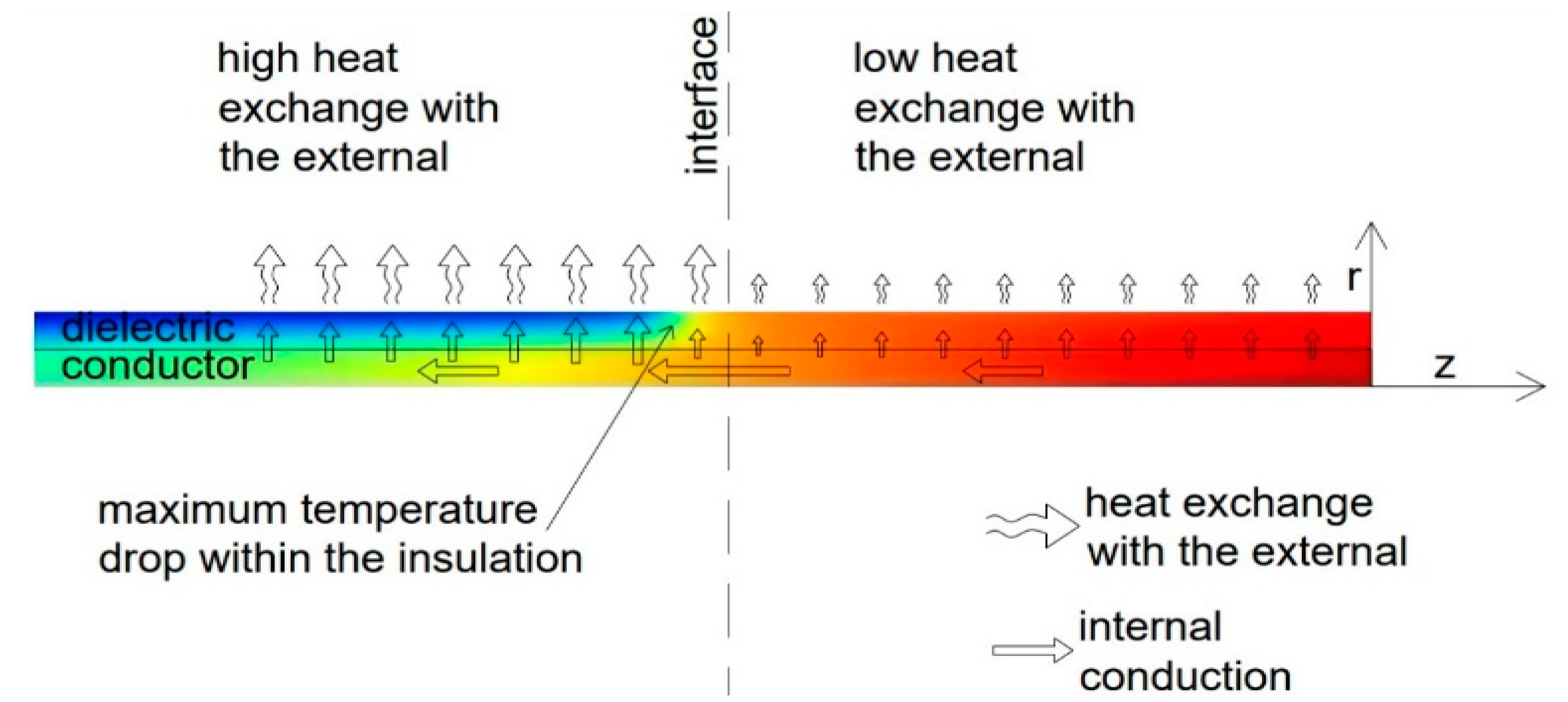
In this paper, attention is focused on the conditions that can lead to local and/or temporary peaks of thermal gradient in the dielectric layer of HVDC cables and the possibility to reach high levels of electric field near its external surface is verified. A discontinuity along the cable axis of the external heat exchange parameters can lead to the achievement of a local peak of temperature drop. In certain conditions, the axial thermal conduction can prevail on the radial one due to the high thermal conductivity of metals in comparison to that of polymeric materials. The area near a joint, the crossing by the cable of an interface between two different means or local external heat or cold sources are potentially cases in which axial heat transfer can play an important role in defining the highest electric field within the insulation of a cable. In Figure 1, the effect on the temperature drop of a hot spot is illustrated. Nevertheless, the large difference in the heat capacities of conductor and dielectric can temporarily increase the temperature drop during load transients. This can be amplified near geometric variations such as near joints.
The standards IEC 60853-2 and IEC 60287 propose procedures for the calculation of the temperature inside cables and for the current rating based on a one dimensional approach that neglect the axial heat transfer [13,14]. This is because these standards are applicable to AC cables or DC cables under less than 5 kV of voltage. In AC cables, the main parameter to be controlled is the conductor temperature and this is certainly achieved in the 2D section where the worst external heat exchange occurs. In this case, the axial heat conduction cannot further increase the conductor temperature in a hot spot.
To date, no dedicated standard of the International Electrotechnical Commission (IEC) provides a guide for the thermal design of HVDC cables at rated voltages greater than 5 kV. This lack is covered by the Cigrè brochure 640 [15] that takes into account the need to limit the temperature drop over the dielectric layer in HVDC cables. This document pays attention to the role of the axial heat transfer in the establishment of local variations in the radial temperature distribution. Some researchers have simulated the behavior of axial discontinuities by the thermal point of view by means of finite element analysis (FEA) in three-dimensional geometries [16,17,18]. However, this method requires high calculation powers.
To date, no standards have been dedicated to the calculation of the temperature profile and the current rating for HVDC cables. In the DC case, since the thermal gradient plays an important role in limiting the rated current, a 2D approach for modeling a laying section is not suitable to describe cautiously the operative conditions and a 3D modeling is necessary to take into account axial heat transfer phenomena.
The widespread ways to measure the radial pattern of space in cables are the pulsed electro acoustic (PEA) method and the thermal step method (TSM) [19,20,21,22,23,24]. In particular, the former is based on the detection of an acoustic impulse generated by the interaction between charges and a pulsed electric field externally generated. Due to the attenuation of acoustic signals when they pass through a solid material, the larger is the cable size, the lower is the measurable charge density. TSM is based on the measurements of a current of the order of pA proportional to the amount of space charge density. Due to the low levels of currents that are to be measured, this method is not suitable for measuring small space charge densities. Since the phenomena described above are more likely to occur in large HVDC cables, at the state of the art, experimental methods are not suitable for understanding the impact of axial discontinuities on the distribution of the electric field.
The establishment of a temperature gradient in the dielectric of HVDC cables plays an important role during programmed or accidental voltage transients [25].
In this paper, a 2D model in the radial and axial coordinates as well as in time domain is used to simultaneously calculate the distributions of temperature, space charge, and electric field.
Unlike the bipolar charge transport models used recently by other researchers, a conductivity model has been used in this research to evaluate the charge distribution in the dielectric [26]. Even if more approximate, the conductive model provides sufficiently reliable information for the evaluation of the electric field profile during a voltage transient [27].
In the second paragraph, the model implemented in Matlab® is described, whilst in the third, a case study is presented. Finally, the results are discussed in the fourth paragraph and further development ideas for future research are offered in the conclusions.
2. Mathematical Model
As mentioned above, a time domain 2D mathematical model has been developed to study the distribution of the electric field within the insulation of an HVDC cable close to a discontinuity along the axis of the heat exchange parameters with the external. The equations of the thermal and the electrical models are expressed in cylindrical geometry assuming axial symmetry. In this work, the angular heat conduction inside the cable is neglected in order to reduce the computational effort. The geometry of a typical HVDC cable is discretized into radial and axial nodes in order to model a multilayer stratigraphy such as the one shown in Figure 2. All the materials of the cable are modeled as continuous and homogeneous, therefore equivalent parameters are used for the stranded conductor and the wire screen in order to take into account their filling factor.
For each layer, thermal and electrical properties are assigned based on the materials as well as the tables of the standards IEC 60287 and IEC 60853-2.
The geometry is discretized in NR radial nodes and NZ axial nodes. For each of these, thermal conductivity, mass density, and specific heat characterize the material in the thermal model as well as permittivity and electrical conductivity at 20 °C are used in the electric model. All the parameters used in the thermal model are assumed constant and homogeneous for each material, whilst simplified equations are used for the calculation of electrical conductivity on dependence of temperature and electric field.
For metals, a linear relation between electrical conductivity and temperature is used considering the coefficient proposed by the standards above. In polymers, the electrical conductivity can be expressed as an exponential function of temperature and electric field. The model described in this article uses the following equation for the electrical conductivity of the dielectric:
where σ0 is the electrical conductivity at the temperature T0 and in absence of an external electric field, σ(T,E) is its value at the temperature T and under the electric field E expressed in V/m, a and b are the positive coefficient respectively for the temperature and the electric field. The reference temperature T0 is equal to 20 °C. The coefficient b is also variable with the temperature and it can be evaluated by means of the following:
where c, d, and e are parameters depending on the material. The Equation (2) and its coefficients are obtained by fitting the values reported in the reference [28]. The coefficient a is weakly variable with the electric stress but it can be considered as constant within the electric field ranges obtained in this work.
The distortion of the radial electric field profile in a loaded cable in comparison to the Laplacian field is mainly due to the temperature gradient. Indeed, the coefficient a is about 2–3 times higher than b in most of the commercial dielectric materials.
Due to the strong prevalence of the radial component of the electric field over the others, the variable E is here referred to the radial component of the electric field vector. In addition, due to its direct proportionality to the electrical field, the current density J is analogously referred to the radial component of the current density vector.
The volumetric heat source inside the conductor is calculated from the axial current density as function of time and the electric resistivity depending on the temperature. At the axial boundaries, an adiabatic condition is imposed whilst a convective heat transfer is considered at the radial external limit. This heat exchange mode is defined by an external temperature and a convective coefficient for each axial division of the geometry. The temperature distribution vs. time is calculated by means of the thermal conduction law in an axial-symmetric cylindrical coordinate system:
where r, z, and t are respectively the radial, the axial, and the time coordinates, k(r) is the thermal conductivity, q‴(r,z,t) is the thermal power density, rho(r) is the mass density, and C(r) is the specific heat. Equation (3) has been discretized in a linear system of NR*NZ equations through the finite differences method and iteratively solved for each time step.
Whilst the thermal model is applied to the entire cable segment, the domain of the electric model includes only the layers between the inner and the outer semicon and assumes that voltage is applied between these two layers. The electrical conductivity of the semicon layers is much greater than that of the dielectric, therefore the charge is accumulated at the interfaces in much faster times than those necessary for accumulation of the space charge within the insulation. This can lead to numerical instabilities during the transients, therefore the approach followed in this work is different for the dielectric and the semicon layers. It has been assumed that the space charge accumulated within the semicon layers reaches immediately a stationary value, therefore a stationary model has been applied to this portion of domain. This is complementary to the transient model applied to the dielectric layer.
By defining ND, the number of radial nodes that divide the insulation thickness, the electric model provides a set of linear systems each composed by ND*NZ equations in ND*NZ unknown values of radial components of the electric field E and current density J as well as space charge density . The electric field is calculated through the Gauss’s law expressed in cylindrical coordinates and assuming axial symmetry and neglecting variations along the axis:
where εr(r) is the relative permittivity of the material, ε0 is the vacuum dielectric constant and is the space charge density. Since at least two values of E are required to obtain a single value of , the differential Equation (4) can be discretized in a linear system of (ND − 1)*NZ equations in ND*NZ unknowns, where ND is the number of radial nodes that discretize the dielectric thickness.
As an initial condition, the space charge is considered equal to zero in the whole the domain. Consequently, the first radial distribution of the electrical field is a Laplacian pattern.
Once known, the temperature and the electric field in each node, the conductivity distribution can be calculated from Equations (1) and (2) in order to obtain the following:
The radial component of the current density through the dielectric can be therefore calculated from the Ohm’s law that can be simply applied to each node:
As it can be noted from (6), the current field depends on the electrical conductivity distribution and therefore on the thermal and electrical field. For most commercially used dielectric materials, the electrical conductivity is more dependent on the temperature than on the electric field.
By considering the assumption above, the current continuity equation expressed in cylindrical coordinates can be written as follows:
As it can be noted from the Equation (7), two values of J are needed for each discretized equation in , therefore, the linear system is closed, imposing a radial current density equal to zero in the dummy nodes outside the domain of the dielectric layer. This linear system of equations provides the distribution of the space charge inside the dielectric that can be introduced in the system obtained from the (4) at the subsequent time step.
As introduced above, a different approach has been followed to calculate the charge accumulated within the semicon layers. Since the time constants of this phenomena are proportional to the product between the electrical conductivity and permittivity, the charges accumulate in the semicon, near the interfaces with the dielectric, in a practically infinitesimal time compared to that required for accumulation inside the bulk of the dielectric. For this reason, a semi-stationary model has been developed to extend the linear systems of the equation deriving from the (4)–(7) to a domain containing the semicon layers. By setting the time variation of space charge equal to zero and introducing the (6) in the (7), the following equation is obtained:
The linear equations obtained from the Equation (8) can be added to those extrapolated from the (4) to forming a system of (NDL − 1) × NZ equations in NDL × NZ unknowns where NDL is the number of the radial nodes in which the layers between the external surface of the conductor and the inner surface of the shield are divided. In order to complete the linear system for the calculation of the electric field, the equation relating the electric field to the potential has to be used:
where rin and rout are respectively the inner and the outer radius of the dielectric layer and U(t) is the applied voltage. Equation (9) is discretized for each axial division and provides NZ equations to the linear system for the calculation of the electric field distribution.
Finally, the space charge distribution in the semicon layers is calculated from the (4) after obtaining the electric field distribution. In Figure 3, the calculation model is schematized.
In spite of a calculation through a commercial software using FEA, the procedure described in this article minimizes the computational effort. In order to take into account the axial heat transfer that plays an important role in proximity of axial discontinuities, a two dimensional approach is necessary for the thermal modeling. On the other hand, due to a negligible axial electric field and thermal gradient compared to their radial components, a one-dimensional approach is sufficient to model the charge and electric field distribution.
3. Boundary, Initial Conditions and Model Assumption of the Simulated Case Study
With the aim of evaluating the effect of an axial thermal flux in a HVDC cable, several simulations have been carried out varying the external temperature drop and the convective heat flux coefficient at the interface. A typical large size HVDC cable is reproduced in order to study the phenomenon under investigation. The sample cable has the geometrical and thermal characteristics shown in Table 1 [29,30]. The specific heats in Table 1, are obtained from the thermal capacities indicated in the IEC 60853-2 and the mass density of each material. This is with the aim of evaluating the linear weight of the sample cable. In Table 2, the electrical properties of the layers are shown. The values in Table 2 are referred to a temperature of 20 °C and an electric field of 5 kV/mm. With reference to Equation (1), the temperature coefficient a has been calculated by means of a linear interpolation between its values of 0.104 °C-1 and 0.114 °C-1 respectively under the electric fields of 20 and 30 kV/mm.
The values of b have been calculated in accordance to Equation (2) and adopting the following coefficients: c = −4.13 × 10⁻¹¹ m/(V × K2), d = 2.83 × 10⁻⁹ m/(V × K), e = 1.25 × 10⁻⁸ m/V. These parameters are compatible with those of a thermoplastic dielectric material. The study has been carried out on a section of 6 m of HVDC cables exchanging heat with the external by means of convection. Since the thermal model is two-dimensional, the different external temperature and convective heat exchange coefficient can be set along the axial coordinate of the cable. Different levels of variation are simulated in order to evaluate the dependence between the maximum electric field and the axial variation of the outer thermal conditions.
The radial electric field distribution over the radius and the axis of the modeled cable section has been calculated in steady state conditions and during a PR event.
The transient has a duration of 24 h with the electrical boundary conditions shown in Table 3. This scenario is compatible with a slow PR event [31]. In order to investigate the behavior of the phenomenon with different thermal boundary conditions, five different scenarios have been simulated. In Table 4, the external temperature and the convective heat transfer coefficients are shown for the simulated scenarios. These parameters have been assumed to vary linearly in an axial length of 0.3 m in proximity of the center of the 6 m long modeled cable portion.
The values of the external temperature and convective coefficients are compatible with an external cooling in water and air. In particular, the portion of the cable with an axial coordinate of less than 2.7 m is immersed in water, whilst the remaining part exchanges heat with the air. As can be seen from Table 4, only the heat exchange parameters in the air-cooled region are varied in the different scenarios. This choice has been made with the aim of comparing the maximum values of the electric field reached in proximity of the water–air interface with reference values relating to the portion of cable immersed in water and sufficiently distant from the liquid surface.
4. Results and Discussion
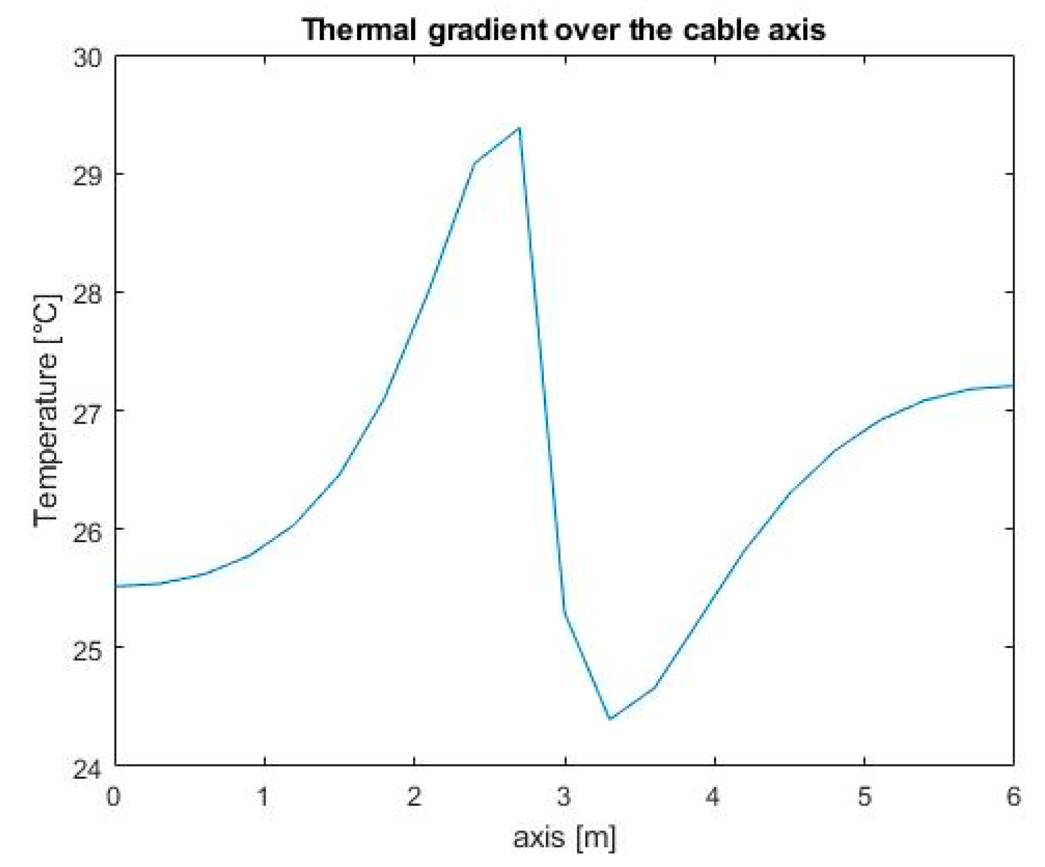
In this section, the results of the simulations of the above described scenarios are shown. In Figure 4, an example of the axial distribution of temperature drop over the dielectric layer is shown. The illustrated graph refers to Scenario E, in which the maximum local peak of the thermal drop is reached.
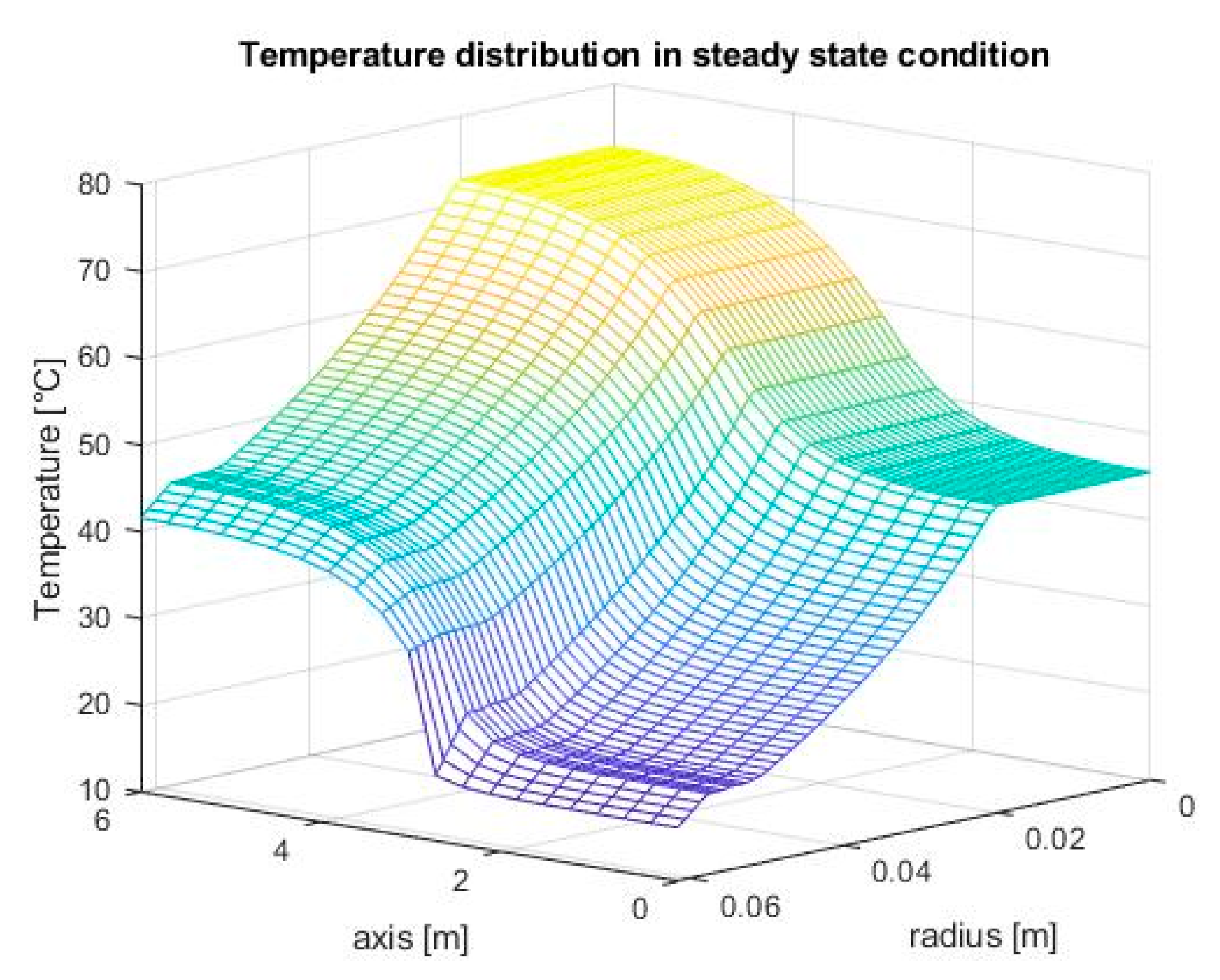
With the aim of illustrating the role of the interface on the steady state temperature distribution over the radius and the axis of the modeled cable portion, a 3D graph is illustrated in Figure 5. As it can be observed, the temperature drop reaches its peak just above the liquid level in accordance with the initial hypothesis illustrated in Figure 1. The hottest part of the cable exchanging heat with still air heats up the coldest part by means of conduction through the cable core. Therefore, the conductor of the cable just below the liquid level has almost the same temperature of the portion cooled in air whilst the external surface in the same axial position is cooled with a high convection coefficient by the water. Consequently, a thermal gradient peak is expected at the interface between the two different means by which the cable exchanges heat. In stationary conditions for Scenario E, it has been found that the thermal drop at the interface is 1.15 times greater than the portion cooled in water and 2.7 m below the liquid level.
In Figure 5, it can be seen that the temperature at the external boundary of the cable in the portion immersed in air is more than 15 °C higher than the environmental temperature set for Scenario E. This shows that the axial thermal transmission through the core depends more on the variation of the convective coefficient at the interface than on the variation of temperature.
As specified above, the presence of a radial thermal gradient causes the onset of a high conductivity gradient due to the exponential law of dependence of the electric conductivity on the temperature and this leads to the accumulation of space charge within the dielectric.
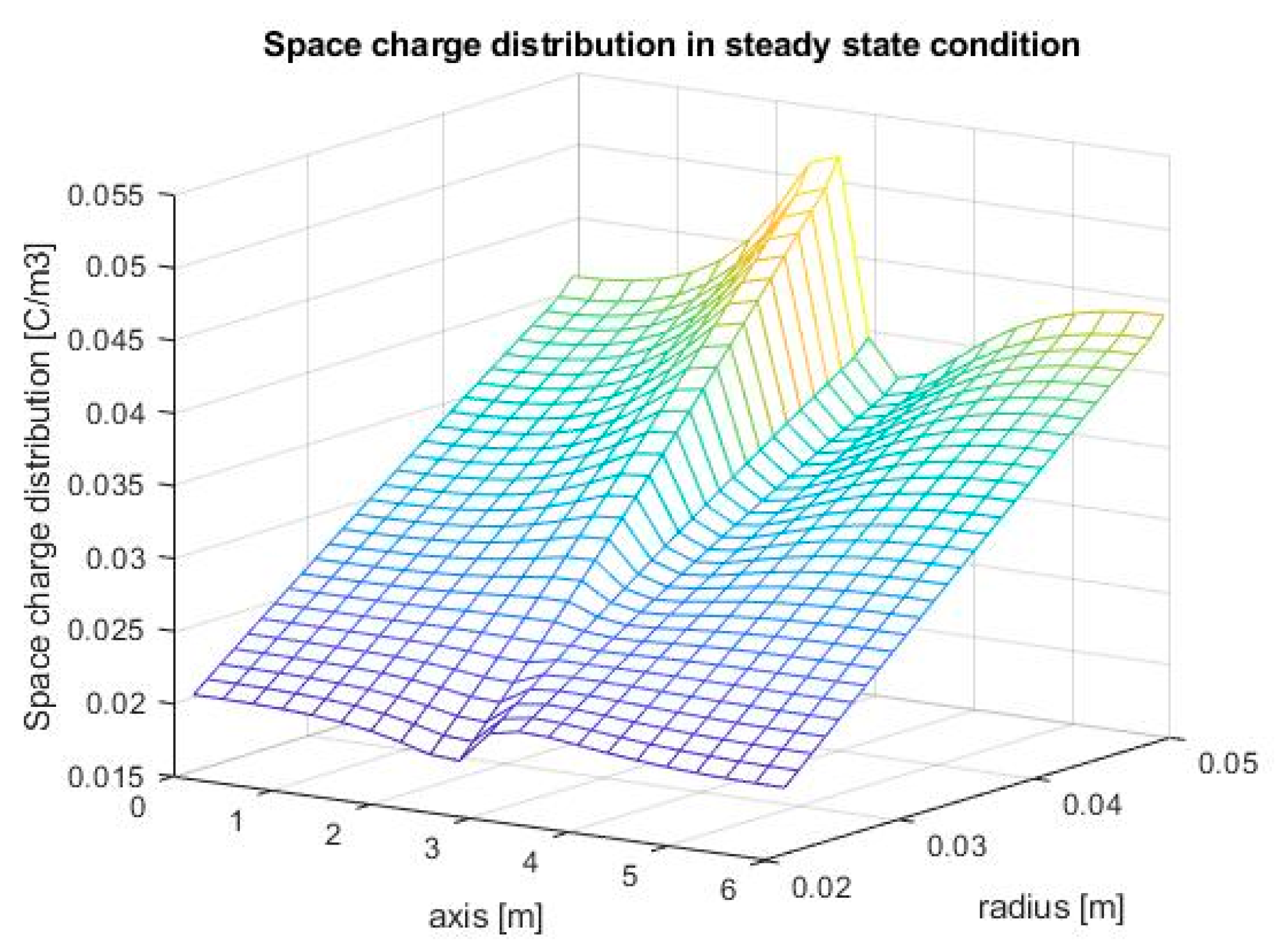
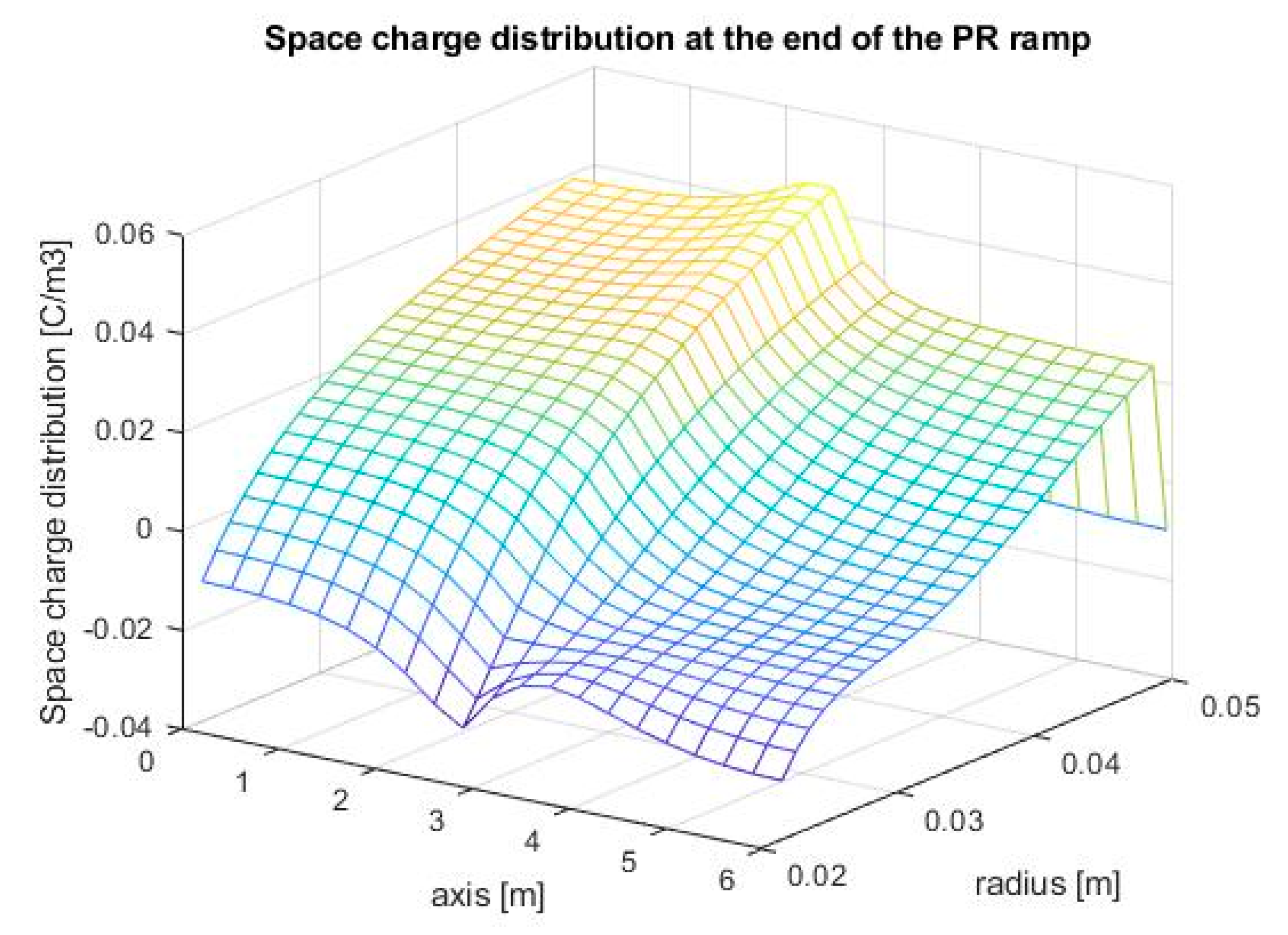
In Figure 6, the steady state space charge distribution within the insulation layer is illustrated by means of a 3D graph. As can be noted, peak value is reached just below the liquid level in proximity of the outer boundary, following the same trend of the axial distribution of the thermal drop shown in Figure 4. In the stationary conditions for Scenario E, the maximum space charge density at the liquid level has been found to be 1.27 times greater than that in the portion cooled in water and 2.7 m below the interface. As it can be expected, the accumulation of space charge leads to inversion of the radial electric field profile with the maximum absolute values reached in proximity of the external surface of the dielectric layer.
In Figure 7, the steady state radial electric field distribution over the radius and the axis of the cable is shown. In the stationary conditions for Scenario E, the maximum electric field at the liquid level is 1.11 times greater than the portion cooled in water and 2.7 m below the liquid level. It can be stated that, in stationary conditions, the local increase in the electric field caused by the effect of an interface between two means in which an HVDC cable is immersed depends on the local increase in the thermal gradient. Nevertheless, the maximum value of the steady state electric field depends on the local temperature gradient close to the external surface of the dielectric layer.
The same temperature drop over the entire thickness can be achieved with different radial thermal profiles, therefore, contrary to what may appear in a first approximation, there is not a proportional dependence between the increase in thermal drop and the increase in local electric field at the interface. It is more correct to state that the local peak of electric field depends both on the temperature difference between the two means at the interface and of the ratio between the convective coefficients.
In Table 5, the main results of the simulated scenarios in steady state conditions are shown in terms of increases in thermal drop, space charge and radial electric field respect to the reference values reached 2.7 m below the liquid level. As it can be noted from the Table, the maximum steady state value of the electric field is achieved in Scenario E and it is equal to 33.7 kV/mm.
Once the steady state conditions have been reached from the thermal and electrical points of view, a PR event has been simulated as specified in Table 3. In all simulated scenarios, the maximum electric field was reached at the end of the PR ramp, in proximity of the internal boundary of the dielectric, in the area most distant from the interface and immersed in water.
In order to illustrate the temporal trend of the maximum absolute value of the electric field during the simulated transient, the graphs shown in Figure 8 and Figure 9 have been drawn. These graphs refer to Scenario D, during which the maximum peak of the electric field has been achieved. It should be noted that Scenario D is characterized by the lowest increases in temperature drop and consequently in electric field during the stationary phase. However, the maximum values of the electric field reached at the end of the PR ramp in all the simulated scenarios are all at most 1% lower than the peak found during Scenario D. This is because the thermal distribution 2.7 m below the liquid level is not strongly dependent on the heat exchange conditions of the portion immersed in air.
With reference to Figure 8 and Figure 9, it can be noted an initial reduction of the electric stress due to the inversion of the profile of the electric field after the application of the load and starting from a homogeneous temperature distribution. As described above, due to the establishment of a thermal gradient, the electric field tends to reduce its value in proximity of the internal boundary whilst reaching its maximum at the external. The time necessary to achieve a stationary electric field distribution depends on the time constants of the thermal and electrical phenomena. The former is strictly related to the cable weight, whilst the latter can be expressed as the product between the permittivity and the conductivity of the dielectric material. Since the electrical conductivity of polymers is dependent on the temperature with exponential law, the electrical time constant varies up to 3 orders of magnitude within the operating thermal range in which the cable works. This can play an important role during relative fast voltage transients such as PRs and TOVs.
After reaching a minimum value, the maximum electric field module starts to rise again, reaching an asymptotic value in approximately 15 h. Once the steady state is achieved, the electric field suddenly collapses due to grounding in 1 s of the conductor.
After a relaxing phase of 180 s, the maximum electric field suddenly reaches its peak at the end of the ramp of the PR. This peak is achieved at the internal boundary of the dielectric layer in the coldest region of the cable. Afterwards, its value begins to decrease, falling below the asymptotic value previously reached in about 2 min.
Approximately 7 min after the inversion, the electric field at the outer surface of the insulation in the air-cooled part exceeds that at the inner boundary in the area immersed in water. This new maximum is in turn overcome, after about 90 min, by the electric field at the external surface of the dielectric close the interface. The latter finally reaches an asymptotic value identical to that reached before the PR.
The maximum values of the electric field found at the end of the PR depends not only on the temperature drop over the insulation but also on its average value within the dielectric. Indeed, at higher temperature, the greater charge mobility reduces the time necessary for the relaxation. In example, due to their lower operating temperature, mass impregnated non-draining (MIND) cables could be stressed by higher electric field peaks during a PR [32].
In Figure 10, a comparison is made between profiles of the radial electric field at different times during the transient of the Scenario D in the coldest area of the modeled cable portion. As it can be observed, the maximum value of the electric field achieved in proximity of the external surface of the dielectric before the PR is higher than that reachable in no load conditions at the internal boundary. Once the PR ramp is finished, the electric field achieves its maximum value of 39.27 kV/mm, 19% higher than the maximum steady state value reached on the external surface and near the interface. In this instant, whilst a negative peak is reached at the internal boundary, a residual positive electric field can be observed in proximity of the outer surface. This is due to the lower mobility of the charges at low temperatures. In light of the above, it is evident that a sudden variation along the axis of the thermal conditions outside a cable causes the achievement of local peaks of the electric field in stationary conditions. On the contrary, this scenario has a negligible influence during an event of PR. In order to better explain this behavior, the electric field distribution and the space charge at different times of the Scenario E have been analyzed.
In Figure 11, the space charge distribution calculated for Scenario E at the end of the PR ramp is shown. As it can be observed, the minimum absolute value of the space charge density is reached in the area cooled in water and farthest from the surface. Here, the effect of the application of a negative voltage is combined with a lower mobility of the charges due to the lower temperature compared to the portion of the cable cooled in air. Therefore, in this area, during the PR ramp, the effect of the reduced mobility of the charges due to relatively lower temperatures appears to prevail over that related to the temperature gradient.
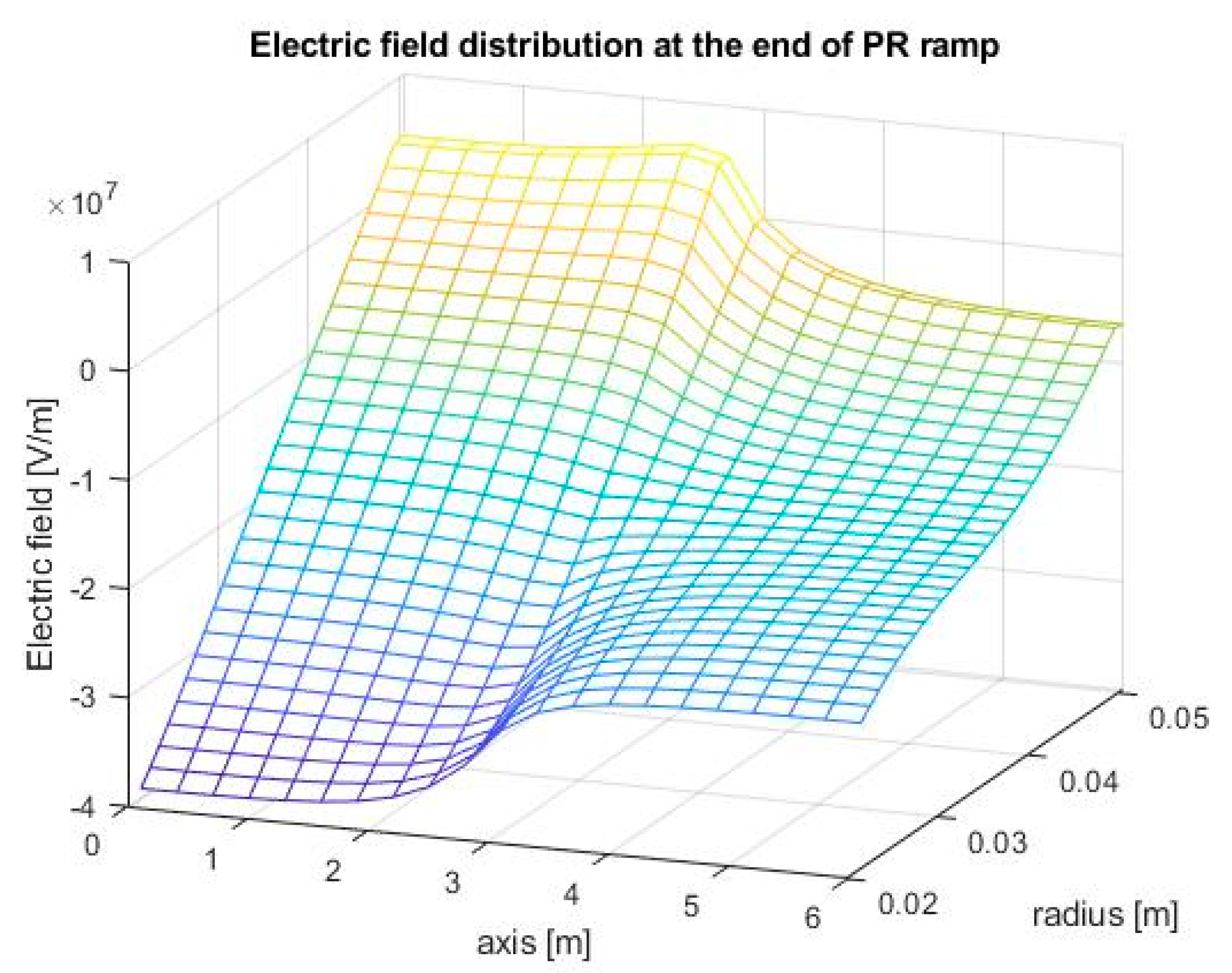
In Figure 12, the distribution of the electric field at the end of the PR ramp is shown. As it can be observed, the electric field gradient in the portion of cable immersed in water is higher than that cooled in air. In this colder area, the residual positive electric field in proximity of the external surface can be attributed to a higher electric time constant for the space charge re-distribution. During this phase, the maximum value of the electric field depends strongly on the absolute temperature of the dielectric and, consequently, also on the current flowing through the cable.
If on one hand the space charge increases with the thermal gradient and therefore with the load, on the other, the mobility of the charges is reduced with the lowering of the current. It is therefore possible that a load condition can be determined that maximizes the local electric field as a function of the external heat exchange conditions.
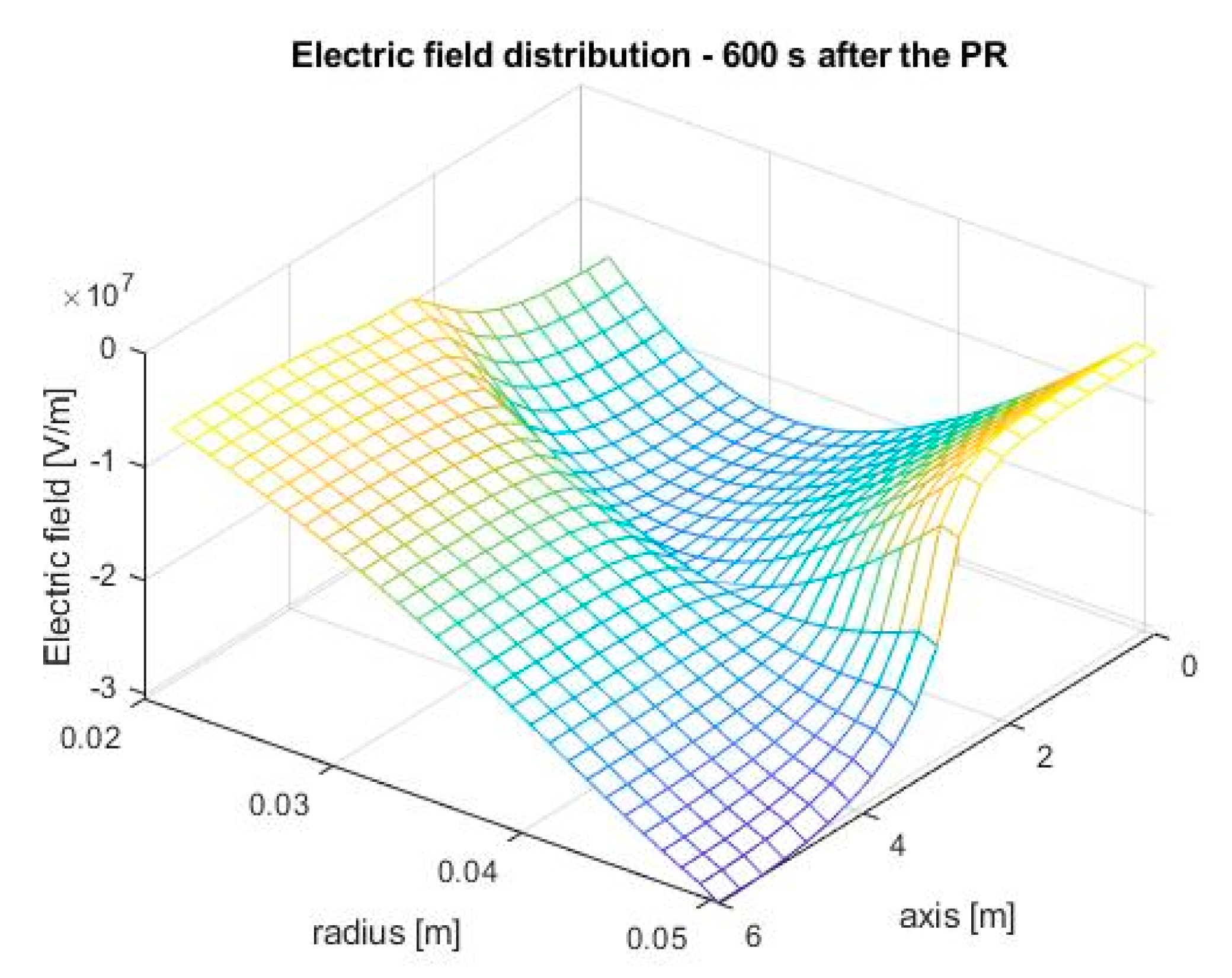
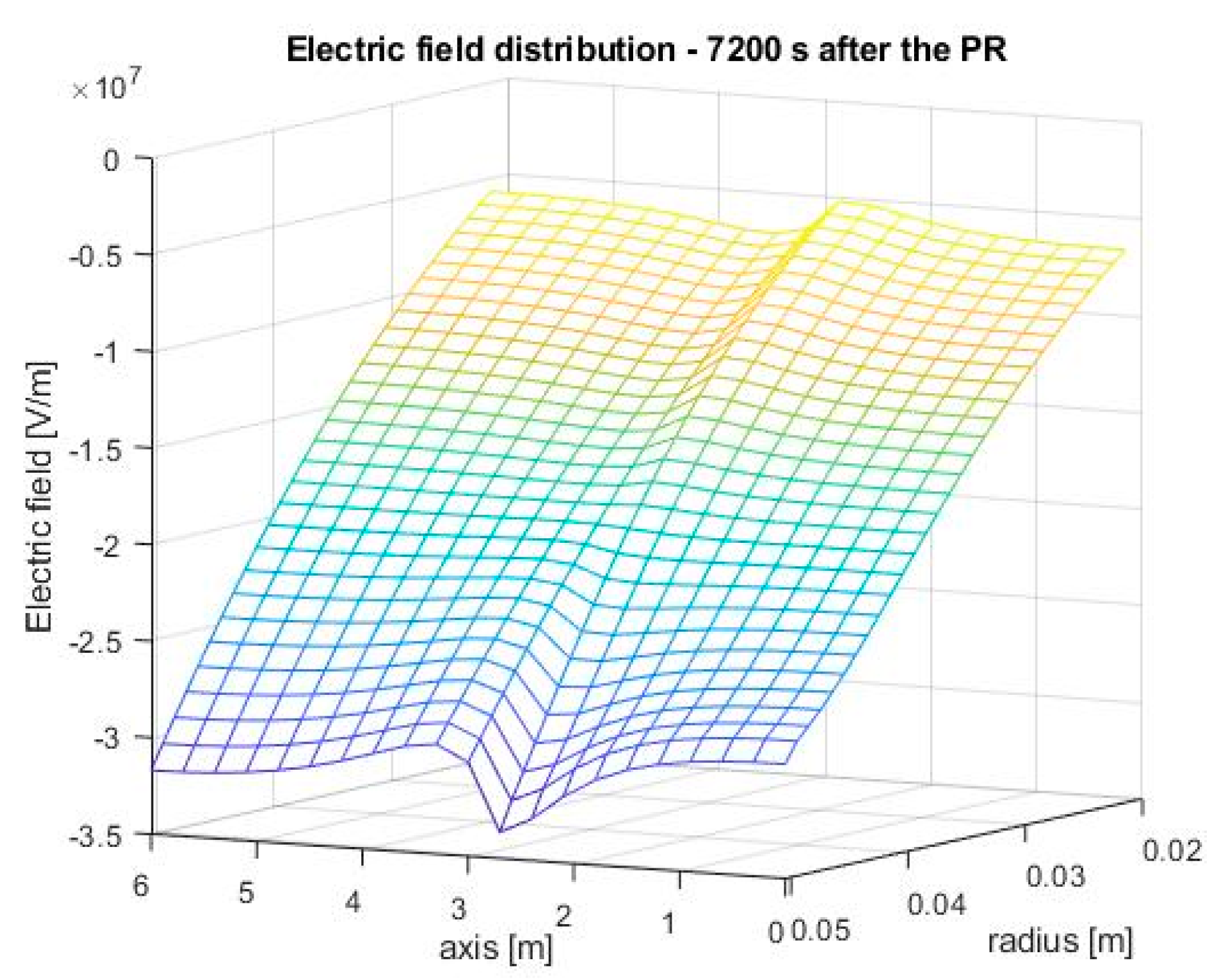
In Figure 13, the electric field distribution after 10 min from the PR is shown. At this step, the charge re-distribution in the colder area is still not complete, therefore, in this portion, the electric field reaches its maximum in proximity of the middle of the dielectric thickness. On the other hand, the electric field distribution in the portion immersed in air has already reached almost steady state conditions which, in a specular way, tend to those illustrated in Figure 7. As it can be observed in Figure 14, after approximately 2 h after the PR, a new equilibrium condition has been reached.
In light of the above, it can be stated that the time required to reach new stationary conditions after a voltage transient increases with the lowering of the temperature in the dielectric.
5. Conclusions
This paper describes the results of a study on the role of the axial heat transfer in HVDC cables on the space charge accumulation phenomena. Because of the accumulation of space charge, the electric field distribution departs from the Laplacian profile and it is conditioned from the thermal field.
In addition to the authors’ previous work, the evolution of the space charge and electric field distributions have been investigated under five different scenarios [33]. Moreover, an analysis of the electric field peaks reached during and after a PR event has been carried out.
With the aim of performing numerical simulation to carry out this study, a thermal and electric model has been developed in time domain. This model takes into account the accumulation of space charge caused by the dependence of the electrical conductivity of the dielectric on the temperature. It should be stressed that other issues contribute to the space charge phenomena in HVDC cables. As demonstrated in recent studies, these issues, simulated as conductivity discontinuities, play an important role in the increase of the space charge density within the dielectric [34]. Nevertheless, the effect of the temperature drop over the dielectric layer has a weight, between the other space charge phenomena, increasing with the sizes of the cable.
In the case study analyzed in this article, a segment of an HVDC cable 6 m long has been modeled by means of a cylindrical axial-symmetric two-dimensional geometry. It has been considered that the insulation of the cable consists of a thermoplastic material whose thermal and electrical characteristics are available in the literature.
A portion of a full size HVDC cables has been modeled considering a half in length cooled in water and the other in air. In this way, the effect of the axial variation in the external thermal conditions on the radial temperature gradient has been assessed. This causes the onset of a local peak in the temperature drop over the dielectric layer just below the liquid level. As was found in the previous work of the authors, the results of this research show that the presence of the interface between the two external means plays an important role in the determining of electric field distribution due to a greater amount in this area of space charge. The increase in electric field reached just below the liquid level seems to be almost proportional to the temperature drop growth at the interface. The thermal gradients obtained in this research are comparable to those occurring in operating large size cables. The effect of the sudden axial variation in the thermal conditions can result amplified during emergency loading or fast load transients.
The findings of this research show no appreciable dependence between the peak of electric field reached during a slow PR event and the effect of an interface between 2 means out of the cable. On the contrary, at the end of a PR ramp, the maximum value of the electric field is achieved in the coldest area of the modeled cable. This phenomenon can be explained by the lower mobility of the space charge where the dielectric temperature is lower. This effect seems to prevail on the lower thermal drop in the most cooled areas of the cable.
The findings of this work are referred to a specific case study but they are extendible to other scenarios in which the radial temperature distribution is conditioned by axial discontinuities by the thermal point of view. Therefore, this study can be extended to other cases in order to assess the actual electric field distribution in proximity of joints, hot and cold points along the line or the proximity to other heat sources.
The research offered in this article attempts to provide a contribution for a deeper understanding of the phenomenon of the accumulation of space in large HVDC cables and of its consequences in terms of achieving high levels of electric field. This and other works on this topic may provide elements to take into account in the thermal rating of HVDC cables.
Author Contributions
Conceptualization, G.R.; Data curation, G.R.; Formal analysis, P.R. and F.V.; Investigation, G.R. and A.I.; Methodology, G.R.; Resources, P.R.; Supervision, G.A.; Writing—original draft, G.R.; Writing—review & editing, P.R. All authors have read and agreed to the published version of the manuscript.
Funding
This research received no external funding.
Conflicts of Interest
The authors declare no conflict of interest.
Acronyms
| AC | Alternating Current |
| DC | Direct Current |
| FEA | Finite Element Analysis |
| HVDC | High Voltage Direct Current |
| IEC | International Electrotechnical Commission |
| MIND | Mass Impregnated Non-Draining |
| PEA | Pulsed Electro-Acoustic |
| PR | Polarity Reversal |
| TOV | Transient Over Voltage |
| TSM | Thermal Step Method |
Variables and Parameters
| a | temperature coefficient for the electrical conductivity |
| b | electric field coefficient for the electrical conductivity |
| c | first parameter for the evaluation of the coefficient b |
| C(r) | specific heat at the radial coordinate r |
| d | second parameter for the evaluation of the coefficient b |
| e | third parameter for the evaluation of the coefficient b |
| E(r,z,t) | radial component of the electric field at the coordinates r, z, t |
| J(r,z,t) | radial component of the current density at the coordinates r, z, t |
| k(r) | radial thermal conductivity at the radial coordinate r |
| ND | radial nodes in which the insulation thickness is discretized |
| NDL | radial nodes in which the layers between the external surface of the conductor and the inner surface of the shield are discretized |
| NR | Radial nodes in which the cable geometry is discretized |
| NZ | Axial nodes in which the cable geometry is discretized |
| q‴(r,z,t) | thermal power density at the coordinates r, z, t |
| r | radial coordinate |
| rho(r) | mass density at the radial coordinate r |
| rin | inner radius of the dielectric layer |
| rout | outer radius of the dielectric layer |
| t | time coordinate |
| T(r,z,t) | temperature at the coordinates r, z, t |
| T0 | reference temperature (20 °C) |
| U(t) | applied voltage at the time t |
| z | axial coordinate |
| ε0 | vacuum dielectric constant |
| εr(r) | relative permittivity at the radial coordinate r |
| σ(T,E) | electrical conductivity at the temperature T and the electric field E |
| σ0 | electrical conductivity at the temperature T0 and electric field equal to 0 |
| space charge density at the coordinates r, z, t |
References
- Imburgia, A.; Romano, P.; Sanseverino, E.R.; Viola, F.; Hozumi, N.; Morita, S. Space charge behavior of different insulating materials employed in AC and DC cable systems. In Proceedings of the 2017 International Symposium on Electrical Insulating Materials (ISEIM), Toyohashi, Japan, 11–15 September 2017; pp. 629–632. [Google Scholar] [CrossRef]
- Romano, P.; Imburgia, A.; Candela, R. Space Charge Measurement under DC and DC Periodic Waveform. In Proceedings of the 2018 IEEE Conference on Electrical Insulation and Dielectric Phenomena (CEIDP), Cancun, Mexico, 21–24 October 2018; pp. 293–296. [Google Scholar]
- Andrade, M.D.A.; Candela, R.; De Rai, L.; Imburgia, A.; Sanseverino, E.R.; Romano, P.; Troia, I.; Viola, F. Different Space Charge Behavior of Materials Used in AC and DC Systems. In Proceedings of the 2017 IEEE Conference on Electrical Insulation and Dielectric Phenomenon (CEIDP), Fort Worth, TX, USA, 22–25 October 2017; pp. 114–117. [Google Scholar]
- Imburgia, A.; Romano, P.; Viola, F.; Madonia, A.; Candela, R.; Troia, I. Space charges and partial discharges simultaneous measurements under DC stress. In Proceedings of the 2016 IEEE Conference on Electrical Insulation and Dielectric Phenomena (CEIDP), Toronto, ON, Canada, 16–19 October 2016; pp. 514–517. [Google Scholar]
- Romano, P.; Imburgia, A.; Ala, G. Partial Discharge Detection Using a Spherical Electromagnetic Sensor. Sensors 2019, 19, 1014. [Google Scholar] [CrossRef] [PubMed] [Green Version]
- Montanari, G.C. Bringing an insulation to failure: The role of space charge. IEEE Trans. Dielectr. Electr. Insul. 2011, 18, 339–364. [Google Scholar] [CrossRef]
- Fabiani, D.; Montanari, G.C.; Laurent, C.; Teyssedre, G.; Morshuis, P.; Bodega, R.; Dissado, L. HVDC Cable Design and Space Charge Accumulation. Part 3: Effect of Temperature Gradient [Feature article]. IEEE Electr. Insul. Mag. 2008, 24, 5–14. [Google Scholar] [CrossRef]
- Christoph, J.; Clemens, M. Electric Field Model at Interfaces in High Voltage Cable Systems. In Proceedings of the 2019 19th International Symposium on Electromagnetic Fields in Mechatronics, Nancy, France, 29–31 August 2019; pp. 1–3. [Google Scholar]
- Jiang, Y.; Liang, Z.; Su, S.; Zhang, X.; Li, L. Calculation of Electric Field in HVDC Cable. In Proceedings of the 2019 6th International Conference on Information Science and Control Engineering (ICISCE), Shanghai, China, 20–22 December 2019; pp. 1013–1016. [Google Scholar]
- Jorgens, C.; Clemens, M. Comparison of Two Electro-Quasistatic Field Formulations for the Computation of Electric Field and Space Charges in HVDC Cable Systems. In Proceedings of the 2019 22nd International Conference on the Computation of Electromagnetic Fields (COMPUMAG), Paris, France, 15–19 July 2019; pp. 1–4. [Google Scholar]
- Jörgens, C.; Clemens, M. Simulation of the Electric Field in High Voltage Direct Current Cables and the Influence on the Environment. In Proceedings of the Tenth International Conference on Computational Electromagnetics (CEM 2019), Edinburgh, UK, 19–20 June 2019; pp. 1–5. [Google Scholar]
- Setiawan, A.; Seri, P.; Cavallini, A.; Suwarno, S.; Naderiallaf, H. The Influence of Nanocomposite Filler on the Lifetime Performance of Polypropylene under Voltage Polarity Reversal. In Proceedings of the 2019 2nd International Conference on High Voltage Engineering and Power Systems (ICHVEPS), Denpasar, Indonesia, 1–10 October 2019; pp. 047–051. [Google Scholar]
- International Electro Technical Commission. IEC 60853-2. Calculation of the Cyclic and Emergency Current Ratings of Cables. Part 2: Cyclic Rating Factor of Cables Greater than 18/30 (36) kV and Emergency Ratings for Cables of All Voltages; IEC: Geneva, Switzerland, 1989. [Google Scholar]
- International Electro Technical Commission. IEC 60287-1. Calculation of Current Rating Part 1: (100% Load Factor) and Calculation of Losses; IEC: Geneva, Switzerland, 2001. [Google Scholar]
- CIGRE TB 640. A Guide for Rating Calculations of Insulated Cables; CIGRE: Paris, France, 2015.
- Pilgrim, J.A.; Swaffleld, D.; Lewin, P.; Payne, D. An Investigation of Thermal Ratings for High Voltage Cable Joints through the use of 2D and 3D Finite Element Analysis. In Proceedings of the Conference Record of the 2008 IEEE International Symposium on Electrical Insulation, Vancouver, BC, Canada, 9–12 June 2008; pp. 543–546. [Google Scholar]
- Pilgrim, J.A.; Swaffield, D.; Lewin, P.L.; Larsen, S.; Payne, D. Assessment of the Impact of Joint Bays on the Ampacity of High-Voltage Cable Circuits. IEEE Trans. Power Deliv. 2009, 24, 1029–1036. [Google Scholar] [CrossRef]
- Huang, Z.Y.; Pilgrim, J.A.; Lewin, P.L.; Swingler, S.G.; Tzemis, G. Thermal-Electric Rating Method for Mass-Impregnated Paper-Insulated HVDC Cable Circuits. IEEE Trans. Power Deliv. 2014, 30, 437–444. [Google Scholar] [CrossRef]
- Ala, G.; Caruso, M.; Cecconi, V.; Ganci, S.; Imburgia, A.; Miceli, R.; Romano, P.; Viola, F. Review of acoustic methods for space charge measurement. In Proceedings of the 2015 AEIT International Annual Conference (AEIT), Naples, Italy, 14–16 October 2015; pp. 1–6. [Google Scholar]
- Imburgia, A.; Miceli, R.; Sanseverino, E.R.; Romano, P.; Viola, F. Review of space charge measurement systems: Acoustic, thermal and optical methods. IEEE Trans. Dielectr. Electr. Insul. 2016, 23, 3126–3142. [Google Scholar] [CrossRef]
- Imburgia, A.; Romano, P.; Caruso, M.; Viola, F.; Miceli, R.; Sanseverino, E.R.; Madonia, A.; Schettino, G. Contributed Review: Review of thermal methods for space charge measurement. Rev. Sci. Instrum. 2016, 87, 111501. [Google Scholar] [CrossRef] [PubMed] [Green Version]
- Imburgia, A.; Romano, P.; Sanseverino, E.R.; De Rai, L.; Bononi, S.F.; Troia, I. Pulsed Electro-Acoustic Method for specimens and cables employed in HVDC systems: Some feasibility considerations. In Proceedings of the 2018 AEIT International Annual Conference, Bari, Italy, 3–5 October 2018; pp. 1–6. [Google Scholar]
- Rizzo, G.; Romano, P.; Imburgia, A.; Ala, G. Review of the PEA Method for Space Charge Measurements on HVDC Cables and Mini-Cables. Energies 2019, 12, 3512. [Google Scholar] [CrossRef] [Green Version]
- Imburgia, A.; Romano, P.; Chen, G.; Rizzo, G.; Sanseverino, E.R.; Viola, F.; Ala, G. The Industrial Applicability of PEA Space Charge Measurements, for Performance Optimization of HVDC Power Cables. Energies 2019, 12, 4186. [Google Scholar] [CrossRef] [Green Version]
- Adi, N.; Vu, T.T.N.; Teyssedre, G.; Baudoin, F.; Sinisuka, N. DC Model Cable under Polarity Inversion and Thermal Gradient: Build-Up of Design-Related Space Charge. Technologies 2017, 5, 46. [Google Scholar] [CrossRef] [Green Version]
- Zhan, Y.; Chen, G.; Hao, M. Space charge modelling in HVDC extruded cable insulation. IEEE Trans. Dielectr. Electr. Insul. 2019, 26, 43–50. [Google Scholar] [CrossRef] [Green Version]
- Zhan, Y.; Chen, G.; Hao, M.; Pu, L.; Zhao, X.; Sun, H.; Wang, S.; Guo, A.; Liu, J. Comparison of two models on simulating electric field in HVDC cable insulation. IEEE Trans. Dielectr. Electr. Insul. 2019, 26, 1107–1115. [Google Scholar] [CrossRef]
- Mazzanti, G.; Marzinotto, M. Extruded Cables for High-Voltage Direct-Current Transmission—Advances in Research and Development; John Wiley & Sons, Inc.: Hoboken, NJ, USA, 2013. [Google Scholar]
- Lee, K.-Y.; Nam, J.-C.; Park, D.-H.; Park, D.-H. Electrical and thermal properties of semiconductive shield for 154 kV power cable. In Proceedings of the 2005 International Symposium on Electrical Insulating Materials, (ISEIM 2005), Kitakyushu, Japan, 5–9 June 2005; Volume 3, p. 616. [Google Scholar]
- Heinrich, R. Broadband measurement of the conductivity and the permittivity of semiconducting materials in high voltage XLPE cables. In Proceedings of the Eighth International Conference on Dielectric Materials, Measurements and Applications, Edinburgh, UK, 17–21 September 2000; pp. 212–217. [Google Scholar]
- Marzinotto, M.; Battaglia, A.; Mazzanti, G. Space charges and life models for lifetime inference of HVDC cables under voltage polarity reversal. In Proceedings of the 2019 AEIT HVDC International Conference (AEIT HVDC), Florence, Italy, 9–10 May 2019; pp. 1–5. [Google Scholar]
- Battaglia, A.; Marzinotto, M.; Mazzanti, G. A Deeper Insight in Predicting the Effect of Voltage Polarity Reversal on HVDC Cables. In Proceedings of the 2019 IEEE Conference on Electrical Insulation and Dielectric Phenomena (CEIDP), Richland, WA, USA, 20–23 October 2019; pp. 442–445. [Google Scholar]
- Rizzo, G.; Romano, P.; Imburgia, A.; Viola, F.; Schettino, G.; Giglia, G.; Ala, G. Space charge accumulation in undersea HVDC cables as function of heat exchange conditions at the boundaries—water-air interface. In Proceedings of the 2020 IEEE 20th Mediterranean Electrotechnical Conference (MELECON), Palermo, Italy, 16–18 June 2020; pp. 447–452. [Google Scholar]
- Ren, H.; Zhong, L.; Yang, X.; Li, W.; Gao, J.; Yu, Q.; Chen, X.; Li, Z. Electric field distribution based on radial nonuniform conductivity in HVDC XLPE cable insulation. IEEE Trans. Dielectr. Electr. Insul. 2020, 27, 121–127. [Google Scholar] [CrossRef]
Figure 1.
Schematic of prevalent axial conduction close to an interface between two external means.

Figure 2.
Typical high voltage direct current (HVDC) large size cable.

Figure 3.
Scheme of the calculation model.

Figure 4.
Axial distribution of thermal drop—Scenario E.

Figure 5.
Temperature vs. radius and axis in steady state conditions—Scenario E.

Figure 6.
Space charge vs. radius and axis in steady state conditions—Scenario E.

Figure 7.
Electric field vs. radius and axis in steady state conditions—Scenario E.

Figure 8.
Maximum absolute value of electric field in the modeled cable portion—Scenario D.

Figure 9.
Maximum absolute value of electric field in the modeled cable portion—Scenario D, detail.

Figure 10.
Radial electric field distributions—Scenario D.

Figure 11.
Space charge distribution at the end of the Polarity Reversal (PR) ramp—Scenario E.

Figure 12.
Electric field distribution at the end of the PR ramp—Scenario E.

Figure 13.
Electric field distribution 600 s after the end of the PR ramp—Scenario E.

Figure 14.
Electric field distribution 7200 s after the end of the PR ramp—Scenario E.


Table 1.
Geometrical and physical properties of the cable taken as the case study.
| Layer | Description | External Radius [mm] | Mass Density [kg/m3] | Specific Heat [J/kgK] | Thermal Conductivity [W/mK] |
|---|---|---|---|---|---|
| 1 | Conductor 1 | 20 | 8960 | 385 | 390 |
| 2 | Inner semicon | 21 | 1180 | 1900 | 0.6 |
| 3 | dielectric | 51 | 1400 | 1714 | 0.2857 |
| 4 | outer semicon | 52 | 1180 | 1900 | 0.6 |
| 5 | swelling tape | 53 | 930 | 1900 | 0.6 |
| 6 | metallic screen 1 | 55 | 8960 | 385 | 390 |
| 7 | swelling tape | 56 | 930 | 1900 | 0.6 |
| 8 | aluminum laminate | 58 | 2700 | 896 | 290 |
| 9 | PVC outer covering | 62 | 1400 | 1214 | 0.167 |
1 Filling factors are taken into account by means of effective lumped parameters.
Table 2.
Electrical properties of the cable taken as the case study.
| Layer | Description | Permittivity | Reference Resistivity (@20 °C) [Ohm × m] |
|---|---|---|---|
| 2 | Inner semicon | 5000 | 2.18 |
| 3 | dielectric | 2.5 | 1.4 × 10¹⁴ |
| 4 | outer semicon | 5000 | 2.18 |
| 5 | swelling tape | 5000 | 2.18 |
Table 3.
Electrical boundary conditions during the simulated transient.
| Time [s] | Conductor Voltage [kV] | Screen Voltage [kV] | Current [A] |
|---|---|---|---|
| 0–60480.0 | 510 | 0 | 1700 |
| 60480.0–60481.0 | From 510 to 0 | 0 | 0 |
| 60481.0–60661.0 | 0 | 0 | 0 |
| 60661.0–60662.0 | From 0 to −510 | 0 | 0 |
| 60662.0–61262.0 | −510 | 0 | 0 |
| 61262.0–86400.0 | −510 | 0 | 1700 |
Table 4.
Thermal boundary conditions during the simulated transient.
| Scenario | Axial Position < 2.7 m | Axial Position > 3 m | ||
|---|---|---|---|---|
| Text [°C] | h [W/(m2 K)] | Text [°C] | h [W/(m2 K)] | |
| A | 15 | 100 | 20 | 8 |
| B | 15 | 100 | 15 | 8 |
| C | 15 | 100 | 20 | 16 |
| D | 15 | 100 | 15 | 16 |
| E | 15 | 100 | 25 | 8 |
Table 5.
Local increases in thermal drop, space charge density, and electric field.
| Scenario | Increase in Thermal Drop | Increase in Max Space Charge Density | Increase in Max Electric Field |
|---|---|---|---|
| A | 1.1176 | 1.2015 | 1.1000 |
| B | 1.0866 | 1.1463 | 1.0721 |
| C | 1.0767 | 1.1220 | 1.0656 |
| D | 1.0434 | 1.0742 | 1.0354 |
| E | 1.1529 | 1.2683 | 1.1148 |
© 2020 by the authors. Licensee MDPI, Basel, Switzerland. This article is an open access article distributed under the terms and conditions of the Creative Commons Attribution (CC BY) license (http://creativecommons.org/licenses/by/4.0/).
Share and Cite
MDPI and ACS Style
Rizzo, G.; Romano, P.; Imburgia, A.; Viola, F.; Ala, G. The Effect of the Axial Heat Transfer on Space Charge Accumulation Phenomena in HVDC Cables. Energies 2020, 13, 4827. https://doi.org/10.3390/en13184827
AMA Style
Rizzo G, Romano P, Imburgia A, Viola F, Ala G. The Effect of the Axial Heat Transfer on Space Charge Accumulation Phenomena in HVDC Cables. Energies. 2020; 13(18):4827. https://doi.org/10.3390/en13184827
Chicago/Turabian StyleRizzo, Giuseppe, Pietro Romano, Antonino Imburgia, Fabio Viola, and Guido Ala. 2020. "The Effect of the Axial Heat Transfer on Space Charge Accumulation Phenomena in HVDC Cables" Energies 13, no. 18: 4827. https://doi.org/10.3390/en13184827
Note that from the first issue of 2016, this journal uses article numbers instead of page numbers. See further details here.