Relation Between Mean Fluid Temperature and Outlet Temperature for Single U-Tube Boreholes

Abstract

Ground-coupled heat pump (GCHP) systems usually utilize buried vertical heat exchangers, named borehole heat exchangers (BHEs). The accurate design or simulation of a GCHP system requires the calculation of the time-dependent outlet temperature from the BHEs, T_out. However, the most widely employed BHE simulation models yield the time evolution either of the mean temperature of the BHE-ground surface, T_sm, or of that of the fluid, T_fm. In transient regime, it is not easy to relate T_out to either T_sm or T_fm. In this paper we determine, through 3D finite element simulations, simple expressions of a dimensionless coefficient φ allowing the calculation of T_out by means of a simulation model that yields T_fm. These expressions hold for single U-tube BHEs, both in quasi-steady and in unsteady working conditions. We validate our 3D simulation code by comparison with an analytical BHE model. Then, we present applications of our expressions of φ to calculate the time-dependent values of T_out through a BHE model that yields those of T_fm. Finally, we show that the values of φ in quasi-steady working conditions can be used for a simple calculation of the effective borehole thermal resistance.

1. Introduction

The diffusion of ground-source heat pumps, and in particular, of ground-coupled heat pumps (GCHPs), is rapidly increasing. Indeed, GCHPs are a very efficient technology for the climatization of buildings and the production of domestic hot water [1]. The performance of these systems has been analyzed by experiments and by simulation tools [2,3,4,5,6,7]. GCHPs usually utilize buried vertical heat exchangers, named borehole heat exchangers (BHEs), that are mostly composed of a single or double polyethylene U-tube, installed in a drilled hole subsequently filled with a grouting material. A BHE has a length that commonly ranges from 50 to 200 m, and a diameter of about 15 cm. Improving the BHE-field design is an important way to enhance the efficiency of GCHP systems.

Several models for a BHE-field design have been proposed [8,9,10,11,12]. Most methods adopt dimensionless factors of thermal-response, also named g-functions. The g-function of a borefield yields the time-dependent dimensionless mean temperature of the boundary surface of the borefield caused by a constant total power released by the BHEs. Different methods to obtain the g-function of a borefield have been developed, either assuming that the heat flux released by the BHEs is uniform along the surface between BHEs and soil [13,14,15,16,17], or assuming that the total heat flux released by the BHEs is constant in time and the boundary between the ground and the borefield has a uniform temperature [18,19,20,21]. More accurate thermal response factors have also been determined, by assuming time-constant total heat flux and same inlet temperature in all the BHEs, and considering the influence of the borehole thermal resistance on the borefield surface temperature [22,23].

The g-functions or thermal response factors determined by the methods cited above are not precise in the short term, i.e., during the first one or two hours of operation, because the models employed do not consider accurately the thermal inertia of the BHE. Moreover, they yield the surface averaged time-dependent temperature of a borefield, T_sm, but not the time-dependent mean temperature of the fluid, T_fm. The latter is then determined by the following equation:

$$T_{fm}-T_{sm}=q_{lm}{R}_b,$$

(1)

where R_b is the BHE thermal resistance per unit length and q_lm is the mean linear thermal power exchanged between the fluid and the surrounding ground. Equation (1) is correct when the heat transfer in the borehole is quasi-steady, but is not precise in the short term and yields an unphysical jump of T_fm when q_lm changes from zero to a given constant value.

In order to predict accurately the time evolution of T_fm during the first hours of operation, several researchers developed simulation models that are accurate even in the short term.

De Carli et al. [24] and Zarrella et al. [25] developed a Capacity Resistance Model (CaRM) of BHE suitable for the short-term analysis and employable also in the long term. Quaggiotto el al. [26] applied the CaRM model proposed in [25] for a numerical and experimental comparison between coaxial and double U-tube BHEs. Other resistance and capacity models were presented by Bauer et al. [27] and by Pasquier and Marcotte [28]. Ruiz-Calvo et al. [29] proposed to separate the short-term and the long-term simulation and developed a short-term model based on that by Bauer et al. [27]. Li and Lai [30,31] developed a 2D analytical BHE model where the tubes are schematized as infinite line sources that supply a uniform and constant linear heat flux. Zhang et al. [32] presented a transient quasi-3D line source model that introduces the concept of transient borehole thermal resistance and gives a full-time-scale thermal response.

Beier and Smith [33] proposed an analytical cylindrical BHE model, where the borehole is represented by a grout annulus with external radius equal to that of the borehole, and internal radius such that the grout annulus has a thermal resistance equal to that of the borehole.

Xu and Spitler [34] developed a numerical model that approximates the real BHE structure with several concentric cylinders, that include a fluid layer, an equivalent convective-resistance layer, a tube layer, and a grout layer. Man et al. [35] presented the analytical solution for a simple cylindrical BHE model, where the thermal properties of the BHE materials coincide with those of the ground and the thermal power is supplied by a generating cylindrical surface that represents the fluid. The solution is given both for the 1D scheme, that neglects the heat conduction along the BHE axis, and for the 2D axisymmetric scheme, that takes into account the finite length of the BHE.

Bandyopadhyay et al. [36] found an analytical solution for a borehole model composed of a high-conductivity solid cylinder with heat generation, representing the fluid, and a grout layer. The solution was given in the Laplace transformed domain, and the authors employed a numerical inversion to determine the thermal response in the time domain. Javed and Claesson [37] developed a complete analytical solution of the borehole model employed by Bandyopadhyay et al. [36]. Claesson and Javed [38] proposed an analytical method to determine the thermal response of a borehole, valid both in the short term and in the long term, by coupling the short-term model presented in Javed and Claesson [37] to a long-term model based on the finite line-source solution.

Beier [39] developed an analytical BHE model that approximates the U-tube as two half tubes, and considers both the fluid and the grout thermal capacity. The analytical solution is given in the Laplace transformed domain and is inverted by using the Stehfest algorithm. Lamarche [40] developed an analytical cylindrical borehole model in which the borehole is composed of a solid cylinder subjected to heat generation, representing the fluid, surrounded by cylindrical layers representing the polyethylene pipes, and the grout. Naldi and Zanchini [41] proposed a numerical BHE model (OMEC) composed of a homogeneous equivalent cylinder having an internal heat-generating surface and thermal properties suitable to reproduce both the thermal resistance and the heat capacity of the BHE. By means of that model, the authors determined the full-time-scale evolution of T_fm for a borefield with BHEs having equal inlet temperatures.

Most of the short-term or full-time-scale simulation models cited above yield directly the time evolution of T_fm, for a borefield subjected to a time constant heat load, without employing Equation (1). However, they do not yield directly the time evolution of the outlet fluid temperature, T_out, that is needed for the simulation of the heat pump. Therefore, it is interesting to complete these models by providing relations between T_fm and T_out.

Beier and Spitler [42] presented a method that allows determining the dimensionless factor f, given by:

$$f{T}_{in}+\left(1-f\right)T_{out}=T_{fm},$$

(2)

where T_in is the inlet fluid temperature. Equation (2) and the energy balance equation:

$$T_{in}-T_{out}=\frac{\dot{Q}}{\dot{m}{c}_p},$$

(3)

where $\dot{Q}$ is the thermal power supplied by the heat pump to the borehole fluid, $\dot{m}$ and c_p are the mass flow rate and specific heat capacity of the fluid, yield:

$$T_{out}=T_{fm}-f\frac{\dot{Q}}{\dot{m}{c}_p}.$$

(4)

Through 3D finite element simulations and best fit of simulation results, Zanchini and Jahanbin [43] determined simple correlations to evaluate the dimensionless coefficient φ defined as:

$$\phi =\frac{\dot{V}}{{\dot{V}}_0}\frac{T_{ave}-T_{fm}}{T_{in}-T_{out}},$$

(5)

where $\dot{V}$ is the volume flow rate,${\dot{V}}_0$ is a reference value of $\dot{V}$, namely 12 L per minute (L/min), and T_ave = (T_in + T_out)/2. The correlations reported in [43] apply to double U-tube boreholes. Equation (5) and the balance Equation (3) yield:

$$T_{out}=T_{fm}-\left(0.5-\phi \frac{{\dot{V}}_0}{\dot{V}}\right)\frac{\dot{Q}}{\dot{m}{c}_p}.$$

(6)

In the present paper, new correlations to determine φ are provided, for single U tube BHEs, through the best fit of the results of 3D numerical simulations. These correlations can be employed to obtain an accurate evaluation of the time evolution of T_out by means of a BHE simulation code that yields the time evolution of T_fm. An example of this use is reported, in the case of constant flow rate and constant power supplied to the ground, by evaluating the time evolution of T_fm through the simple analytical BHE model proposed by Man et al. [35], and that of T_out through Equation (6). Then it is shown that our correlations for φ can be applied to determine accurately the time evolution of T_out from that of T_fm even in the simulation of BHE fields subjected to a time dependent heat load. Finally, it is shown that the correlation for φ valid for the quasi-stationary regime can be employed for an immediate calculation of the effective BHE thermal resistance.

2. Simulation Cases and Method

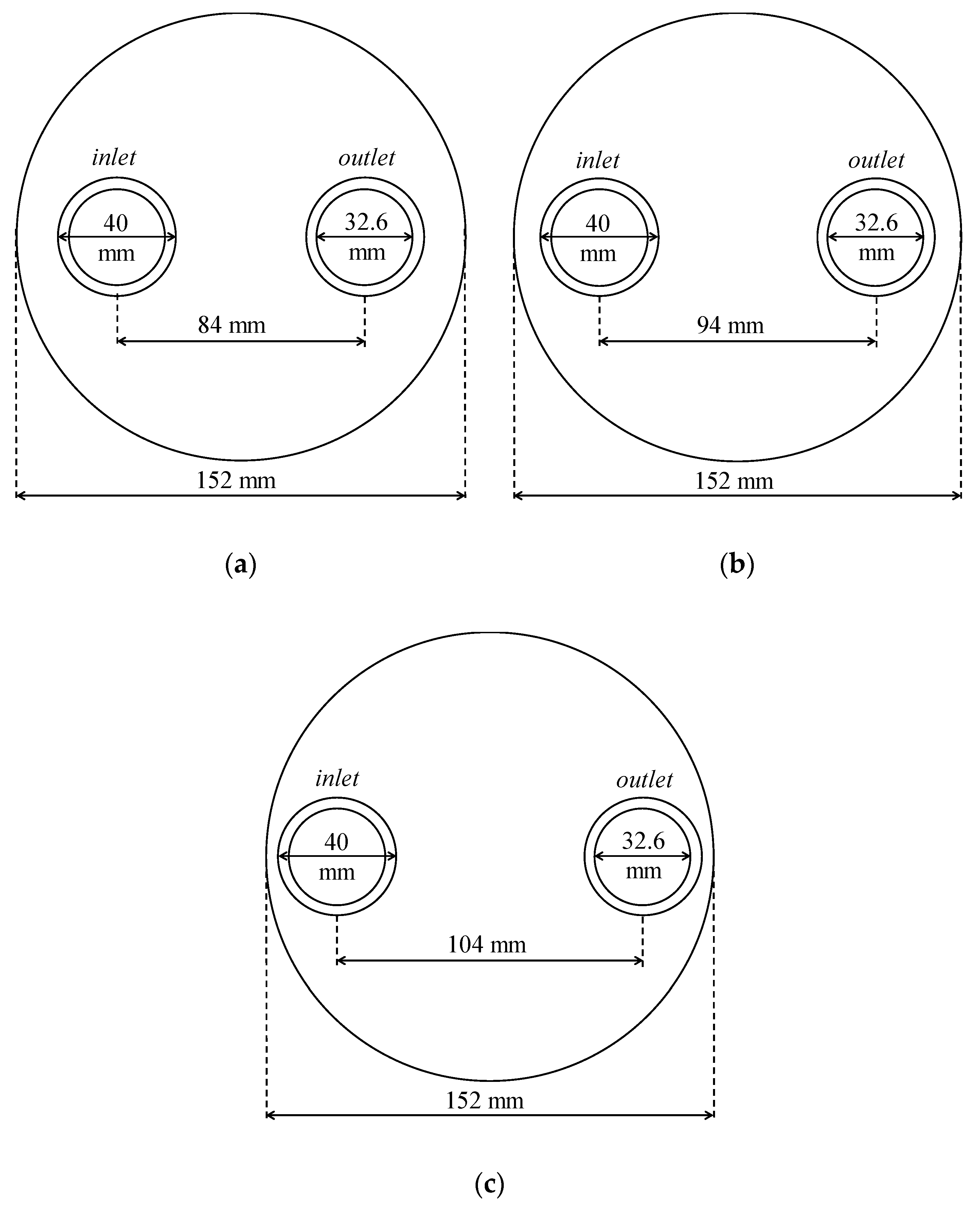
We considered nine BHE geometries, with BHE diameter D_b = 152 mm, shank spacing d = 84, 94 and 104 mm, length L = 50, 100 and 200 m, pipes with internal diameter D_pi = 32.6 mm and external diameter D_pe = 40 mm. Sketches of the BHE cross sections considered are illustrated in Figure 1.

For each geometry, we considered three grout thermal conductivities, 1.0, 1.6 and 2.3 W/(mK), two flow rates, $\dot{V}$ = 12 and 24 L/min, and ground thermal conductivity k_g = 1.8 W/(mK) (typical value). The following values were adopted for the thermal properties nearly uninfluential on φ: polyethylene thermal conductivity and volumetric heat capacity k_p = 0.4 W/(mK) and (ρ c)_p = 1.824 MJ/(m³K); grout and ground volumetric heat capacities (ρ c)_gt = 1.600 MJ/(m³K) and (ρ c)_g = 2.500 MJ/(m³K). We examined the cooling operation, with inlet fluid temperature 32 °C. Thus, 54 finite element simulations were performed to determine the correlations for φ. Additional simulations were performed to validate the simulation code, as well as to check the validity of the correlations for other values of D_b and of k_g and for other working conditions.

Water has been considered as working fluid. The water thermal properties at T_in have been taken from NIST [44]: density ρ_w = 995.03 kg/m³, dynamic viscosity μ_w = 0.76456 mPa s, specific heat capacity c_pw = 4179.5 J/(kg K), thermal conductivity k_w = 0.61869 W/(mK). The water velocity was considered vertical and uniform. A heat flux per unit area given by the product of the convection coefficient and the temperature difference between fluid and solid surface was applied at the fluid-solid interface. The Reynolds, Nusselt and Prandtl numbers, and the heat transfer coefficient h are given in

Table 1. Values of $\dot{V}$, of Re, Pr, and Nu numbers, and of the convection coefficient.

$\dot{\mathit{V}}$ (L/min)	Re	Pr	Nu	h (W/(m2K))
12	10,166	5.16	77.1	1462.2
24	20,332	5.16	135.5	2571.4

. The Nusselt number was calculated through the Churchill correlation with uniform wall heat flux [45].

The ground surrounding the borehole has been represented as a cylinder coaxial with the borehole, having radius 10 m and 10 m longer than the BHE. The initial temperature of the ground and of the BHE has been set equal to the undisturbed ground temperature, T_g. The latter has been supposed equal to 14 °C for z = 10 m, with geothermal gradient 0.03 °C/m for z > 10 m. The following distribution of T_g(z) has been assumed for z < 10 m:

$$T_g\left(z\right)=e^{-z}\times \left[T_g\left(0\right)-T_g\left(10\right)\right]+T_g\left(10\right),T_g\left(0\right)=24{}^{°}\mathrm{C}.$$

(7)

An adiabatic boundary condition has been imposed at the lateral and bottom ground surfaces and at the top of the borehole. The boundary condition T_g(0) = 24 °C has been applied at the horizontal ground surface.

Numerical simulations for a working period of 100 h have been carried out by a 3D finite element model, through COMSOL Multiphysics. The working period selected is more than sufficient to reach a quasi-stationary heat transfer regime in the BHE and to obtain abundant data of φ in this regime.

The reduced vertical coordinate $\tilde{z}=z/c$ has been introduced to shorten the computational domain along z [46]. Consequently, a reduced thermal conductivity along z, ${\tilde{k}}_z=k_z/c^2$, has been employed for every material; in addition, a reduced vertical water velocity $\tilde{w}=w/c$ has been assumed. A more detailed description of the method can be found in Refs. [43,46]. The reduction coefficient c has been taken equal to 5 for BHEs with length 50 m, equal to 10 for BHEs with length 100 m, and equal to 20 for BHEs with length 200 m.

In COMSOL Multiphysics, the time steps are non-uniform and are optimized by the software so that the solution matches the accuracy parameters imposed by the user. We have selected absolute tolerance 0.0001 and relative tolerance 0.001, instead of the default values 0.001 and 0.01, respectively.

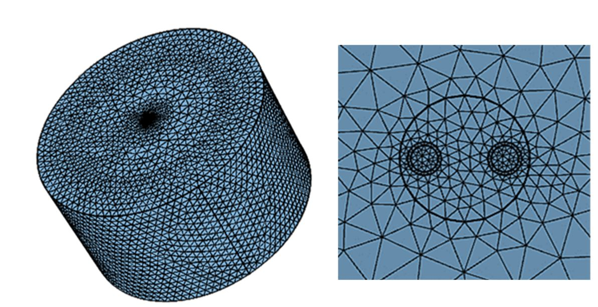
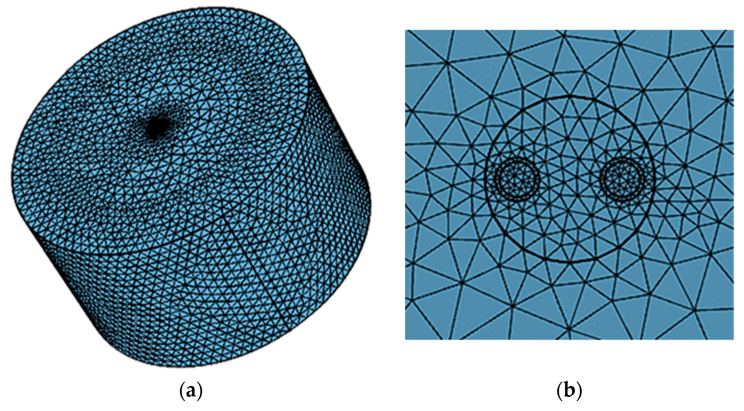
For each geometry, the computational domain has been meshed with unstructured tetrahedral elements. Due to the rescaling coefficient, the selected mesh, illustrated in Figure 2, is independent of the BHE length, and has 1,369,572 elements for d = 84 mm, 1,444,394 elements for d = 94 mm, and 1,510,647 elements for d = 104 mm.

In order to ensure that the results are mesh independent, simulations have been carried out by employing meshes with 1,198,027, 1,311,663 and 1,444,394 tetrahedral elements, for L = 100 m, d = 94 mm, k_gt = 1.6 W/(mK), k_g = 1.8 W/(mK), and $\dot{V}$ = 12 L/min. The values of T_ave − T_fm determined at τ = 2 h, 20 h and 100 h from the operation start have been compared, and the maximum percent deviation from the values obtained with the third mesh, employed in the final simulations, has been 0.127%.

3. Correlations for φ

The correlations for φ have been determined first for the quasi-stationary regime within the BHE, and then for the transient regime.

3.1. Quasi-Stationary Regime

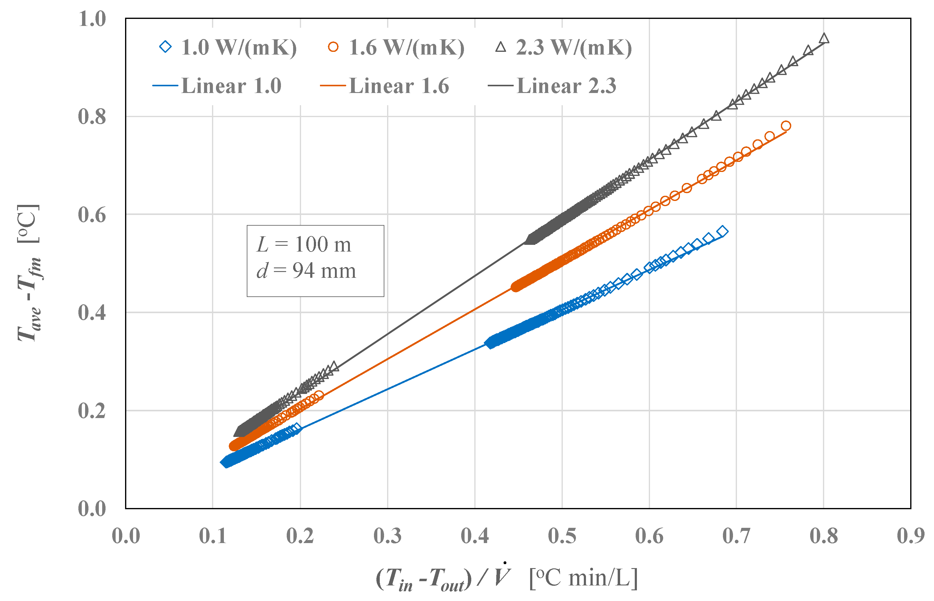
The simulation results revealed that, after 2 h of operation with constant T_in and $\dot{V}$, the quantity T_ave − T_fm becomes a homogeneous linear function of $\left(T_{in}-T_{out}\right)/\dot{V}$ that depends only on L, d, and k_gt. Thus, a homogeneous linear regression of T_ave − T_fm as a function of $\left(T_{in}-T_{out}\right)/\dot{V}$ has been determined for each BHE geometry and for each value of k_gt, by employing the simulation results for τ ≥ 2 h. The angular coefficient of each expression, divided by ${\dot{V}}_0$ = 12 L/min, gives a value of φ for the quasi-stationary regime, denoted by φ_∞. The linear regressions obtained for L = 100 m and d = 94 mm are illustrated, as an example, in Figure 3. The values of φ_∞ are reported in

Table 2. Values of φ_∞.

L (m)	d (mm)	kgt (W/(mK))	φ∞
50	84	1.0	0.0359
		1.6	0.0453
		2.3	0.0532
	94	1.0	0.0346
		1.6	0.0434
		2.3	0.0508
	104	1.0	0.0339
		1.6	0.0419
		2.3	0.0487
100	84	1.0	0.0700
		1.6	0.0884
		2.3	0.1035
	94	1.0	0.0676
		1.6	0.0847
		2.3	0.0989
	104	1.0	0.0662
		1.6	0.0817
		2.3	0.0950
200	84	1.0	0.1315
		1.6	0.1644
		2.3	0.1910
	94	1.0	0.1270
		1.6	0.1575
		2.3	0.1827
	104	1.0	0.1243
		1.6	0.1521
		2.3	0.1756

.

In order to determine a correlation for φ_∞, the following dimensionless quantities have been employed:

$$L^{*}=L/L_0,$$

(8)

$$k^{*}=k_{gt}/k_{gt0},$$

(9)

$$d^{*}=d/d_0,$$

(10)

where L₀ = 100 m, k_gt0 = 1.6 W/(mK), and d₀ = 94 mm are reference values of L, k_gt, and d. By employing these parameters, we obtained the correlation:

$${\phi }_{\infty }=0.043L^{*}+0.004684k^{*}/d^{*}+0.03109L^{*}{k}^{*}/d^{*}+0.00214.$$

(11)

Equation (11) can be employed to determine φ_∞, and therefore T_ave − T_fm and T_out − T_fm in quasi-stationary regime, for every single U-tube borehole with 50 m ≤ L ≤ 200 m, 84 mm ≤ d ≤ 104 mm, 1.0 W/(mK) ≤ k_gt ≤ 2.3 W/(mK). The mean square deviation of the values of φ_∞ given by Equation (11) from those reported in Table 2 is equal to 0.00237, i.e., to 2.51% of the mean value of φ_∞.

3.2. Transient Regime

The simulation results revealed that the time dependence of φ during the two first working hours can be fitted by the equation:

$$\phi ={\phi }_{\infty }\left(1+a{\mathrm{e}}^{-b{t}^{*}}\right),$$

(12)

where a and b are dimensionless coefficients dependent on L, d, k_gt and $\dot{V}$, and t^* is the dimensionless time, evaluated as the working time τ divided by two hours. Moreover, the dependence on L and $\dot{V}$ can be reduced to the dependence on the dimensionless parameter:

$$V^{*}=\dot{V}/\left({\dot{V}}_o{L}^{*}\right).$$

(13)

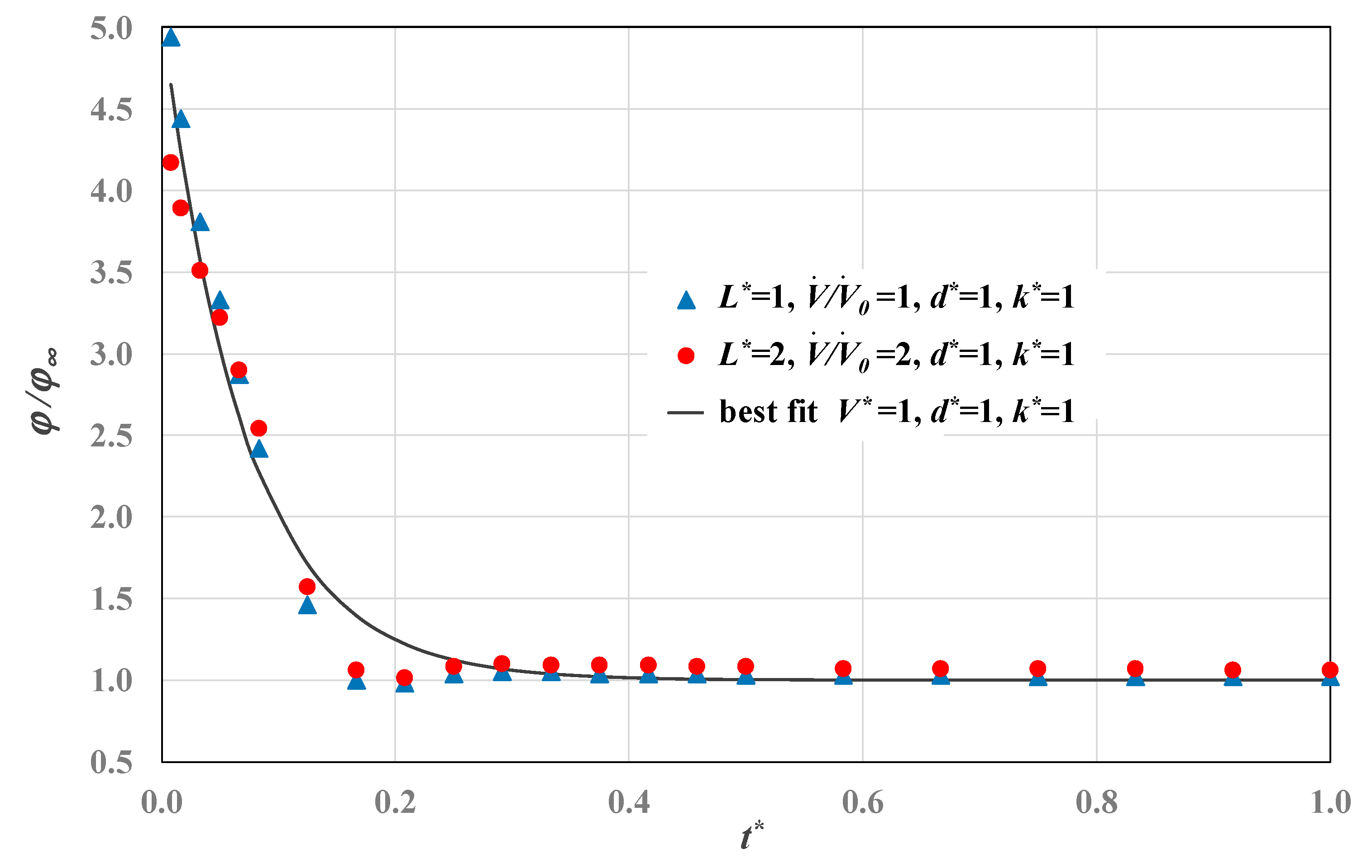
Four values of V^* were considered, namely 0.5, 1, 2 and 4. The coefficients a and b were determined by fitting values of φ/φ_∞ as a function of t^* obtained numerically. Figure 4 illustrates the best fit for V^* = 1, d^* = 1, k^* = 1, that was obtained through two simulations: with L^* = 1, $\dot{V}/{\dot{V}}_0=1$, d^* = 1, k^* = 1, and with L^* = 2, $\dot{V}/{\dot{V}}_0=2$, d^* = 1, k^*= 1. As shown by the figure, the best-fit curve yields very accurate values of φ/φ_∞, except for 0.125 < t^* < 0.25, where it slightly overestimates the simulation results.

The obtained values of a and b are listed in

Table 3. Values of a and b to be used in Equation (12).

V*	d*	k*	a	b
0.5	0.8936	0.625	1.8	7
		1	1.2	7
		1.4375	0.8	7
	1	0.625	1.9	7
		1	1.3	7
		1.4375	0.9	7
	1.1064	0.625	2	7
		1	1.4	7
		1.4375	1	7
1	0.8936	0.625	5.2	14
		1	3.9	14
		1.4375	3.2	14
	1	0.625	5.4	14
		1	4.1	14
		1.4375	3.4	14
	1.1064	0.625	5.6	14
		1	4.3	14
		1.4375	3.6	14
2	0.8936	0.625	15	42
		1	11.7	42
		1.4375	10	42
	1	0.625	15.5	42
		1	12.2	42
		1.4375	10.5	42
	1.1064	0.625	16	42
		1	12.7	42
		1.4375	11	42
4	0.8936	0.625	37	92
		1	29	92
		1.4375	25	92
	1	0.625	38	92
		1	30	92
		1.4375	26	92
	1.1064	0.625	39	92
		1	31	92
		1.4375	27	92

. As revealed by the table, a depends on V^*, d^*, and k^*, while b depends only on V^*. The correlation:

$$\begin{array}{l}a=\left(-0.0303V^{*}{}^2+2.5926V^{*}-0.47\right)d^{*}+\left(0.3423V^{*}{}^2+2.4718V^{*}-0.3486\right)k^{*}{}^2\\ –\left(0.9892V^{*}{}^2+7.744V^{*}-1.0553\right)k^{*}+1.1697V^{*}{}^2+8.7332V^{*}-2.3034\end{array}$$

(14)

fits the values of a given by Table 3 with a mean square deviation equal to 0.246.

The relative discrepancy between Equation (14) and Table 3 can be considered as negligible for values of a higher than 10.

The coefficient b, which depends only on V^*, can be expressed as:

$$b=0.6667V^{*}{}^2+21.8V^{*}-5.6667.$$

(15)

Equations (11), (12), (14) and (15) yield the time evolution of φ during the first two working hours, for every single U-tube BHE, in any working condition.

After the first hour of operation, the ratio φ/φ_∞ is very close to the asymptotic value 1. By integrating Equation (12) between t^* = 0 and t^* = 0.5 one obtains the mean value of φ during the first hour:

$${\phi }_{mean1}={\phi }_{\infty }\left[0.5+\frac{a}{b}\left(1-{\mathrm{e}}^{-0.5b}\right)\right].$$

(16)

4. Validation of the 3D Simulation Code

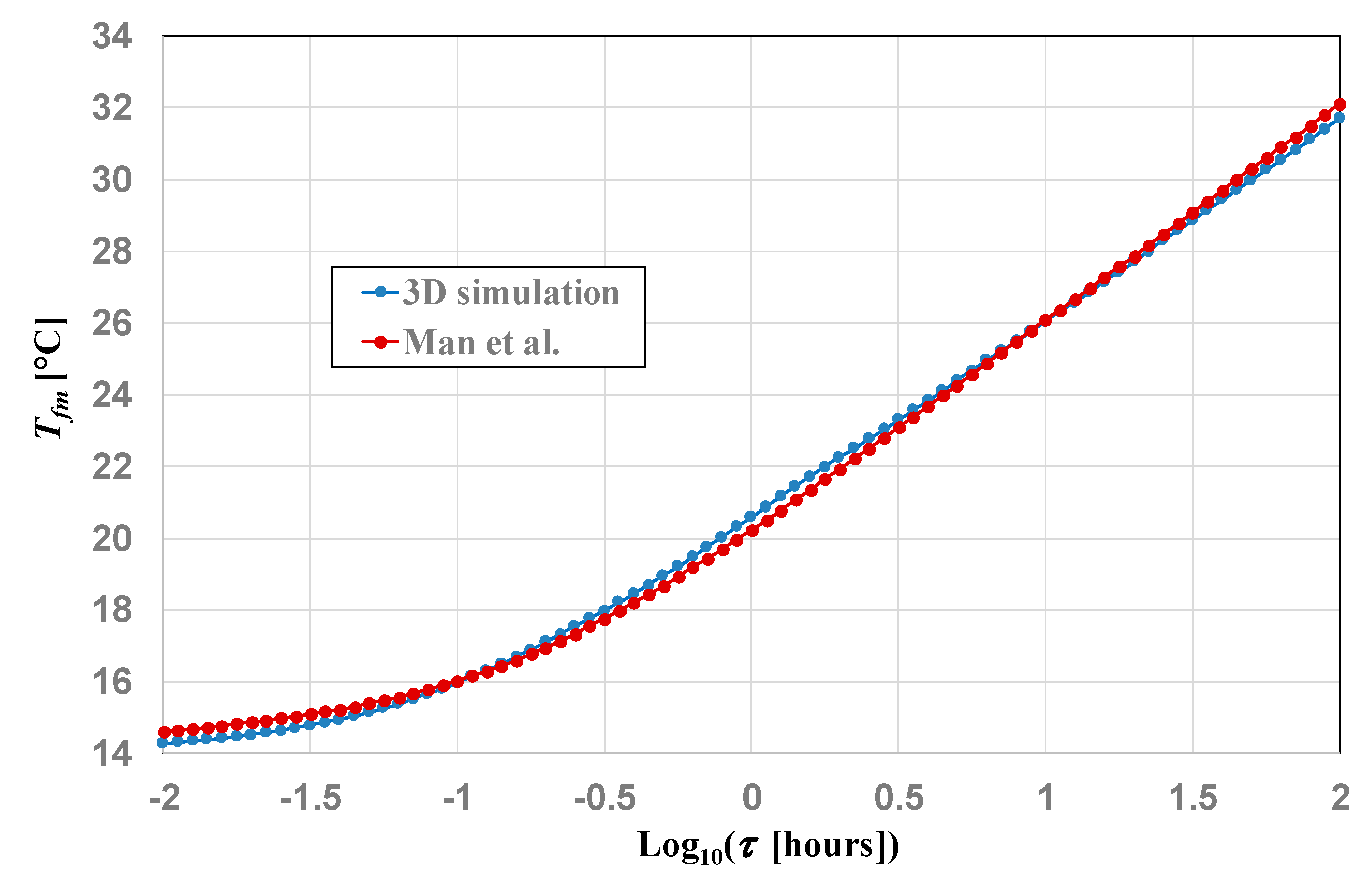
The validation of the 3D simulation code has been performed by comparison between the time-dependent values of T_fm evaluated through this code and those calculated analytically through the BHE model proposed by Man et al. [35]. The BHE selected for the comparison has L = 100 m, d = 94 mm, k_gt = 1.6 W/(mK), (ρ c)_gt = 1.600 MJ/(m³K), volume flow rate 18 L/min, is placed in a ground with k_g = 1.8 W/(mK) (ρ c)_g = 2.500 MJ/(m³K), T_g = 14 °C, and receives a time constant linear power of 60 W/m, i.e., to a total thermal power $\dot{Q}$ = 6000 W. The initial temperature coincides with T_g(z) in the whole domain. The properties of water are evaluated at 20 °C and are [44] ρ_w = 998.21 kg/m³, μ_w = 1.0016 mPa s, c_pw = 4184.1 J/(kg K), k_w = 0.59846 W/(mK). The convection coefficient, calculated by the Churchill correlation [45], is h = 1800.5 W/(m²K).

In the 3D simulation code, the condition of constant thermal power $\dot{Q}$ = 6000 W has been implemented by imposing the constant value of T_in − T_out given by Equation (3), namely 4.789 °C. The mesh is that illustrated in Figure 2.

In the 2D axisymmetric BHE model proposed by Man et al. [35], the BHE is represented by a cylindrical surface with radius r₀ that releases a constant and uniform power per unit area corresponding to the total thermal power received by the BHE. The generating surface represents the fluid, and the borehole has the same properties as the ground. The analytical solution for the temperature field is determined by the Green’s function method.

The mean temperature of the surface with radius r₀, that will be denoted by T_fm, is given by [35]:

$$\begin{array}{l}{T}_{fm}\left(\tau \right)=\frac{q_l}{8\pi k_{g}L}{\displaystyle \underset{0}{\overset{L}{\int }}\mathrm{d}z{\displaystyle \underset{0}{\overset{\tau }{\int }}d{\tau }^{\prime }\frac{1}{\tau -{\tau }^{\prime }}\times I_0\left[\frac{r_0^2}{2{\alpha }_g\left(\tau -{\tau }^{\prime }\right)}\right]}}\times \mathrm{Exp}\left[-\frac{r_0^2}{2{\alpha }_g\left(\tau -{\tau }^{\prime }\right)}\right]\\ \times \left\{\mathrm{Erf}\left[\frac{L-z}{2\sqrt{{\alpha }_g\left(\tau -{\tau }^{\prime }\right)}}\right]+2\mathrm{Erf}\left[\frac{z}{2\sqrt{{\alpha }_g\left(\tau -{\tau }^{\prime }\right)}}\right]-\mathrm{Erf}\left[\frac{L+z}{2\sqrt{{\alpha }_g\left(\tau -{\tau }^{\prime }\right)}}\right]\right\}+T_g\end{array}$$

(17)

where ${\alpha }_g=\left(k_g/{\left(\rho c\right)}_g\right)$ is the thermal diffusivity of the ground, equal to 0.72 × 10⁻⁶ m²/s in the case considered.

The value of r₀ to be employed in the model has been determined by imposing that the thermal resistance of the cylindrical layer between r₀ and the BHE radius is equal to the BHE thermal resistance. The latter has been determined through a stationary 2D finite element simulation of a borehole cross section that includes a ground layer having radius 2 m and an isothermal external surface. The temperature difference between the fluid and the external ground surface has been set equal to 25 °C for one pipe and to 20 °C for the other pipe. The convection coefficient is h = 1800.5 W/(m²K). We adopted a very fine mesh, composed of 139,008 triangular elements. A particular of the mesh employed is illustrated in Figure 5. The result is R_b = 0.09863 mK/W and, as a consequence, r₀ = 2.491 cm.

The diagrams of T_fm versus the decimal logarithm of time in hours obtained by the 3D finite element simulation and by the numerical integration of Equation (17) are compared in Figure 6, in the time range between 10⁻² h and 10² h. The mean square deviation between the results of the finite element simulation and those obtained by the model by Man et al. [35] is 0.26 °C. The small discrepancies that occur from 10⁻² to 10⁻¹ h are very probably due to the non-perfect accuracy of the analytical model, that does not consider the exact total value and distribution of the BHE heat capacity. On the contrary, those occurring from 10 to 10² h are probably due to numerical errors in the 3D simulation, that increase with time.

5. Validity of the Correlations for Other BHE Diameters, Thermal Conductivities of the Ground, Working Conditions

Although the correlations for φ reported in Section 3 were obtained by assuming D_b = 152 mm, k_g = 1.8 W/(mK), and summer operation with constant T_in, they hold also for other BHE diameters, ground thermal conductivities, and working conditions.

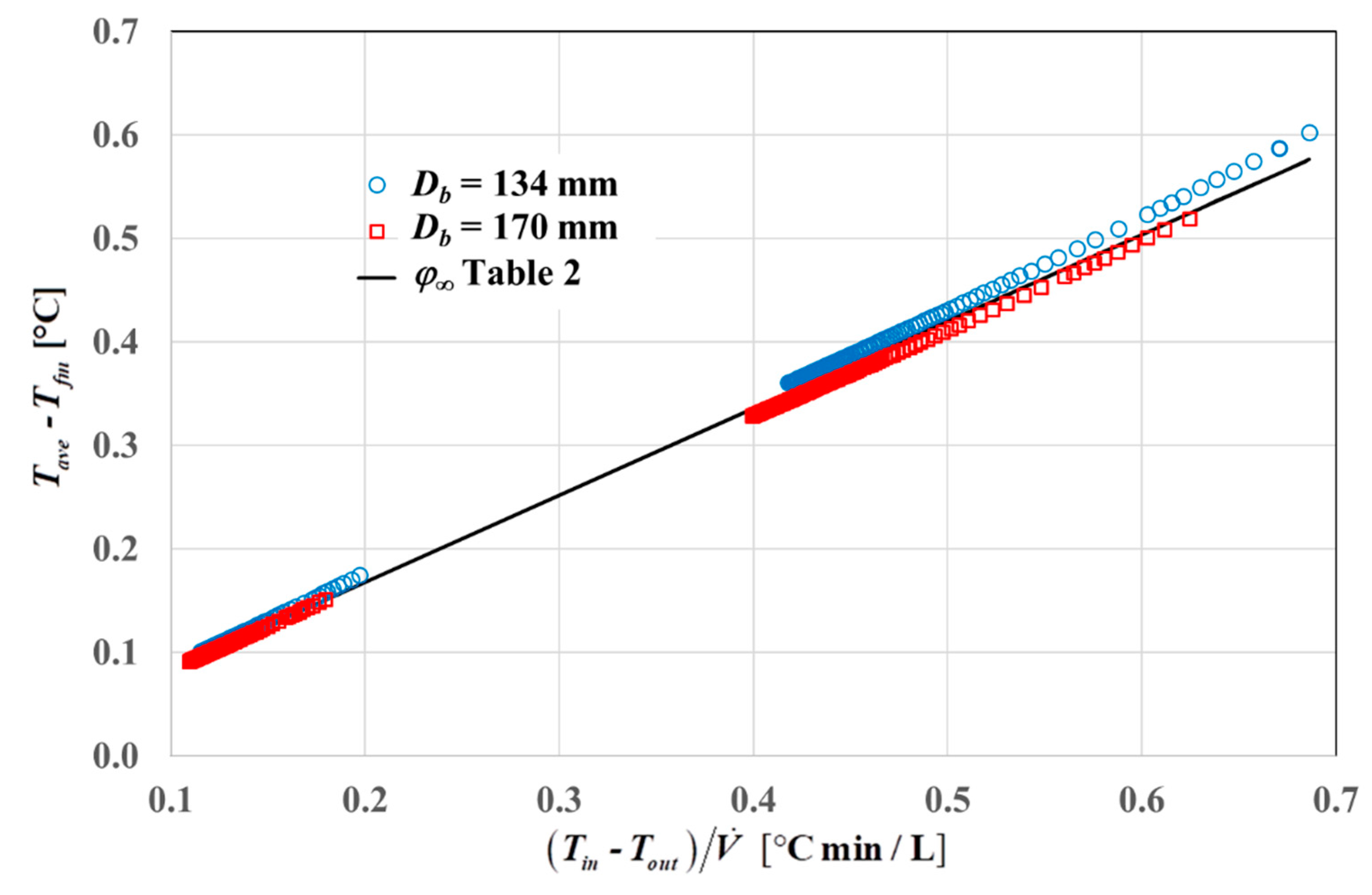
The applicability of the values of φ_∞ reported in Table 2 to other borehole diameters is shown in Figure 7, that refers to BHEs with L = 100 m, d = 84 mm, k_gt = 1.0 W/(mK), k_g = 1.8 W/(mK), $\dot{V}$ = 12 L/min, and BHE diameters 134 mm and 170 mm. Clearly, the value of D_b has no effect on φ if k_gt = k_g. Therefore, the value k_gt = 1.0 W/(mK) has been selected, to analyze a critical condition, with a high ratio k_g/k_gt. Higher values of this ratio should be avoided. The diagrams of T_ave − T_fm versus $\left(T_{in}-T_{out}\right)/\dot{V}$ obtained by the 3D simulations with these BHE diameters are compared with the line obtained by employing the value of φ_∞ reported in Table 2, namely φ_∞ = 0.07. The comparison shows the applicability of the correlation to other BHE diameters.

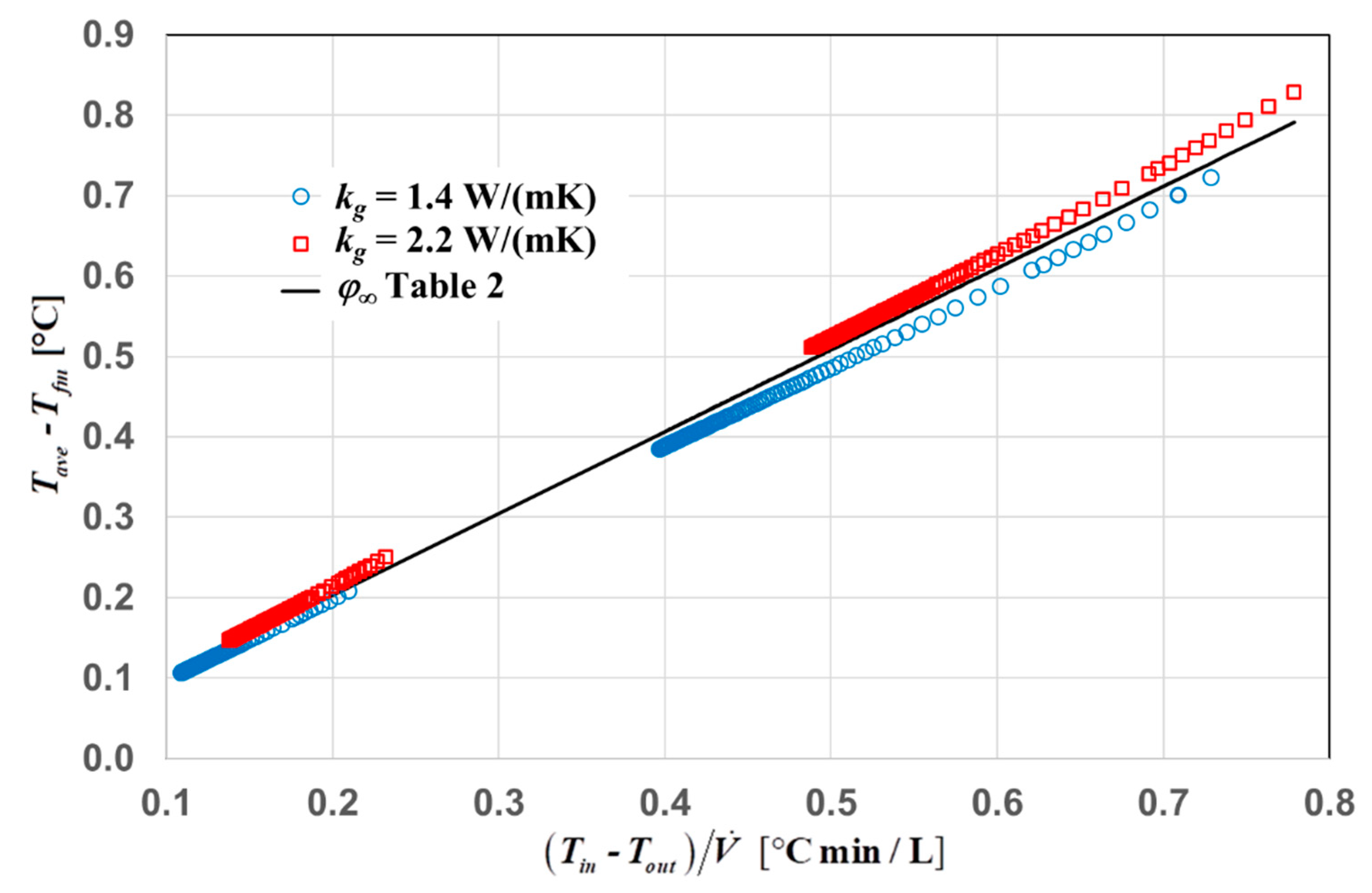
The applicability of the values of φ_∞ reported in Table 2 to other ground thermal conductivities is shown in Figure 8, that refers to BHEs with L = 100 m, d = 94 mm, k_gt = 1.6 W/(mK), $\dot{V}$ = 12 L/min, ground thermal conductivities 1.4 and 2.2 W/(mK). The diagrams of T_ave − T_fm versus $\left(T_{in}-T_{out}\right)/\dot{V}$ obtained by the 3D simulations with k_g = 1.4 and 2.2 W/(mK) are compared with the line obtained by employing the value of φ_∞ listed in Table 2, namely φ_∞ = 0.0847. The results reveal that the correlation can be applied to other values of the ground conductivity.

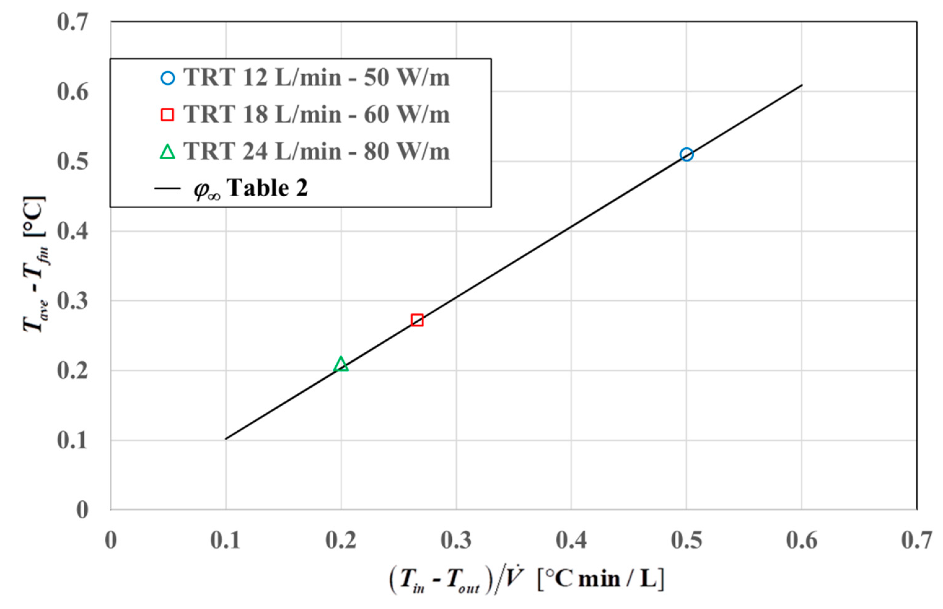
The applicability of the values of φ_∞ reported in Table 2 to other working conditions is shown in Figure 9, that refers to thermal response tests (TRTs) performed on a borehole with L = 100 m, d = 94 mm, k_gt = 1.6 W/(mK), k_g = 1.8 W/(mK). The working conditions are $\dot{V}$ = 12 L/min and q_l = 50 W/m for the first TRT, $\dot{V}$ = 18 L/min and q_l = 60 W/m for the second TRT, $\dot{V}$ = 24 L/min and q_l = 80 W/m for the third TRT. In a TRT, T_in − T_out is a constant and T_ave − T_fm becomes constant after 2 h. Therefore, only one value of T_ave − T_fm as a function of $\left(T_{in}-T_{out}\right)/\dot{V}$ is obtained for each TRT, in the quasi-stationary regime. In Figure 9, the values of T_ave − T_fm as a function of $\left(T_{in}-T_{out}\right)/\dot{V}$ obtained for the TRTs described above are compared with the line obtained by employing the value of φ_∞ reported in Table 2. The points that represent the results for the TRTs lay on the correlation line.

6. Evaluation of the Time Evolution of T_out by Means of the Correlations for φ

In this section, we show how the correlations for φ determined in Section 3 can be used to evaluate accurately T_out by means of simulation codes that yield T_fm, first in the case of constant heat load and flow rate, then in the case of time dependent heat load and constant flow rate. The accuracy obtainable in working conditions with time dependent flow rate is not analyzed in this paper.

6.1. Constant Heat Load

In this example, we determine T_fm by the analytical BHE model by Man et al. [35] and T_out by the correlations for φ, and we point out the errors that occur in the short time if one employs simpler methods, such as the finite line-source (FLS) model combined with either R_b or R_beff, or the model by Man et al. [35] without the correlations for φ.

Consider the same BHE as in Section 4 (L = 100 m, d = 94 mm, k_gt = 1.6 W/(mK), (ρ c)_gt = 1.600 MJ/(m³K), k_g = 1.8 W/(mK) (ρ c)_g = 2.500 MJ/(m³K), T_g = 14 °C), but with $\dot{V}$ = 12 L/min and q_l = 50 W/m (i.e., $\dot{Q}$ = 5000 W), as in the first TRT considered in Section 5. The water properties have the same values as in Section 4. The convection coefficient is h = 1303.8 W/(m²K) [45]. The BHE thermal resistance, determined by a 2D steady state simulation by the method explained in Section 4, is R_b = 0.09965 mK/W. The effective BHE thermal resistance has been determined by Hellström’s analytical expression [47]:

$$R_{b,eff}=R_b\eta \coth \eta ,$$

(18)

where:

$$\eta =\frac{L}{\dot{m}{c}_p\sqrt{R_a{R}_b}}$$

(19)

and R_a is the internal resistance between the tubes. The latter has been evaluated through the expression [48]:

$$R_a=\frac{2\left(T_{f1}-T_{f2}\right)}{q_{l1}-q_{l2}},$$

(20)

where T_f1 and T_f2 are the bulk temperatures in the tubes, and q_l1 and q_l2 are the heat fluxes per unit length from the tubes. The results obtained are R_a = 0.47555 mK/W, R_b,eff = 0.10950 mK/W.

In the model of Ref. [35], the radius of the generating surface such that the thermal resistance of the cylindrical layer between that surface and the BHE radius equals R_b is r₀ = 2.462 cm.

The simplest method to obtain the time evolution of T_out is determining T_sm by the FLS model and T_fm by Equation (1), then adopting the approximation:

T_fm ≈ T_ave

(21)

and evaluating T_out by the relation:

$$T_{out}=T_{ave}-0.5\frac{\dot{Q}}{\dot{m}{c}_p}.$$

(22)

An improvement of this method is determining T_sm by the FLS model, T_ave by the definition of effective BHE thermal resistance:

$$T_{ave}-T_{sm}=q_{lm}{R}_{b,eff},$$

(23)

and then T_out by Equation (22). This improvement allows obtaining correct values of T_out in the long term.

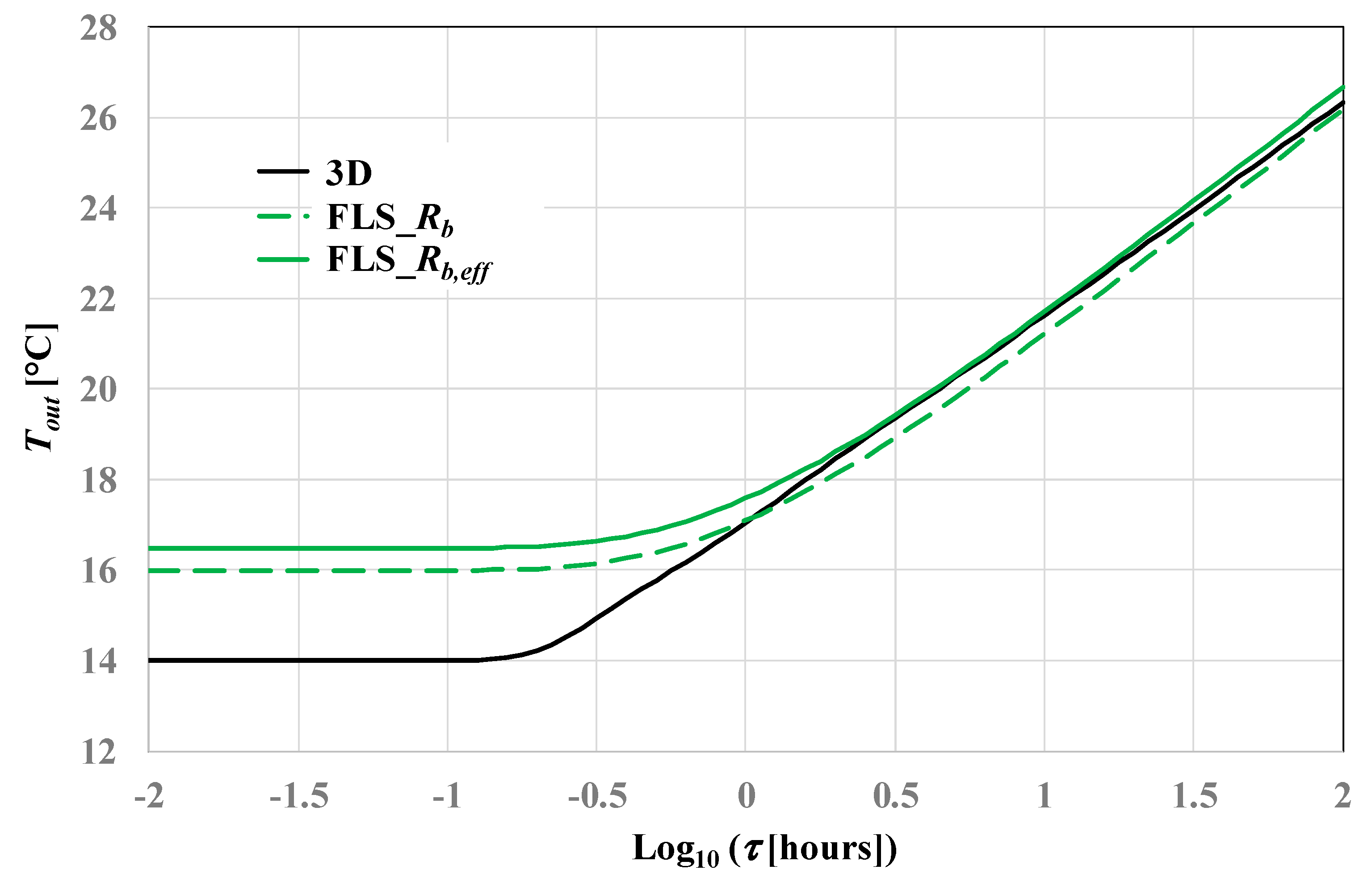
The time evolution of T_out obtained by applying the FLS model and R_b and that obtained by applying the FLS model and R_b,eff are compared in Figure 10 with that obtained by a 3D finite element simulation performed by the method described in Section 2 and the grid illustrated in Figure 2. The time interval considered is from 10⁻² h to 10² h, in the logarithmic scale.

The time evolution of T_sm by the FLS model has been obtained through the numerical integration of the expression determined by Bandos et al. [15]:

$$T_{sm}\left(\tau \right)=\frac{q_l}{4\pi k_g}{\displaystyle \underset{r_b/\sqrt{4{\alpha }_g\tau }}{\overset{\infty }{\int }}\left\{4\mathrm{Erf}\left(\frac{Lu}{r_b}\right)-2\mathrm{Erf}\left(\frac{2Lu}{r_b}\right)-\left(3+{\mathrm{e}}^{-4L^2{u}^2/r_b^2}-4{\mathrm{e}}^{-L^2{u}^2/r_b^2}\right)\frac{r_b}{\sqrt{\pi }Lu}\right\}}\frac{{\mathrm{e}}^{-u^2}}{u}\mathrm{d}u.$$

(24)

The figure shows that the methods based on the FLS model yield an important overestimation of T_out during the first hour. In fact, while the true value of T_out remains practically equal to 14 °C during the first ten minutes, T_out jumps immediately from 14 to 16 °C according to the FLS_R_b method, and from 14 to 16.48 °C according to the FLS_R_b,eff method, that is more accurate in the long term. The overestimation of T_out by the FLS_R_b,eff method starts decreasing after 10 min, but remains relevant for about one hour (0.76 °C for τ = 1 h).

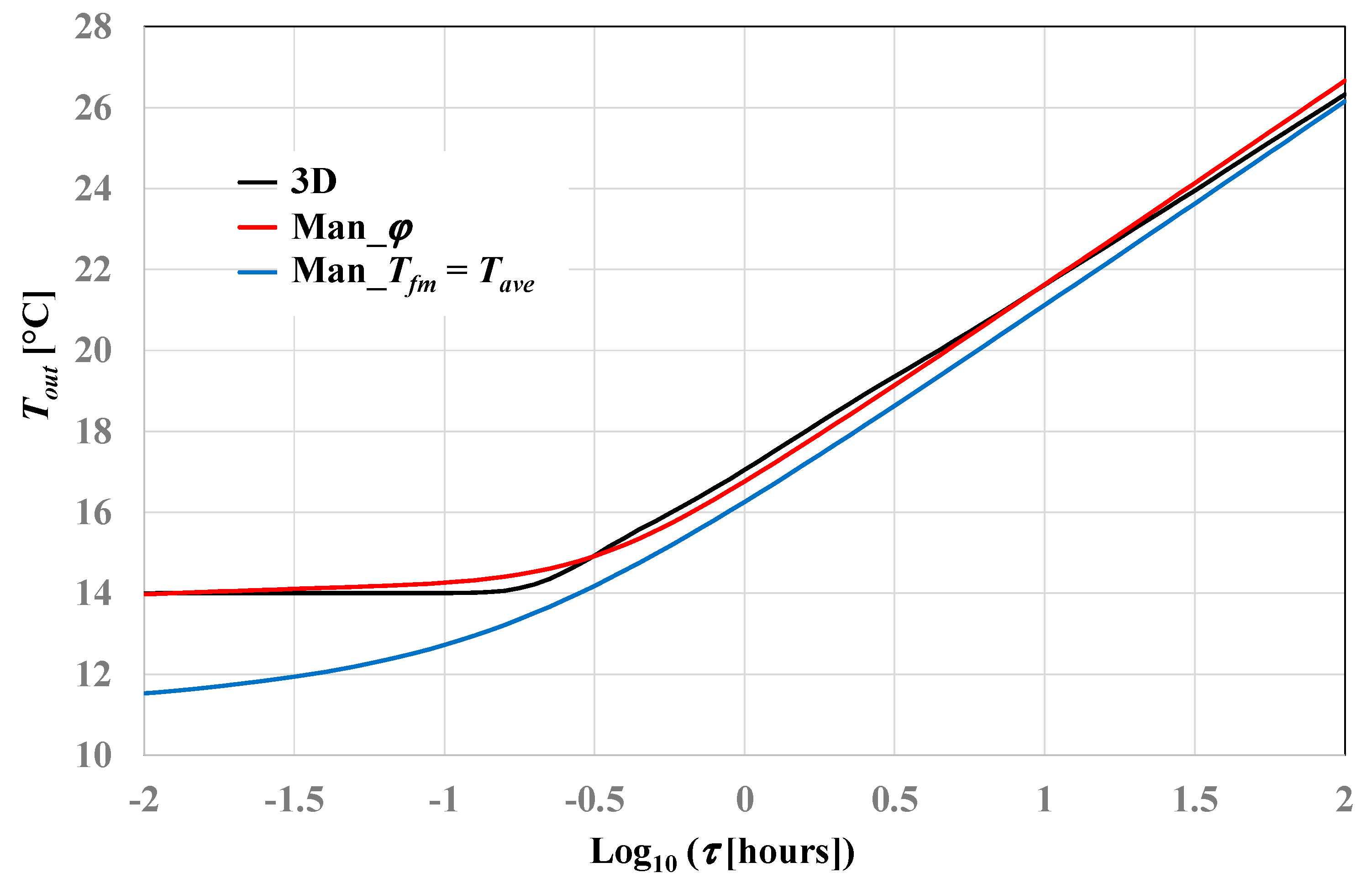
A much more accurate evaluation of the time evolution of T_out can be obtained by determining the time evolution of T_fm by means of a full-time scale BHE model that takes into account the heat capacity of the borehole elements, and calculating T_out through the coefficient φ and Equation (6). The time evolution of T_out yielded by the model of Ref. [35] and the coefficient φ is compared with that obtained by the 3D finite element simulation described above in Figure 11. The time dependent value of φ has been determined through Equation (12), with the value of φ_∞ given in Table 2 (0.0847) and the values of a and b given in Table 3 (4.1 and 14, respectively). The figure shows that the combined use of the model by Man et al. [35] and of the coefficient φ yields results in fair agreement with those of the 3D numerical simulation, even for very short times.

Figure 11 illustrates also the results obtained by employing the model of Ref. [35] coupled with the approximation T_fm ≈ T_ave and Equation (22), and shows that the approximate method underestimates T_out in the short time.

6.2. Time Dependent Heat Load

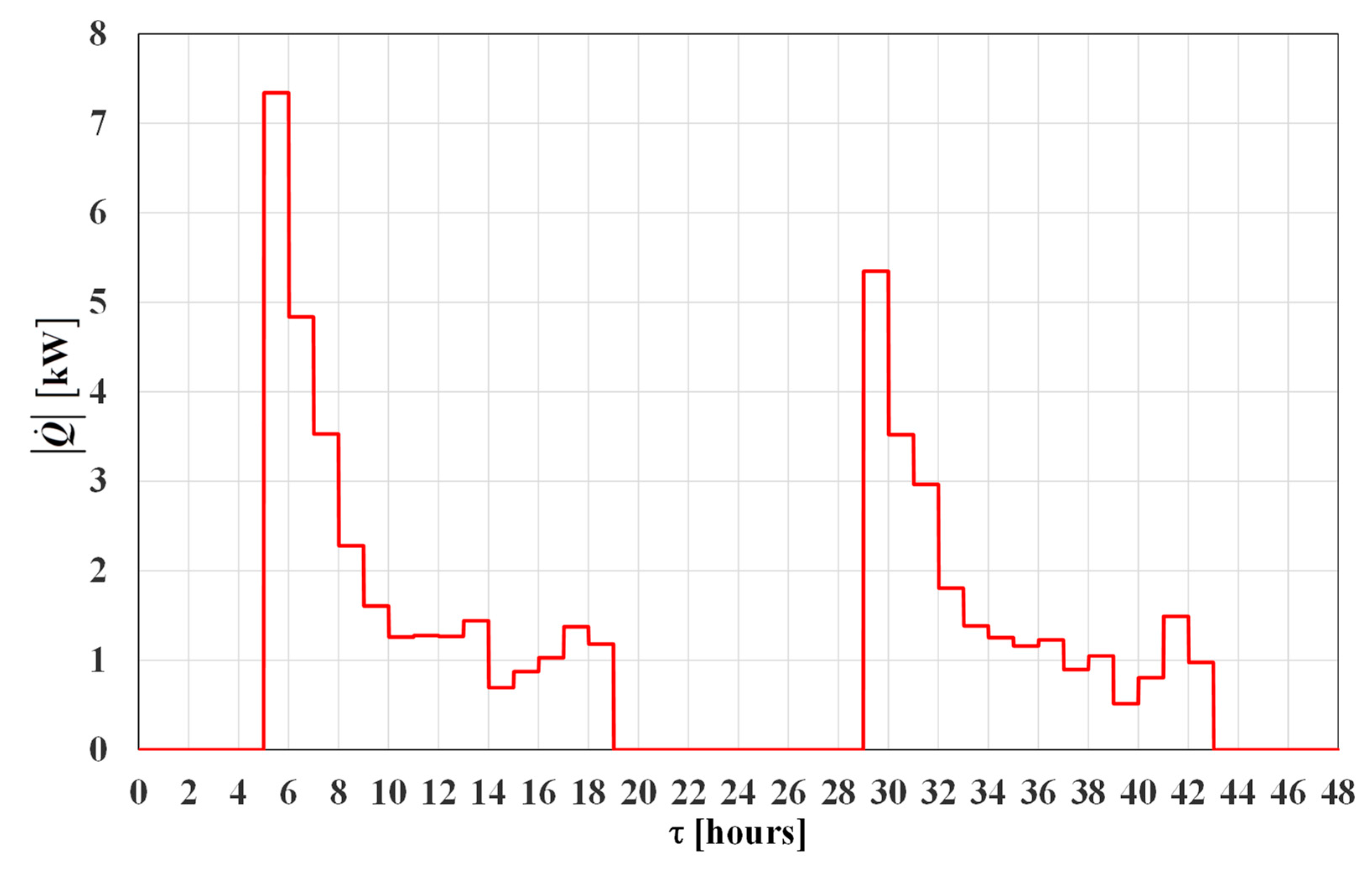
We illustrate now the use of our correlation for φ to determine T_out in the case of a heat load with sharp step changes. We consider the hourly demand of thermal energy of an uninsulated office building located in Bologna (Italy), during the first two days of the heating period, namely October 15 and 16, of a typical meteorological year. The building has two floors and a heated floor area of 1255.7 m². Heating is turned on at 5 a.m. and is turned off at 7 p.m. The hourly values of the thermal energy required by the building, including the distribution and emission heat losses, have been determined by a dynamic simulation performed through TRNSYS 17. In our example, we assume that the building is heated by a heat pump with COP = 4, coupled with 12 BHEs, each 100 m long, and determine the hourly heat loads on each BHE multiplying by 0.75 and dividing by 12 the hourly values of the total thermal energy required by the building. A dynamic simulation of the building-plant system with values of the heat pump COP determined at each hour is beyond the aims of this paper. The absolute values of the negative hourly heat load on each BHE are illustrated in Figure 12.

The absolute values of $\dot{Q}$ during the first five hours are 7.341, 4.835, 3.527, 2.278, 1.606 kW, respectively, and the absolute value of the mean heat load during the first 24 h is 1.249 kW. We consider the same BHE, the same flow rate, and the same initial and boundary conditions as in Section 6.1, with the only difference that the thermal properties of water are evaluated at 11 °C, and are [44] ρ_w = 999.61 kg/m³, μ_w = 1.2691 mPa s, c_pw = 4193.6 J/(kg K), k_w = 0.58193 W/(mK), and the convection coefficient is [45] h = 1172.3 W/(m²K).

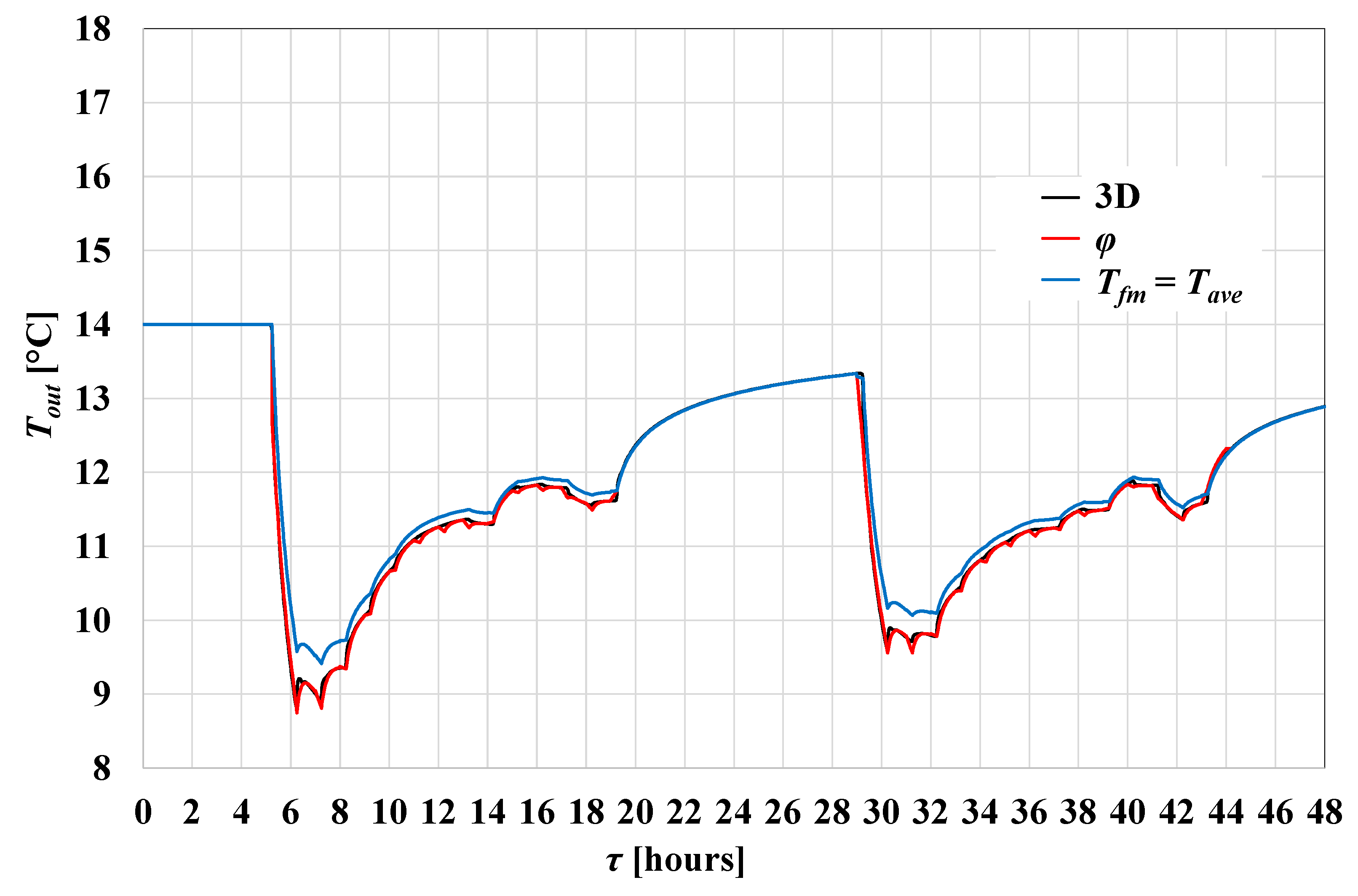
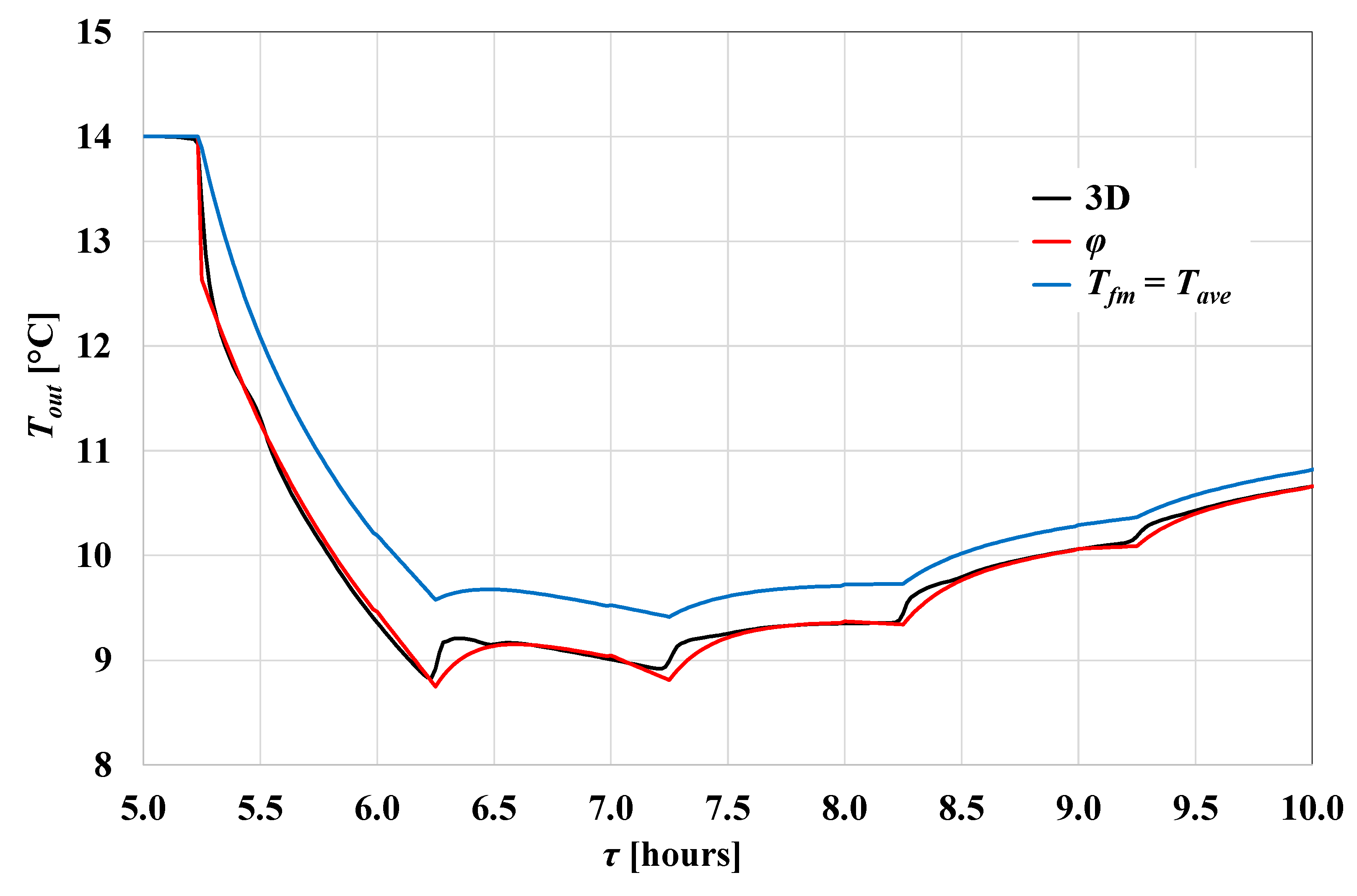
The time evolutions of T_fm and of T_out are determined by a 3D finite element simulation of the BHE, performed by the same simulation code and the same mesh as in Section 6.1. Then, the time evolution of T_out is calculated from that of T_fm by means of our correlations for φ and Equation (6), with the following method. The time interval Δt needed by the fluid to go from the inlet to the outlet is evaluated by assuming plug flow, i.e., a uniform velocity in each cross section: 14 min for the case considered. For each hour, the dimensionless time t^* of Equation (12) starts from zero at the beginning of the hour, and the application of the correlations for φ starts after a time interval Δt from the beginning of the hour. During the time interval Δt of the first hour, T_out is kept constant with the same value as in the initial instant, as is physically consistent and confirmed by the 3D simulation. During the time interval Δt of any other hour, T_out is considered as linearly varying with time from the last time instant of the preceding hour to the first time instant after Δt of that hour. A comparison between the time evolution of T_out yielded by the 3D simulation and that obtained through our correlation for φ is illustrated in Figure 13, and a particular for the first five hours is illustrated in Figure 14. The figures report also the time evolution of T_out that is obtained by employing the same method to manage the initial time interval Δt of each hour, and by applying the customary approximation T_fm = T_ave instead of the correlations for φ.

The figures show that the time evolution of T_out obtained by applying the correlations for φ is much more accurate, especially during the most critical hours. The mean square deviation from the results of the 3D simulation, during the first three hours, is 0.1 °C for the method employing our correlations for φ and 0.6 °C for that employing the approximation T_fm = T_ave.

7. Calculation of R_b,eff Through φ_∞

In this section we show that, in quasi-stationary working conditions, the effective BHE thermal resistance, R_b,eff, can be easily calculated by means of the dimensionless coefficient φ_∞. Then, we compare the values of R_b,eff evaluated through our general correlation for φ_∞, given by Equation (11), with those determined by 3D finite element computations and by Hellström’s analytical solution.

One can rewrite Equation (23) as:

$$R_{b,eff}=\frac{T_{ave}-T_{sm}}{q_{lm}}=\frac{T_{ave}-T_{fm}}{q_{lm}}+\frac{T_{fm}-T_{sm}}{q_{lm}}=\frac{T_{ave}-T_{fm}}{q_{lm}}+R_b.$$

(25)

In quasi-stationary working conditions, the energy balance of the fluid yields:

$$q_{lm}=\frac{\dot{m}{c}_p\left(T_{in}-T_{out}\right)}{L}.$$

(26)

By substituting Equation (26) in Equation (25), one gets:

$$R_{b,eff}=R_b+\frac{T_{ave}-T_{fm}}{T_{in}-T_{out}}\frac{L}{\dot{m}{c}_p}.$$

(27)

In quasi-stationary conditions, Equation (5) yields:

$$\frac{T_{ave}-T_{fm}}{T_{in}-T_{out}}=\frac{{\dot{V}}_0}{\dot{V}}{\phi }_{\infty }.$$

(28)

By substituting Equation (28) in Equation (27), one obtains:

$$R_{b,eff}=R_b+\frac{{\dot{V}}_0}{\dot{V}}\frac{{\phi }_{\infty }L}{\dot{m}{c}_p}.$$

(29)

Equations (29) and (11) allow a very simple calculation of the difference between R_b,eff and R_b, for single U-tube BHEs. Equation (29) can be employed also in combination with Equation (27) of Ref. [43], for double U-tube BHEs. The BHE thermal resistance R_b can be calculated either by employing a suitable approximate expression, or, more accurately, through a 2D numerical simulation of a borehole cross section.

A comparison between the values of R_b,eff obtained by Equations (29) and (11), denoted by R_b,eff,φ, those evaluated through 3D numerical computations, denoted by R_b,eff,3D, and those obtained by Equations (18) and (19), denoted by R_b,eff,H, is illustrated in

Table 4. Values of R_b,eff,φ, R_b,eff,3D, and R_b,eff,H, for D_b = 152 mm, k_g = 1.8 W/(mK), T_in = 32 °C, $\dot{V}$ = 12 L/min, and different values of d, L and k_gt.

d (mm)	L (m)	kgt (W/(mK))	Rb,eff,φ (mK/W)	Rb,eff,3D (mK/W)	Rb,eff,H (mK/W)
84	100	1.0	0.1469	0.1472	0.1467
		1.6	0.1152	0.1159	0.1154
		2.3	0.0998	0.1001	0.0995
	200	1.0	0.1709	0.1711	0.1705
		1.6	0.1442	0.1457	0.1444
		2.3	0.1345	0.1348	0.1324
94	100	1.0	0.1364	0.1368	0.1362
		1.6	0.1090	0.1097	0.1092
		2.3	0.0953	0.0958	0.0953
	200	1.0	0.1595	0.1598	0.1592
		1.6	0.1365	0.1382	0.1369
		2.3	0.1280	0.1289	0.1267
104	100	1.0	0.1260	0.1267	0.1260
		1.6	0.1033	0.1041	0.1036
		2.3	0.0916	0.0922	0.0916
	200	1.0	0.1484	0.1491	0.1483
		1.6	0.1297	0.1316	0.1303
		2.3	0.1226	0.1240	0.1217

, for single U-tube BHEs having L = 100 m or 200 m, D_b = 152 mm, k_g = 1.8 W/(mK), $\dot{V}$ = 12 L/min and inlet temperature T_in = 32 °C. The convection coefficient is h = 1462.2 W/(m²K), as indicated in Table 1. The values of R_a and of R_b to be employed in Equations (18) and (19) have been determined by performing stationary 2D numerical simulations of a borehole cross section with the method described in Section 4 and evaluating R_a with Equation (20).

The table shows that the values of R_b,eff evaluated through our correlation for φ_∞ are in fair agreement both with those computed directly by 3D numerical computations and with those yielded by Hellström’s analytical method. The highest percent deviation from R_b,eff,3D is −1.46% for R_b,eff,φ and −1.81% for R_b,eff,H; the mean square deviation from R_b,eff,3D is 0.00093 mK/W for R_b,eff,φ and 0.00119 mK/W for R_b,eff,H.

The values of R_b,eff,φ reported in Table 4 have been determined by calculating φ_∞ through Equation (11). If one employs the values of φ_∞ reported in Table 2, the highest percent deviation from R_b,eff,3D reduces to −1.05% and the mean square deviation reduces to 0.00086 mK/W.

8. Conclusions

By means of 3D finite element simulations of single U-tube borehole heat exchangers (BHEs), we have obtained simple expressions of a dimensionless coefficient φ that yields two temperature differences: that between the average of inlet and outlet fluid temperature, T_ave, and the mean fluid temperature, T_fm; that between the outlet temperature, T_out, and T_fm. The obtained expressions of φ hold for single U-tube BHEs with any diameter between 130 and 170 mm, any shank spacing compatible with the diameter, and any BHE length between 50 m and 200 m, both in quasi-stationary and in transient regime. The 3D simulation code has been validated by comparing the time evolution of T_fm obtained by the code with that obtained by applying an analytical BHE model.

We have shown that the obtained expressions of φ allow an accurate evaluation of the time evolution of T_out through a BHE model that yields the time evolution of T_fm, for working conditions with constant flow rate and either constant or time dependent heat load. Moreover, we have illustrated the errors that occur in the short time if one applies the finite line-source model coupled with the effective BHE thermal resistance, and those that occur if one applies a BHE model that yields T_fm coupled with the approximation T_fm = T_ave. Thus, the obtained expressions of φ are a useful complement of the BHE models that yield T_fm. Finally, we have shown that the obtained quasi-stationary values of φ can be used for a simple evaluation of the effective BHE thermal resistance.

References

- Lund, J.W.; Boyd, T.L. Direct Utilization of Geothermal Energy 2015 worldwide review. Geothermics 2016, 60, 66–93. [Google Scholar] [CrossRef]
- Spitler, J.D.; Gehlin, S. Measured Performance of a Mixed-Use Commercial-Building Ground Source Heat Pump System in Sweden. Energies 2019, 12, 2020. [Google Scholar] [CrossRef] [Green Version]
- Li, M.; Zhou, C.; Rao, Z. Hourly 50-year simulations of ground-coupled heat pumps using high-resolution analytical models. Energy Convers. Manag. 2019, 193, 15–24. [Google Scholar] [CrossRef]
- Rivoire, M.; Casasso, A.; Piga, B.; Sethi, R. Assessment of Energetic, Economic and Environmental Performance of Ground-Coupled Heat Pumps. Energies 2018, 11, 1941. [Google Scholar] [CrossRef] [Green Version]
- Naldi, C.; Zanchini, E. Effects of the total borehole length and of the heat pump inverter on the performance of a ground-coupled heat pump system. Appl. Therm. Eng. 2018, 128, 306–319. [Google Scholar] [CrossRef]
- Ruiz-Calvo, F.; Montagud, C.; Cazorla-Marín, A.; Corberán, J.M. Development and Experimental Validation of a TRNSYS Dynamic Tool for Design and Energy Optimization of Ground Source Heat Pump Systems. Energies 2017, 10, 1510. [Google Scholar] [CrossRef] [Green Version]
- Jung, Y.-J.; Kim, H.-J.; Choi, B.-E.; Jo, J.-H.; Cho, Y.-H. A Study on the Efficiency Improvement of Multi-Geothermal Heat Pump Systems in Korea Using Coefficient of Performance. Energies 2016, 9, 356. [Google Scholar] [CrossRef] [Green Version]
- Kavanaugh, S.P.; Rafferty, K. Ground-Source Heat Pumps. Design of Geothermal Systems for Commercial and Institutional Buildings; ASHRAE: Atlanta, GA, USA, 1997. [Google Scholar]
- Hellström, G.; Sanner, B. EED—Earth Energy Designer, Version 1.0, User’s Manual; Knoblich & Partner GmbH: Wetzlar, Germany, 1997. [Google Scholar]
- Spitler, J.D. GLHEPRO—A design tool for commercial building ground loop heat exchanger. In Proceedings of the 4th International Conference on Heat Pumps in Cold Climates, Aylmer, QC, Canada, 17–18 August 2000; pp. 1–16. [Google Scholar]
- Fisher, D.E.; Rees, S.J.; Padhmanabhanc, S.K.; Murugappan, A. Implementation and validation of ground-source heat pump system models in an integrated building and system simulation environment. HvacR Res. 2006, 12, 693–710. [Google Scholar] [CrossRef]
- ASHRAE Handbook, HVAC Applications; ASHRAE: Atlanta, GA, USA, 2015; Chapter 34.
- Claesson, J.; Eskilson, P. Conductive Heat Extraction by a Deep Borehole, Analytical Studies; Technical Report; Lund University: Lund, Sweden, 1987. [Google Scholar]
- Zeng, H.Y.; Diao, N.R.; Fang, Z.H. A finite line-source model for boreholes in geothermal heat exchangers. Heat Transf. Asian Res. 2002, 31, 558–567. [Google Scholar] [CrossRef]
- Bandos, T.V.; Montero, A.; Fernandez, E.; Santander, J.L.G.; Isidro, J.M.; Perez, J.; Fernandez de Cordoba, P.J.; Urchueguia, J.F. Finite line-source model for borehole heat exchangers: Effect of vertical temperature variations. Geothermics 2009, 38, 263–270. [Google Scholar] [CrossRef]
- Zanchini, E.; Lazzari, S. Temperature distribution in a field of long borehole heat exchangers (BHEs) subjected to a monthly averaged heat flux. Energy 2013, 59, 570–580. [Google Scholar] [CrossRef]
- Puttige, A.R.; Rodriguez, J.; Monzó, P.; Cerdeira, F.; Fernandez, A.; Novelle, L.; Acuña, J.; Mogensen, P. Improvements on a Numerical Model of Borehole Heat Exchangers; European Geothermal Congress: Strasbourg, France, 2016; p. 10. [Google Scholar]
- Cimmino, M.; Bernier, M. A semi-analytical method to generate g-functions for geothermal bore fields. Int. J. Heat Mass Transf. 2014, 70, 641–650. [Google Scholar] [CrossRef]
- Monzó, P.; Mogensen, P.; Acuña, J.; Ruiz-Calvo, F.; Montagud, C. A novel numerical approach for imposing a temperature boundary condition at the borehole wall in borehole fields. Geothermics 2015, 56, 35–44. [Google Scholar] [CrossRef]
- Priarone, A.; Fossa, M. Temperature response factors at different boundary conditions for modelling the single borehole heat exchanger. Appl. Therm. Eng. 2016, 103, 934–944. [Google Scholar] [CrossRef]
- Naldi, C.; Zanchini, E. A new numerical method to determine isothermal g-functions of borehole heat exchanger fields. Geothermics 2019, 77, 278–287. [Google Scholar] [CrossRef]
- Cimmino, M. The effects of borehole thermal resistances and fluid flow rate on the g-functions of geothermal bore fields. Int. J. Heat Mass Transf. 2015, 91, 1119–1127. [Google Scholar] [CrossRef]
- Monzó, P.; Puttige, A.R.; Acuña, J.; Mogensen, P.; Cazorla, A.; Rodriguez, J.; Montagud, C.; Cerdeira, F. Numerical modeling of ground thermal response with borehole heat exchangers connected in parallel. Energy Build. 2018, 172, 371–384. [Google Scholar] [CrossRef] [Green Version]
- De Carli, M.; Tonon, M.; Zarrella, A.; Zecchin, R. A computational capacity resistance model (CaRM) for vertical ground-coupled heat exchangers. Renew. Energy 2010, 35, 1537–1550. [Google Scholar] [CrossRef]
- Zarrella, A.; Scarpa, M.; De Carli, M. Short time step analysis of vertical ground-coupled heat exchangers: The approach of CaRM. Renew. Energy 2011, 36, 2357–2367. [Google Scholar] [CrossRef]
- Quaggiotto, D.; Zarrella, A.; Emmi, G.; De Carli, M.; Pockelé, L.; Vercruysse, J.; Psyk, M.; Righini, D.; Galgaro, A.; Mendrinos, D.; et al. Simulation-Based Comparison Between the Thermal Behavior of Coaxial and Double U-Tube Borehole Heat Exchangers. Energies 2019, 12, 2321. [Google Scholar] [CrossRef] [Green Version]
- Bauer, D.; Heidemann, W.; Muller-Steinhagen, H.; Diersch, H.-J.G. Thermal resistance and capacity models for borehole heat exchangers. Int. J. Energy Res. 2011, 35, 312–320. [Google Scholar] [CrossRef]
- Pasquier, P.; Marcotte, D. Short-term simulation of ground heat exchanger with an improved TRCM. Renew. Energy 2012, 46, 92–99. [Google Scholar] [CrossRef]
- Ruiz-Calvo, F.; De Rosa, M.; Acuña, J.; Corberán, J.M.; Montagud, C. Experimental validation of a short-term Borehole-to-Ground (B2G) dynamic model. Appl. Energy 2015, 140, 210–223. [Google Scholar] [CrossRef] [Green Version]
- Li, M.; Lai, A.C.K. New temperature response functions (G functions) for pile and borehole ground heat exchangers based on composite-medium line-source theory. Energy 2012, 38, 255–263. [Google Scholar] [CrossRef]
- Li, M.; Lai, A.C.K. Analytical model for short-time responses of ground heat exchangers with U-shaped tubes: Model development and validation. Appl. Energy 2013, 104, 510–516. [Google Scholar] [CrossRef]
- Zhang, L.; Zhang, Q.; Huang, G. A transient quasi-3D entire time scale line source model for the fluid and ground temperature prediction of vertical ground heat exchangers (GHEs). Appl. Energy 2016, 170, 65–75. [Google Scholar] [CrossRef]
- Beier, R.A.; Smith, M.D. Minimum duration of in-situ tests on vertical boreholes. ASHRAE Trans. 2003, 109, 475–486. [Google Scholar]
- Xu, X.; Spitler, J.D. Modeling of vertical ground loop heat exchangers with variable convective resistance and thermal mass of the fluid. In Proceedings of the 10th International Conference on Thermal Energy Storage, Ecostock 2006, Pomona, NJ, USA, 31 May–2 June 2006. [Google Scholar]
- Man, Y.; Yang, H.; Diao, N.; Liu, J.; Fang, Z. A new model and analytical solutions for borehole and pile ground heat exchangers. Int. J. Heat Mass Transf. 2010, 53, 2593–2601. [Google Scholar] [CrossRef]
- Bandyopadhyay, G.; Gosnold, W.; Mann, M. Analytical and semi-analytical solutions for short-time transient response of ground heat exchangers. Energy Build. 2008, 40, 1816–1824. [Google Scholar] [CrossRef]
- Javed, S.; Claesson, J. New analytical and numerical solutions for the short-term analysis of vertical ground heat exchangers. ASHRAE Trans. 2011, 117, 3–12. [Google Scholar]
- Claesson, J.; Javed, S. An analytical method to calculate borehole fluid temperatures for time-scales from minutes to decades. ASHRAE Trans. 2011, 117, 279–288. [Google Scholar]
- Beier, R.A. Transient heat transfer in a U-tube borehole heat exchanger. Appl. Therm. Eng. 2014, 62, 256–266. [Google Scholar] [CrossRef]
- Lamarche, L. Short-time analysis of vertical boreholes, new analytic solutions and choice of equivalent radius. Int. J. Heat Mass Transf. 2015, 91, 800–807. [Google Scholar] [CrossRef]
- Naldi, C.; Zanchini, E. Full-Time-Scale Fluid-to-Ground Thermal Response of a Borefield with Uniform Fluid Temperature. Energies 2019, 12, 3750. [Google Scholar] [CrossRef] [Green Version]
- Beier, R.A.; Spitler, J.D. Weighted average of inlet and outlet temperatures in borehole heat exchangers. Appl. Energy 2016, 174, 118–129. [Google Scholar] [CrossRef]
- Zanchini, E.; Jahanbin, A. Simple equations to evaluate the mean fluid temperature of double U-tube borehole heat exchangers. Appl. Energy 2018, 231, 320–330. [Google Scholar] [CrossRef]
- NIST Chemistry WebBook. Available online: https://webbook.nist.gov/chemistry/fluid/ (accessed on 18 December 2019).
- Churchill, S.W. Comprehensive correlating equations for heat, mass and momentum transfer in fully developed flow in smooth tubes. Ind. Eng. Chem. Fundam. 1977, 16, 109–116. [Google Scholar] [CrossRef]
- Zanchini, E.; Lazzari, S.; Priarone, A. Improving the thermal performance of coaxial borehole heat exchangers. Energy 2010, 35, 657–666. [Google Scholar] [CrossRef]
- Hellström, G. Ground Heat Storage; Thermal Analysis of Duct Storage Systems. Ph.D. Thesis, Department of Mathematical Physics, University of Lund, Lund, Sweden, 1991. [Google Scholar]
- Lamarche, L.; Kajl, S.; Beauchamp, B. A review of methods to evaluate borehole thermal resistances in geothermal heat-pump systems. Geothermics 2010, 39, 187–200. [Google Scholar] [CrossRef]
Figure 1.
Sketches of the BHE cross sections considered, with shank spacing 84 mm (a), 94 mm (b) and 104 mm (c).
Figure 2.
Illustration of the mesh employed for d = 94 mm (a), and particular of the borehole top (b).
Figure 3.
Linear regressions of Tave − Tfm as a function of , for L = 100 m, d = 94 mm, kgt = 1.0, 1.6 and 2.3 W/(mK).
Figure 4.
Best fit of the simulation results of φ/φ∞ versus t* for V* = 1, d* = 1, k* = 1.
Figure 5.
Particular of the mesh adopted to determine Rb, for the validation of the 3D simulation code. The boundary between the polyethylene pipes and the grout is hidden by the triangular elements.
Figure 6.
Comparison of the time evolution of Tfm evaluated numerically and that determined through the analytical model by Man et al. [35].
Figure 7.
Diagrams of Tave − Tfm versus obtained by 3D simulations, for Db = 134 mm and Db = 170 mm, and by the value of φ∞ reported in Table 2.
Figure 8.
Diagrams of Tave − Tfm versus obtained by 3D simulations, for kg = 1.4 W/(mK) and kg = 2.2 W/(mK), and by the value of φ∞ reported in Table 2.
Figure 9.
Values of Tave − Tfm versus obtained for TRTs, compared with the correlation given by the value of φ∞ reported in Table 2.
Figure 10.
Time evolutions of Tout obtained by a 3D numerical simulation (3D), by the FLS model and Rb (FLS_Rb), and by the FLS model and Rb,eff (FLS_Rb,eff): constant heat load.
Figure 11.
Time evolutions of Tout obtained by a 3D numerical simulation (3D), by the model of Ref. [35] and our correlations for φ (Man_φ), and by the model of Ref. [35] and the approximation Tfm = Tave (Man_Tfm = Tave): constant heat load.
Figure 12.
Absolute values of the hourly heat load on each BHE, in kW, corresponding to the heating demand of an office building in Bologna during October 15 and 16 of a typical meteorological year.
Figure 13.
Time evolutions of Tout obtained by a 3D numerical simulation (3D), by Tfm and our correlations for φ (φ), and by Tfm and the approximation Tfm = Tave (Tfm = Tave): time dependent heat load.
Figure 14.
Time evolutions of Tout obtained by a 3D numerical simulation (3D), by Tfm and our correlations for φ (φ), and by Tfm and the approximation Tfm = Tave (Tfm = Tave): time dependent heat load, first 5 h.