1
School of Engineering and Science, Jacobs University Bremen, Bremen, Germany
2
Institut des Hautes Études Scientifiques, Bures-sur-Yvette, France
3
UniversitÉ Pierre et Marie Curie, Paris, France
In a recent publication (Müller-Linow et al., 2008
) two types of correlations between network topology and dynamics have been observed: waves propagating from central nodes and module-based synchronization. Remarkably, the dynamic behavior of hierarchical modular networks can switch from one of these modes to the other as the level of spontaneous network activation changes. Here we attempt to capture the origin of this switching behavior in a mean-field model as well in a formalism, where excitation waves are regarded as avalanches on the graph.
The question, how network architecture systematically shapes dynamic processes on the network, has become one of the key topics of research in a range of disciplines – from systems biology (Barabási and Oltvai, 2004
; Alon, 2007
; Brandman and Meyer, 2008
) and ecology (Uchida et al., 2007
) to logistics (Armbruster et al., 2005
; Guimera et al., 2005
) and sociology (Kearns et al., 2006
). In neuroscience this question is of particular importance, as functional properties of the brain can be expected to emerge from the organization of (essentially excitable) dynamics on the network of neurons.
Network research employs the formal view of graph theory to understand the design principles of complex systems. For many biological and technical networks, a large-scale system-wide perspective of the network architecture (the ‘topology’ of such graphs) has yielded some unexpected universal features, e.g., the ubiquitousness of heavy-tail degree distributions (Barabási and Albert, 1999
; Barabási and Oltvai, 2004
), the presence and possible functions of modularity in enhancing the robustness of a network and in organizing network tasks (Ravasz et al., 2002
; Guimera and Amaral, 2005
) and a similarity in motif content of functionally similar networks (Milo et al., 2004
; Alon, 2007
), where motifs are groups of few nodes with a specific link pattern.
Discrete dynamics, and in particular binary and three-state dynamics, have proven helpful in the past for studying, how dynamical processes depend on graph topology (Bornholdt, 2005
; Marr and Hütt, 2005
; Müller-Linow et al., 2006
; Drossel, 2008
).
Here we follow this line of thought and study the interplay of topology and dynamics for an important class of dynamical processes, namely excitable dynamics currently used as a minimal model of neuron firing, and for an important graph class, namely hierarchical networks. A hierarchical organization is an important feature of many complex networks in biology. Recently, synchronization on hierarchical networks has been studied (Arenas et al., 2006
, 2008
). In particular, it has been shown that the hierarchical levels of nodes in the network prescribe a cascade-like sequence toward a fully synchronized state (Arenas et al., 2006
).
In general, the shaping of dynamic processes by network topology can also be characterized as a correlation between network properties and properties of the dynamics (Müller-Linow et al., 2008
). Qualitatively speaking, a dynamic process typically groups statistically identical nodes into different functional categories. Understanding the impact of the network topology on the functioning of a dynamic process therefore starts by explaining the topological systematics of these node categories induced by the dynamical process.
Within the simple model of excitable dynamics on graphs, which we also use here (see Materials and Methods), two types of correlation between network topology and dynamics have been analyzed by numerical simulation: waves propagating from central nodes and module-based synchronization (Müller-Linow et al., 2008
). These two dynamic regimes represent a graph-equivalent to classical spatiotemporal pattern formation.
In order to quantify such modes of pattern formation, one can analyze properties of the matrix of simultaneous excitations, which for example can be studied using a clustering analysis. When analyzing these dynamics on a modular graph, the clusters obtained from the matrix of simultaneous excitations coincide well with the topological modules of the graph. Similarly, when analyzing the dynamics on a scalefree graph, the clusters essentially match groups of nodes with the same distance to the main hub of the graph.
Surprisingly, certain networks, e.g. hierarchical modular networks, contain enough topological cues for allowing both types of patterns to emerge: The dynamic behavior of such networks can switch from one of these modes to the other as the level of spontaneous node activation increases (Müller-Linow et al., 2008
).
Here we attempt to understand this switching behavior analytically using a combination of mean-field techniques with the notion of an effective network accessible to excitation.
In Section ‘Materials and Methods’ we briefly describe the hierarchical network model we use and the model of excitable dynamics, together with a short summary of previous results obtained within the same model. In Section ‘Results’ we first reproduce the findings from Müller-Linow et al. (2008)
in a simpler context, then we discuss the failure of the straightforward mean-field as well as pair-correlation descriptions to account for the organization of the dynamics on graphs (see Materials and Methods). A suitable incorporation of graph topology into a mean-field framework is proposed with the notion of effective networks, which at each moment in time are accessible to the dynamics due to an interplay of spontaneous activity and recovery rate. Excitation patterns can then be viewed as avalanches comprising the accessible effective network. This avalanche model is described in Section ‘Results’.
Network Architecture
A hierarchical system is intuitively defined by a multi-layered organization, where few top-level elements are related to several elements on intermediate levels, which are in turn related to a large number of bottom-level elements. Several parameterizations and generative rules of hierarchical graphs coexist in the literature. Typical variants rely on a modules-within-modules view (Ravasz et al., 2002
; Kaiser et al., 2007
), others focus on the coexistence of modules and central nodes (hubs) (Han et al., 2004
; Guimera and Amaral, 2005
) or relate the concept of hierarchies to fractality (Sporns, 2006
).
Even though our formalism is applicable to any network, here we analyze a specific model of hierarchical graphs, namely the one introduced by Ravasz et al. (2002) and Ravasz and Barabási (2003)
. In each iteration step four copies of the current network are set up and interlinked in a specific pattern: the central node is linked to all outside nodes; then the local hubs are interlinked among themselves (see Figures 1 and 2
). The first iteration step leads to four fully connected nodes. At the fourth iteration, the network has N = 256 nodes linked by 780 edges, parted in 4 shells according to their distance from the hub, containing respectively S0 = khub = 120, S1 = 54, S2 = 72 and S3 = 9 nodes.
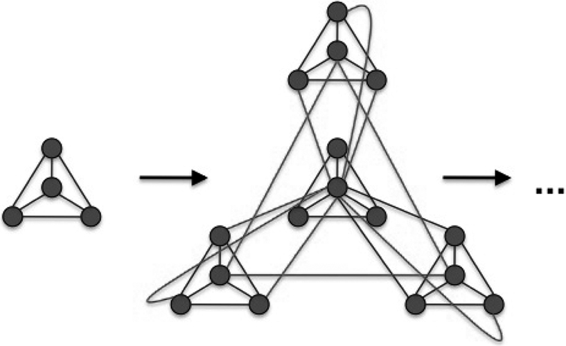
Figure 1. Iteration step in the recursive construction of the hierarchical graphs from Ravasz et al. (2002) and Ravasz and Barabási (2003)
.
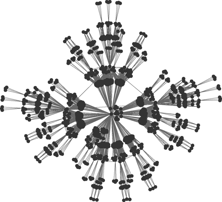
Figure 2. Hierarchical graph with N = 1024 nodes obtained from the iterative scheme described in Ravasz et al. (2002) and sketched on Figure 1
.
Dynamics
For discussing the link between topology and dynamics we use a simple three-state model of an excitable medium. The model consists of three discrete states for each node (susceptible s, excited e, refractory r), which are updated synchronously in discrete time steps according to the following rules: (1) A susceptible node becomes an excited node, if there is at least one excited node in its direct neighborhood. If not, spontaneous firing occurs with the probability f , which is the rate of spontaneous excitation; (2) an excited node enters the refractory state; (3) a node regenerates with the recovery probability p (the inverse of which is the average refractory time of a node). This minimal model of an excitable system has a rich history in biological modeling. It has been first introduced in a simpler variant under the name ‘forest fire model’ (Bak et al., 1990
) and subsequently expanded by Drossel and Schwabl (1992)
who also introduced the rate of spontaneous excitation (the ‘lightning probability’ in their terminology). In this form it was originally applied on regular architectures in studies of self-organized criticality. Other variants of three-state excitable dynamics have been used to describe epidemic spreading (see, e.g., Bailey, 1975
; Anderson and May, 1991
; Hethcote, 2000
; Moreno et al., 2002
) or to investigate the impact of topology on the dynamics (Carvunis et al., 2006
). Note that in Carvunis et al. (2006)
the recovery is deterministic (p = 1) and there is no spontaneous excitation (f = 0). In contrast, there is no refractory state in the SIS model of epidemic spreading, and no recovery (p = 0) in the SIR model (Pastor-Satorras and Vespignani, 2004
). As discussed previously (Graham and Matthai, 2003
; Müller-Linow et al., 2006
), this general model can readily be implemented on arbitrary network architectures. In Graham and Matthai (2003)
it has been shown that short-cuts inserted into a regular (e.g., ring-like) architecture can mimic the dynamic effect of spontaneous excitation. Using a similar model setup we have shown (Müller-Linow et al., 2006
) that the distribution pattern of excitations is regulated by the connectivity as well as by the rate of spontaneous excitations. An increase of either of the two quantities leads to a sudden increase in the excitation density accompanied by a drastic change in the distribution pattern from a collective, synchronous firing of a large number of nodes in the graph (spikes) to more local, long-lasting and propagating excitation patterns (bursts). Further studies on the activity of integrate-and-fire neurons in the classical small-world model from Watts and Strogatz (1998
) also revealed a distinct dependency of the dynamic behavior on the connectivity of the system (Roxin et al., 2004
).
In order to study the pattern of joint excitations on a hierarchical graph, we consider for all nodes the individual time series describing their successive states and for each pair of nodes (i, j) compute the number Cij of simultaneous firing events. When applied to the whole network the resulting matrix C (which in the following will be called the similarity matrix, as it captures the similarity of time series of two nodes) essentially represents the distribution pattern of excitations. This pattern can now be compared with a corresponding distribution pattern of some topological property.
Previous numerical studies (Müller-Linow et al., 2008
) have shown that different topological features of complex networks, such as node centrality and modularity, organize the synchronized network function at different levels of spontaneous activity. These findings serve as a starting point of our investigation.
Correlations of the Similarity Matrix with Graph Topology
In Müller-Linow et al. (2008)
clustering trees derived from the matrix of simultaneous excitations (the similarity matrix C) have been compared with groups of nodes derived from topological properties. These properties are modularity and node centrality and they have been represented by a topological-modularity-based reference and a central-node-based reference, respectively. Here we analyze the correlations more directly by comparing the similarity matrix C with matrices designed to capture the topological feature of interest, because the quantities introduced by Müller-Linow et al. (2008)
, while suitable for experimental studies of dynamics on graphs, have no direct analytical counterpart.
Two topological features are discussed here: (i) modularity, represented by the topological overlap matrix (Ravasz et al., 2002
) Tij = (Nij + Aij)/min (ki,kj), where Nij is the number of common neighbors of nodes i and j, A is the graph’s adjacency matrix and ki is the degree of node i; (ii) the distance di of node i from the graph’s central hub; for comparison with the similarity matrix C this distance is cast into a matrix D, where Dij = 1, if nodes i and j have the same distance to the hub and Dij = 0 otherwise.
As a measure of correlation of two matrices (where one typically is the similarity matrix and the other one of the matrices derived from topology) we use the mutual information M (m(1),m(2)) of the two binary matrices m(1) and m(2):
where pab denotes the relative frequency of encountering the element a in matrix m(1) and b at the same position in matrix m(2)(with a,b = 1,0) and  is the relative frequency of a in matrix m(k). An alternative quantification is the correlation coefficient Corr (m(1),m(2)) of the two matrices:
is the relative frequency of a in matrix m(k). An alternative quantification is the correlation coefficient Corr (m(1),m(2)) of the two matrices:
where av (m(k)) and σ (m(k)) denote the average and standard deviation over all values in matrix m(k), respectively. However, neither for the topological case nor for a typical similarity matrix at intermediate f the distribution of matrix elements follows a Gaussian distribution, so that mutual information better captures the correlation than the correlation coefficient Corr. It should be noted that the quantitative comparison of graphs (and matrices derived from graphs) is, in itself, a broad area of research. Distances between graphs can differ in the topological feature they emphasize or the length scale(s) considered. One alternative to the correlation coefficient and the mutual information used here could be the spectral distance method from Ipsen and Mikhailov (2002)
. Here we preferred the other two methods, because the dynamics are not directly coupled to spectral features (although this in itself may be an interesting investigation).
Figure 3
shows the correlation of the similarity matrix with the two matrices derived from topology, namely T (measuring modularity; full curves) and D (measuring similarity in their distance to the hub; dashed curves) as a function of the rate of spontaneous excitations f. These curves reproduce the finding from Müller-Linow et al. (2008)
: at low f the distribution of excitations is predominantly explained by ring structures around the hub (CN, central node reference), while at higher f the distribution becomes dominated by the modular structure of the graph (TM, topological module reference).
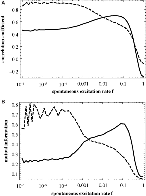
Figure 3. Correlation between the similarity matrix C(f) and the topological matrices T (full curve) and D (dashed curve) as a function of f for the hierarchical graph with N = 256 nodes. The correlation is measured (A) by the correlation coefficient of the two matrices, Eq. 2, and (B) by the mutual information, Eq. 1.
It should be noted that these results differ from Müller-Linow et al. (2008
, Figure 8A), because in Müller-Linow et al. (2008)
a sparser graph has been used in order to keep the average number of excitations at a comparable level for all the graphs discussed there (see Methods section in Müller-Linow et al., 2008
for a detailed description of this procedure). Here we wanted to use the original graph from Ravasz et al. (2002)
instead. Figure 4
shows the same mutual information curves as in Figure 3
B, but with the 1024-node network depicted in Figure 2
. With increasing network size the two patterns seem to become more pronounced. In both cases, Figures 3 and 4
, the two domains in f are clearly visible, each of which is dominated by a specific type of correlation between topology and dynamics.
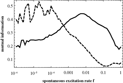
Figure 4. Same as Figure 3
B, but for N = 1024. The full curve shows the mutual information obtained from the similarity matrix C(f) and the matrix T; the dashed curve is the mutual information for C(f) and D.
Mean-Field Model
Following the lines of Graham and Matthai (2003) and Müller-Linow et al. (2006)
we formulate a mean-field description of the three-state excitable dynamics introduced in Section ‘Materials and Methods’. As we are interested in the rate of simultaneous excitations of two nodes, we include pair correlations in this model.
Denoting pα(t) the density of nodes in state α = e,r,s and qα,β(t) the probability that a pair of nodes is in state (α,β) at time t [obviously  and
and  ], mean-field evolution equations write:
and ], mean-field evolution equations write:
We can first make use of the mean-field description by discussing the average excitation density, which has been in the focus in Müller-Linow et al. (2006)
, as a function of the connectivity c (i.e., the number of links divided by the number N(N − 1)/2 of possible links). Figure 5
shows the excitation density pe obtained in the mean-field description, Eqs 3–7, as a function of the connectivity c. It is seen that this refined mean-field model (i.e., including pair correlations) nicely reproduces the increase of average excitation with connectivity.
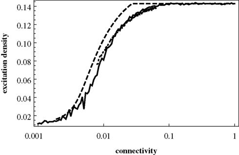
Figure 5. Mean-field excitation density pe as a function of the connectivity c. Dashed curve: prediction of pe obtained from the mean-field model including pair correlations; full curve: results from numerical simulations for Erdös–RÉnyi (ER) graphs; dotted curve: results from numerical simulations for Barabasi–Albert (BA) scalefree graphs; the general setup of the numerical simulations, including the model graph architectures, is the same as in Müller-Linow et al. (2006)
.
The joint excitation matrix (i.e., our prediction for the similarity matrix C) is then computed as the conditional correlation function Q(f, p) that two nodes are simultaneously excited knowing that they belong to the same topological class – shells around a central node, or modules. We performed the computation in two limiting regimes, first assuming that the dominant contribution comes from excitation of the central node (CN case) or from excitation from the middle node of even shortest paths (of length 2) within modules (TM case). In this computation, we can ignore the contribution of independent sources of excitation of the two nodes, and consider only the joint excitation initially caused by a unique remote firing event.
In the first case, the probability of excitation of the central node cannot be computed within the above mean-field approach due to the specific hub status of this node. Excitation of the hub comes from either the spontaneous firing of this node or the propagation of an excitation occurring at some node, with stationary probability pe, leading to:
where khub is the degree of the hub; it has to be multiplied by (1 − f) to ensure that the hub has not fired at the previous step and the excitation does not encounter a refractory hub. We compute the contribution  of shell n to Q(CN)(f)
of shell n to Q(CN)(f)
and get
where Sn is the number of nodes in shell n.
In the second case, all the shortest even paths between two nodes in the same module play the same role; the 2-step paths presumably give the dominant contribution. The network topology is involved through the average number ν of such paths, with roughly, ν = C(〈k〉 – 1) where C is the clustering coefficient. The analog quantity qee obtained for two nodes chosen at random has then to be subtracted. It then comes

Figure 6
shows Q(CN) and Q(TM) as a function of f. Comparing these curves with Figures 3 and 4
, it is obvious that we fail to account for any of the important features of the numerical results. In particular, Q(CN) does not decrease rapidly enough with f and Q(TM) does not show a peak at higher values of f. The switching of the two modes of organizing excitations on graphs is absent in this Figure.
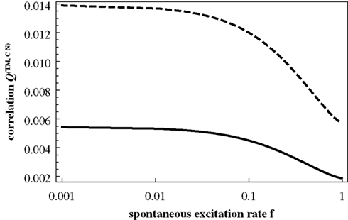
Figure 6. Q(CN) (from Eq. 10; dashed curve) and Q(TM) (from Eq. 11; full curve) as a function of f.
These two expressions Q(CN) and Q(TM) could be refined by introducing the precise number of loopless paths computed from reduced iterates of the adjacency matrix, but this does not change significantly the results.
Qualitatively, we can already say that the presence of large correlated events (dynamic heterogeneities in space and time) contradicts a mean-field view on the problem. We expect the approach to be fully valid only at large f, when the system reaches a stationary state (the behavior is then trivial, consisting in uncorrelated dynamics, with characteristic time scale 1 + 1/f + 1/p ≈ 2 + 1/p and no impact of the network topology).
The above equations account for pair correlations in the dynamic state (e.g.  ). This improves the plain mean-field approach and leads to a proper prediction of the average excitation density. But this model dramatically fails to reproduce the actual excitable dynamics and excitation patterns because it ignores large correlated spatio-temporal fluctuations, mainly transient and synchronized waves of excitation (‘avalanches’) spanning the effective network of susceptible nodes and shaped by network topology. Note that our approach does not account for pair correlations in the degree: Introducing the conditional degree distribution p(k′|k) and considering degree-dependent densities (averages over subsets of nodes with a given degree) in order to account for degree heterogeneity and correlation between neighbors (see e.g. Pastor-Satorras and Vespignani, 2004
), instead of the approximation using 〈k〉, would yield more complicated (analytically untractable) equations but still miss the essential dynamic correlation between neighboring nodes. It would not cure the failure of the mean-field approach to reproduce the correlation between excitation pattern and network topology. We rather turn to another formalism, explicitly describing the avalanches of excitation and how they reflect network topology.
). This improves the plain mean-field approach and leads to a proper prediction of the average excitation density. But this model dramatically fails to reproduce the actual excitable dynamics and excitation patterns because it ignores large correlated spatio-temporal fluctuations, mainly transient and synchronized waves of excitation (‘avalanches’) spanning the effective network of susceptible nodes and shaped by network topology. Note that our approach does not account for pair correlations in the degree: Introducing the conditional degree distribution p(k′|k) and considering degree-dependent densities (averages over subsets of nodes with a given degree) in order to account for degree heterogeneity and correlation between neighbors (see e.g. Pastor-Satorras and Vespignani, 2004
), instead of the approximation using 〈k〉, would yield more complicated (analytically untractable) equations but still miss the essential dynamic correlation between neighboring nodes. It would not cure the failure of the mean-field approach to reproduce the correlation between excitation pattern and network topology. We rather turn to another formalism, explicitly describing the avalanches of excitation and how they reflect network topology.Avalanche Model
The challenge is to combine a mean-field description of the dynamics with a suitable representation of topology in order to identify the typical effective network accessible to the dynamics as a function of the parameters f and p and the architecture of the network itself. This is the key idea proposed here for understanding the distribution of excitations as pattern on the graph. For random graphs (Erdös–Renyi graphs) the fluctuations in pe are distributed randomly across the graph. As soon as we provide a topological feature the fluctuations can exploit, these fluctuations lock onto the topological features. This is clearly seen when looking at the correlation between the above topological matrices T and D and the matrix C of simultaneous node excitations (Figure 3
).
We thus propose to understand the distribution of excitations as avalanches on the accessible parts of the network. A competition between p and f regulates the size of the effective networks and therefore the avalanche size and, more importantly, the topological features available to the dynamics. Avalanches have been discussed on abstract graphs (Lee et al., 2004
) and, in the context of self-organized criticality, in neural networks (see, e.g. Levina et al., 2007b
). While we are not discussing self-organized criticality here, we nevertheless employ the formal concept of avalanches as groups of excitation events correlated by the graph’s topology. In particular when the graph has a very heterogeneous degree distribution (and, more specifically, contains hubs) an avalanche of excitations propagating in the graph can be regarded as a two-step process: (1) the transportation of the excitation to the seed of the real avalanche, (2) the (amplified) spreading of the avalanche from the seed towards the accessible part of the graph.
Step (1), reminiscent of the coalescent view on a tree, is accounted for by considering the gathering of excitations at the seed i of an avalanche, yielding a factor equal to the degree ki of the seed. Step (2), close to the viewpoint adopted in branching processes, is accounted for by considering nested shells around the avalanche seed. To delineate the seed nodes, we might compute for each node i the multiplicative factor μi = k(i)S2(i): the probability that a node is a seed is identified with the weight  The density of susceptible nodes in shell n around i is computed in a mean-field approximation as:
The density of susceptible nodes in shell n around i is computed in a mean-field approximation as:
and the number of nodes in shell n is  where the matrices B(n) are computed recursively as B(0) = Id, B(1) = A,
  where H is the Heaviside function. The overall excitation amplification factor at node i is thus:
where the matrices B(n) are computed recursively as B(0) = Id, B(1) = A, where H is the Heaviside function. The overall excitation amplification factor at node i is thus:
The largest integer n for which  is appreciable gives the depth di(p, f) of an avalanche initiated at node i. The correlation (as regards their joint excitation) between two nodes j and l is finally given by:
is appreciable gives the depth di(p, f) of an avalanche initiated at node i. The correlation (as regards their joint excitation) between two nodes j and l is finally given by:
and the average size of an avalanche can be computed as:
Avalanches size and duration reveal the effective connectivity, while their location and frequency depend on f and the actual connectivity.
The idea of an effective graph is relevant only if recovery time is smaller than spontaneous firing period, namely p >> f. Also, speaking of avalanches makes sense only at low and moderate f (typically 1/f > 3): observing distinct avalanches (well-separated in space and time) requires slow driving: f << 1, a threshold dynamics (here all-or-none spontaneous excitation with probability f), and a rapid relaxation (diameter D << 1/f).
The distribution of weighting factors μi/Σq μq depends strongly on the detailed topological features of the graph. Essentially, the weighting factor μi/Σq μq gives the probability that a node i can trigger an avalanche of excitations. The actual size of the avalanche will then be determined by the effective (i.e. accessible) network of susceptible elements.
Figure 7
shows the correlation between the predicted similarity matrix Q and the matrices T and D derived from topology, together with the corresponding curves from Figure 3
B. The overall features of the numerical findings (red curves) are explained by the predictions (black curves), in particular the dominance of the hub distance captured in D at low f over the modules accounted for in T, the decrease of the correlation with D as a function of f and the increase of the correlation with T at high f.
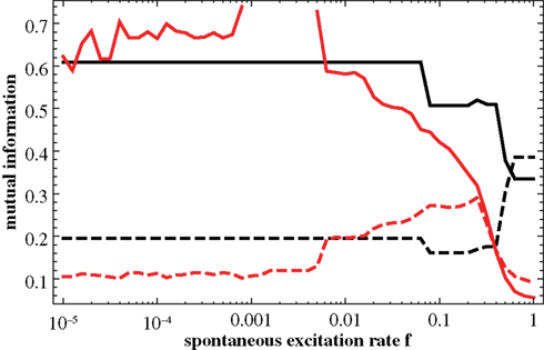
Figure 7. Mutual information as a function of f, measuring the correlation of the predicted similarity matrix Q with modularity (matrix T; black; full) and with distance to the central node (matrix D; black; dashed), compared to similar correlation measure between the simulated similarity matrix C and matrices T and D (red; respectively full and dashed); in all cases the 64-node hierarchical graph has been used.
When computing the matrix elements Qij giving the probability of the two nodes i and j being simultaneously excited, we assume that even for small f the observation time is long enough for the potential joint excitations of the two nodes to really unfold. Alternatively, we could have required some spontaneous excitation to have taken place (by inserting an additional factor of f). In the results from the numerical simulations we often observe a decrease of the correlation between the similarity matrix and topological matrices when going to small values of f. The above argument clearly identifies this behavior as a consequence of the finite simulation time. To support this interpretation we performed a longer simulation run for small f and found a systematic increase of the mutual information with simulation time, thus reducing the discrepancies between the numerical and analytical curves.
The results from Figure 7
have been obtained for the 64-node hierarchical graph. Figure 8
shows the corresponding results for the larger graph, N = 256. The lower two plots in Figure 8
compare these predictions with the relevant segments of the numerical curves (dashed) from Figure 4
. Again, the predictions clearly reproduce the increase of the one and the decrease of the other curve. In order to further assess, whether the predicted similarity matrices reproduce the actual distribution features of excitations on the graph, we compute the matrices Q(f) also for a scalefree graph (for which a dominance of a central-node type organization of excitations throughout a large regime of f is known from Müller-Linow et al. (2008) and for a modular, non-hierarchical graph (for which a dominance of the module-based organization of excitations has been observed across a broad range in f). Figure 9
summarizes these results. The predicted similarity matrices reproduce the numerical finding that on a scalefree graph (left) the central node-based pattern dominates and on a modular graph (right) the module-based pattern dominates across essentially the whole range of f.
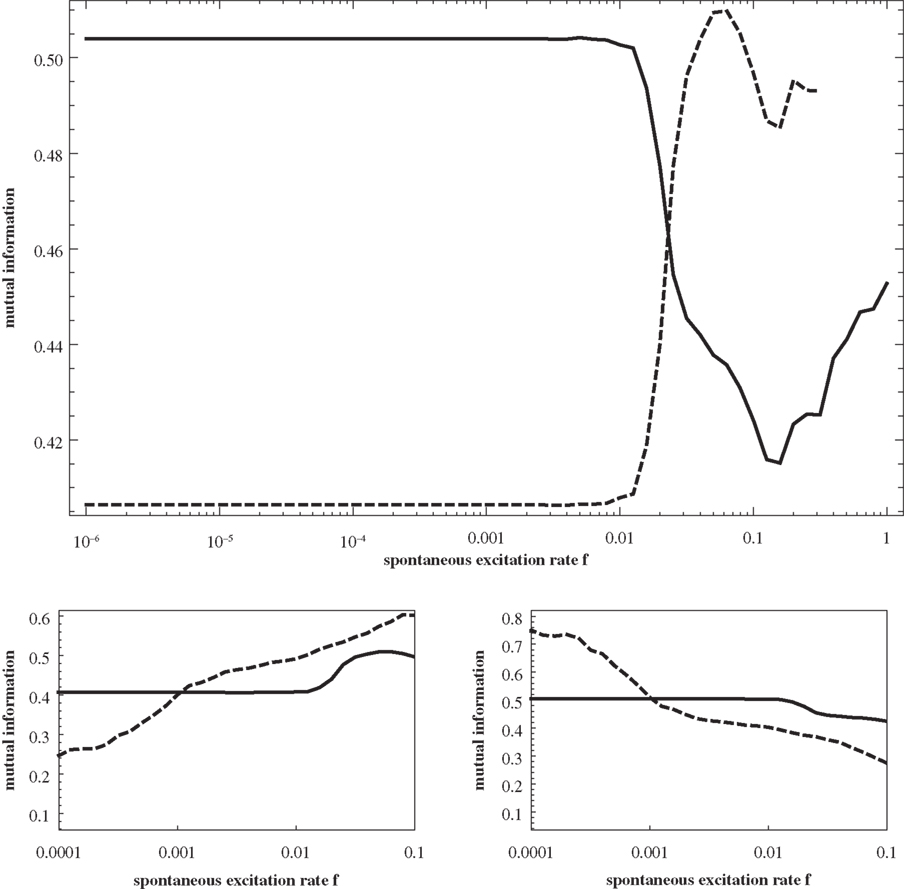
Figure 8. Upper figure: Mutual information as a function of f, measuring the correlation of the predicted similarity matrix Qij with modularity (matrix T; dashed curve) and with distance to the central node (matrix D; full curve). Compared to Figure 7
(N = 64) the graph size is now N = 256. The lower two figures compare each of these curves (left-hand side: modularity; right-hand side: central node; full curve: prediction; dashed curve: result from numerical simulation).
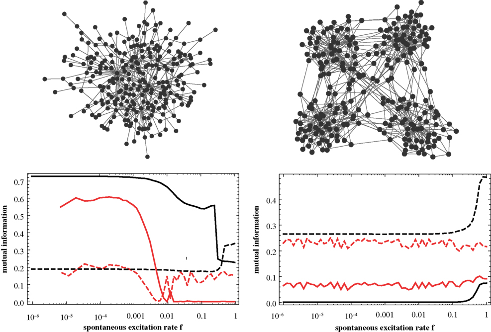
Figure 9. Top row: scalefree (BA) graph (left) and modular graph (right), each consisting of 256 nodes. Bottom row: For each of the graphs, mutual information as a function of f, measuring the correlation of the predicted similarity matrix Qij with modularity (matrix T; dashed curve) and with distance to the central node (matrix D; full curve). In both cases, numerical results are shown as well (red curves) based on a single 5000 time step simulation of the system on the graphs shown in the top row. In the case of the numerical result for the scalefree graph, two additional points should be noted: (1) as in Müller-Linow et al. (2008)
due to the high connectivity, the dynamics are re-scaled by requiring a certain percentage of neighbors (20%) to be active in order to activate a node; (2) at such small size, the population of scalefree graphs is very heterogeneous and therefore the curve can only be seen as a single-graph representative.
The systematic contribution to the correlations between topology and dynamics we observed comes from synchronized nodes. The amplification factor M(i) given above regulates the amount of simultaneously excited nodes in a particular topological class (a ring around the hub or a module) and therefore the strength of the synchronous signal.
For a given topological class an optimal duration T* of an avalanche as a function of f and p can be computed as the solution to T*mfR(p, f, T*) = 1 with  (effective recovery rate, defined as the probability that a site excited at time t = 0 has recovered and not yet experienced a spontaneous excitation at time T + 1). This time T*(p, f) is expected to be the relevant ‘recovery time’, separating two avalanches. Comparing 1/f (i.e., the typical time scale available to an avalanche) with T* should give the expected peak in the correlation of the similarity matrix to this topological class.
(effective recovery rate, defined as the probability that a site excited at time t = 0 has recovered and not yet experienced a spontaneous excitation at time T + 1). This time T*(p, f) is expected to be the relevant ‘recovery time’, separating two avalanches. Comparing 1/f (i.e., the typical time scale available to an avalanche) with T* should give the expected peak in the correlation of the similarity matrix to this topological class.Our main finding is that we can explain the qualitative feature of the switching from central node dominated to a module dominated organization of the dynamics, as the rate of spontaneous excitation f is increased.
It should be pointed out that this switching is not a dynamic phase transition. In particular, we do not observe the switching to become sharper with increasing graph size.
The main motivation for our use of avalanches is that excitations spread on the effective network (consisting of the nodes in the susceptible state at a given moment in time), whose topological properties depend on f and in turn on the previous history of the dynamics.
A random excitation will trigger a certain cascade of joint excitations of other nodes. The sizes of these contributions to the similarity matrix (and the nodes involved in these contributions) depend strongly on the effective network. At large f, random excitations follow so rapidly one after another that only few nodes in the graph are susceptible, leading to only few and small-scale contributions to the similarity matrix. At small f, on the other hand, the graph has enough time to recover between consecutive random excitations, allowing each random excitation to essentially trigger a whole avalanche of joint excitations.
In Figure 10
the average shortest path length of the effective networks as a function of f. According to our avalanche concept, we believe that this decrease of the average path length with f, which is clearly discernible in Figure 10
, is the main driving force of the switching behavior.
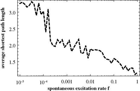
Figure 10. Average shortest path length for effective networks formed by susceptible elements at each time step of the numerical simulation of the dynamics. In order to compute this curve for each value of f we used a 10,000 time step simulation of the dynamics on the 256-node hierarchical graph, for each effective network averaged over the shortest paths between all nodes and, finally, averaged over the effective networks from 1000 time steps.
We are mainly interested in understanding the global interplay and network effect, not only the local consequences of a node or motif topological specificity. Accordingly, we analyzed the relation between topology and dynamics with methods from spatiotemporal pattern formation. When the carrier space is no longer a regular lattice, it becomes relevant to investigate the origin of the pattern and the shaping of the patterns by network topology. This can be achieved by studying correlations between topological properties and properties of the dynamics. The results reflect the exploitation of certain topological features by dynamics. In particular, by computing the mutual information between the respective matrices, we show the f-dependence of the correlation between topology and dynamics and re-discover the dependence as discussed previously with other means (Müller-Linow et al., 2008
).
Here we have been able to understand the dominant features of these patterns from Müller-Linow et al. (2008)
analytically using a combination of a mean-field approach and avalanche viewpoint: on a hierarchical graph, the core feature is the switching from a ‘central-node’ to a ‘topological-module’ mode of organization of simultaneous excitations as a function of f; on scalefree and modular graphs, it is the dominance of one of the modes across the whole range of f.
We have also shown that the mean-field model reasonably well explains the increase of the average excitation density as a function of connectivity, which was reported in Müller-Linow et al. (2006)
.
Due to its very principles and associated approximations, the mean-field model can describe average properties of the excitations, but not the interplay between topology and dynamics (i.e., how topological features regulate the distribution patterns of excitations on the graph). In fact, the validity of the mean-field approach depends on the investigated feature. For instance, when looking at the curve of average excitation as a function of connectivity, only a very small dependence on graph topology is seen (Müller-Linow et al., 2006
), and the mean-field description is here in good agreement with the numerical data. But it fails to account for the two regimes of correlation between topology and dynamics observed as a function of f, whose origin is unraveled and quantitatively captured in our avalanche description.
Several important steps are left for future work: In order to develop a global picture of this interplay between topology and dynamics one needs to study the topological properties of the effective networks and, therefore, the size distribution of the avalanches as a function of topology and system parameters. As discussed at the end of the results section, our current formalism already leads to some predictions for the time scales relevant for avalanches of excitations, as well as for the avalanche size and duration distributions. An extension of this formalism may help us link the observations from this simple model of excitations to the formalisms discussed in Levina et al. (2007a
,b
).
We also believe that the distribution of weighting factors μi and amplification factors M(i) may provide interesting characterizations of a network for dynamical purposes. This certainly needs further exploration.
The authors declare that the research was conducted in the absence of any commercial or financial relationships that could be construed as a potential conflict of interest.
We are indebted to Mark Müller-Linow (Darmstadt, Germany) for providing the first set of numerical simulations we here compare our analytical predictions with. We wish to thank Claus Hilgetag (Bremen, Germany) for fruitful discussions on this topic. M.H. acknowledges generous support from the IHÉS guest program for the purposes of this work; A.L. has been a visitor of the ICTS program at Jacobs University during the completion of this work. Publication of this work has been supported by the Agence Nationale de la Recherche (ANR 05-NANO-062-03 ‘CHROMATOPINCES’).