1
Honda Research Institute Europe GmbH, Offenbach, Germany
2
Bernstein Center for Computational Neuroscience, Albert-Ludwig University, Freiburg, Germany
3
Laboratory for Computational Neuroscience, Swiss Federal Institute of Technology, EPFL, Lausanne, Switzerland
4
Theoretical Neuroscience Group, RIKEN Brain Science Institute, Wako City, Japan
5
Brain and Neural Systems Team, Computational Science Research Program, RIKEN, Wako City, Japan
The neural simulation tool NEST (
http://www.nest-initiative.org
) is a simulator for heterogeneous networks of point neurons or neurons with a small number of compartments. It aims at simulations of large neural systems with more than 104 neurons and 107 to 109 synapses. NEST is implemented in C++ and can be used on a large range of architectures from single-core laptops over multi-core desktop computers to super-computers with thousands of processor cores. Python (http://www.python.org
) is a modern programming language that has recently received considerable attention in Computational Neuroscience. Python is easy to learn and has many extension modules for scientific computing (e.g. http://www.scipy.org
). In this contribution we describe PyNEST, the new user interface to NEST. PyNEST combines NEST’s efficient simulation kernel with the simplicity and flexibility of Python. Compared to NEST’s native simulation language SLI, PyNEST makes it easier to set up simulations, generate stimuli, and analyze simulation results. We describe how PyNEST connects NEST and Python and how it is implemented. With a number of examples, we illustrate how it is used.
The first user interface for NEST (Gewaltig and Diesmann, 2007
; Plesser et al., 2007
) was the simulation language SLI, a stack-based language derived from PostScript (Adobe Systems Inc., 1999
). However, programming in SLI turned out to be difficult to learn and users asked for a more convenient programming language for NEST.
When we decided to use Python as the new simulation language, it was almost unknown in Computational Neuroscience. In fact, Matlab (MathWorks, 2002
) was far more common, both for simulations and for analysis. Other simulators, like e.g. CSIM (Natschläger, 2003
), already used Matlab as their interface language. Thus, Matlab would have been a natural choice for NEST as well.
Python has a number of advantages over commercial software like Matlab and other free scripting languages like Tcl/Tk (Ousterhout, 1994
). First, Python is installed by default on all Linux and Mac-OS based computers. Second, Python is stable, portable, and supported by a large and active developer community, and has a long history in scientific fields outside the neurosciences (Dubois, 2007
). Third, Python is a powerful interactive programming language with a surprisingly concise and readable syntax. It supports many programming paradigms such as object-oriented and functional programming. Through packages like NumPy (
http://www.numpy.org
) and SciPy (http://www.scipy.org
), Python supports scientific computing and visualization à la Matlab. Finally, a number of neuroscience laboratories meanwhile use Python for simulation and analysis, which further supports our choice.Python is powerful at steering other applications and provides a well documented interface (API) to link applications to Python (van Rossum, 2008
). To do so, it is common to map the application’s functions and data structures to Python classes and functions. This approach has the advantage that the coupling between the application and Python is as tight as possible. But there is also a drawback: Whenever a new feature is implemented in the application, the interface to Python must be changed as well.
On many high-performance computers Python is not available and we have to preserve NEST’s native simulation language SLI. In order to avoid two different interfaces, one to Python and one to SLI, we decided to deviate from the standard way of coupling applications to Python. Rather than using NEST’s classes, we use NEST’s simulation language as the interface: Python sends data and SLI commands to NEST and NEST responds with Python data structures.
Exchanging data between Python and NEST is easy since all important data types in NEST have equivalents in Python. Executing NEST commands from Python is also straightforward: Python only needs to send a string with commands to NEST, and NEST will execute them. With this approach, we only need to maintain one binary interface to the simulation kernel instead of two: Each new feature of the simulation kernel only needs to be mapped to SLI and immediately becomes accessible in PyNEST without changing its binary interface. This generic interpreter interface allows us to program PyNEST’s high-level API in Python. This is an advantage, because programming in Python is more productive than programming in C++ (Prechelt, 2000
). Python is also more expressive: A given number of lines of Python code achieve much more than the same number of lines in C++ (McConnell, 2004
).
NEST users benefit from the increased productivity. They can now take advantage of the large number of extension modules for Python. NumPy is the Python interface to the BLAS libraries, the same libraries which power Matlab. Matplotlib (
http://matplotlib.sourceforge.net
) provides many routines to plot scientific data in publication quality. Many other packages exist to analyze and visualize data. Thus, PyNEST allows users to combine simulation, data analysis, and visualization in a single programming language.In the Section “Using PyNEST”, we introduce the basic modeling concepts of NEST. With a number of PyNEST code examples, we illustrate how simulations are defined and how the results are analyzed and plotted. In the Section “The Interface Between Python and NEST”, we describe in detail how we bind NEST to the Python interpreter. In the Section “Discussion”, we discuss our implementation and analyze its performance. The complete API reference for PyNEST is contained in Appendix A. In Appendix B we illustrate advanced PyNEST features, using a large scale model.
A neural network in NEST consists of two basic element types: Nodes and connections. Nodes are either neurons, devices or subnetworks. Devices are used to stimulate neurons or to record from them. Nodes can be arranged in subnetworks to build hierarchical networks like layers, columns, and areas. After starting NEST, there is one empty subnetwork, the so-called root node. New nodes are created with the command
Create(), which takes the model name and optionally the number of nodes as arguments and returns a list of handles to the new nodes. These handles are integer numbers, called ids. Most PyNEST functions expect or return a list of ids (see Appendix A). Thus it is easy to apply functions to large sets of nodes with a single function call.Nodes are connected using
Connect(). Connections have a configurable delay and weight. The weight can be static or dynamic, as for example in the case of spike timing dependent plasticity (STDP; Morrison et al., 2008
). Different types of nodes and connections have different parameters and state variables. To avoid the problem of fat interfaces (Stroustrup, 1997
), we use dictionaries with the functions GetStatus() and SetStatus() for the inspection and manipulation of an element’s configuration. The properties of the simulation kernel are controlled through the commands GetKernelStatus() and SetKernelStatus(). PyNEST contains the submodules raster_plot and voltage_trace to visualize spike activity and membrane potential traces. They use Matplotlib internally and are good templates for new visualization functions. However, it is not our intention to develop PyNEST into a toolbox for the analysis of neuroscience data; we follow the modularity concept of Python and leave this task to others (e.g. NeuroTools, http://www.neuralensemble.org/NeuroTools
).Example
We illustrate the key features of PyNEST with a simulation of a neuron receiving input from an excitatory and an inhibitory population of neurons (modified from Gewaltig and Diesmann, 2007
). Each presynaptic population is modeled by a Poisson generator, which generates a unique Poisson spike train for each target. The simulation adjusts the firing rate of the inhibitory input population such that the neurons of the excitatory population and the target neuron fire at the same rate.
First, we import all necessary modules for simulation, analysis and plotting.
Third, the nodes are created using
Create(). Its arguments are the name of the neuron or device model and optionally the number of nodes to create. If the number is not specified, a single node is created. Create() returns a list of ids for the new nodes, which we store in variables for later reference.
Fourth, the excitatory Poisson generator (
noise[0]) and the voltmeter are configured using SetStatus(), which expects a list of node handles and a list of parameter dictionaries. The rate of the inhibitory Poisson generator is set in line 32. For the neuron and the spike detector we use the default parameters.
Fifth, the neuron is connected to the spike detector and the voltmeter, as are the two Poisson generators to the neuron:
The command
Connect() has different variants. Plain Connect() (line 26 and 27) just takes the handles of pre- and postsynaptic nodes and uses the default values for weight and delay. ConvergentConnect() (line 28) takes four arguments: A list of presynaptic nodes, a list of postsynaptic nodes, and lists of weights and delays. It connects all presynaptic nodes to each postsynaptic node. All variants of the Connect() command reflect the direction of signal flow in the simulation kernel rather than the physical process of inserting an electrode into a neuron. For example, neurons send their spikes to a spike detector, thus the neuron is the first argument to Connect() in line 26. By contrast, a voltmeter polls the membrane potential of a neuron in regular intervals, thus the voltmeter is the first argument of Connect() in line 27. The documentation of each model explains the types of events it can send and receive.To determine the optimal rate of the neurons in the inhibitory population, the network is simulated several times for different values of the inhibitory rate while measuring the rate of the target neuron. This is done until the rate of the inhibitory neurons is determined up to a given relative precision (
prec), such that the target neuron fires at the same rate as the neurons in the excitatory population. The algorithm is implemented in two steps:First, the function
output_rate() is defined to measure the firing rate of the target neuron for a given rate of the inhibitory neurons.
The function takes the firing rate of the inhibitory neurons as an argument. It scales the rate with the size of the inhibitory population (line 31) and configures the inhibitory Poisson generator (
noise[1]) accordingly (line 32). In line 33, the spike-counter of the spike detector is reset to zero. Line 34 simulates the network using Simulate(), which takes the desired simulation time in milliseconds and advances the network state by this amount of time. During the simulation, the spike detector counts the spikes of the target neuron and the total number is read out at the end of the simulation period (line 35). The return value of output_rate() is an estimate of the firing rate of the target neuron in Hz.Second, we determine the optimal firing rate of the neurons of the inhibitory population using the bisection method.

The SciPy function
bisect() takes four arguments: First a function whose zero crossing is to be determined. Here, the firing rate of the target neuron should equal the firing rate of the neurons of the excitatory population. Thus we define an anonymous function (using lambda) that returns the difference between the actual rate of the target neuron and the rate of the excitatory Poisson generator, given a rate for the inhibitory neurons. The next two arguments are the lower and upper bound of the interval in which to search for the zero crossing. The fourth argument of bisect() is the desired relative precision of the zero crossing.Finally, we plot the target neuron’s membrane potential as a function of time.

A transcript of the simulation session and the resulting plot are shown in Figure 1
.
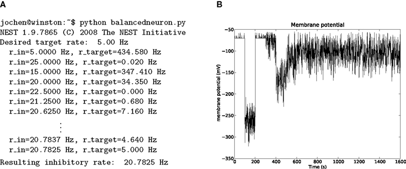
Figure 1. Results of the example simulation. (A) The transcript of the simulation session shows the intermediate results of
r_target as bisect() searches for the optimal rate. (B) The membrane potential of the target neuron as a function of time. Repeated adjustment of the spike rate of the inhibitory population by bisect() results in a convergence of the mean membrane potential to −112 mV, corresponding to an output spike rate of 5.0 Hz.PyNEST on Multi-Core Processors and Clusters
NEST has built-in support for parallel and distributed computing (Morrison et al., 2005
; Plesser et al., 2007
): On multi-core processors, NEST uses POSIX threads (Lewis and Berg, 1997
), on computer clusters, NEST uses the Message Passing Interface (MPI; Message Passing Interface Forum, 1994
). Nodes and connections are assigned automatically to threads and processes, i.e. the same script can be executed single-threaded, multi-threaded, distributed over multiple processes, or using a combination of both methods. This naturally carries over to PyNEST: To use multiple threads for the simulation, the desired number has to be set prior to the creation of nodes and connections. Note that the network setup is carried out by a single thread, as only a single instance of the Python interpreter exists in each process. Only the simulation takes advantage of multiple threads. Distributed simulations can be run via the
mpirun command of the respective MPI implementation. Where, for SLI, one would execute mpirun -np n nest simulation.sli to distribute a simulation onto n processes, one has to call mpirun -np n python simulation.py to get the same result with PyNEST. In the distributed case, n Python interpreters run in parallel and execute the same simulation script. This means that both network setup and simulation are parallelized. With third-party tools like IPython (http://ipython.scipy.org
) or MPI for Python (http://mpi4py.scipy.org
), it is possible to use PyNEST interactively even in distributed scenarios. For a more elaborate documentation of parallel and distributed simulations with NEST, see the NEST user manual (http://www.nest-initiative.org
).NEST’s built-in simulation language (SLI) is a stack-based language in which functions expect their arguments on an operand stack to which they also return their results. This means that in every expression, the arguments must be entered before the command that uses them (reverse polish notation). For many new users, SLI is difficult to learn and hard to read. This is especially true for math: The simple expression α = t · e−t/τ has to be written as /
alpha t t neg tau div exp mul def in SLI. But SLI is also a high-level language where functions can be assembled at run time, stored in variables and passed as arguments to other functions (functional programming; Finkel, 1996
). Powerful indexing operators like Part and functional operators like Map, together with data types like heterogeneous arrays and dictionaries, allow a compact and expressive formulation of algorithms.Stack-based languages are often used as intermediate languages in compilers and interpreters (Aho et al., 1988
). This inspired us to couple NEST and Python using SLI as an intermediate language.
The PyNEST Low-Level Interface
The low-level API of PyNEST is implemented in C/C++ using the Python C-API (van Rossum, 2008
). It exposes only three functions to Python, and has private routines for converting between SLI data types and their Python equivalents. The exposed functions are:
1.
2.
3.
sli_push(py_object), which converts the Python object py_object to the corresponding SLI data type and pushes it onto SLI’s operand stack.2.
sli_pop(), which removes the top element from SLI’s operand stack and returns it as a Python object.3.
sli_run(slicommand), which uses NEST’s simulation language interpreter to execute the string slicommand. If the command requires arguments, they have to be present on SLI’s operand stack or must be part of slicommand. After the command is executed, its return values will be on the interpreter’s operand stack.Since these functions provide full access to the simulation language interpreter, we can now control NEST’s simulation kernel without explicit Python bindings for all NEST functions. This interface also provides a natural way to execute legacy SLI code from within a PyNEST script by just using the command
sli_run(“(legacy.sli) run”). However, it does not provide any benefits over plain SLI from a syntactic point of view: All simulation specific code still has to be written in SLI. This problem is solved by a set of high-level functions.The PyNEST High-Level Interface
To allow the researcher to define, run and evaluate NEST simulations using only Python, PyNEST offers convenient wrappers for the most important functions of NEST. These wrappers are implemented on top of the low-level API and execute appropriate SLI expressions. Thus, at the level of PyNEST, SLI is invisible to the user. Each high-level function consists essentially of three parts:
1. The arguments of the function are put on SLI’s operand stack.
2. One or more SLI commands are executed to perform the desired action in NEST.
3. The results (if any) are fetched from the operand stack and returned as Python objects.
2. One or more SLI commands are executed to perform the desired action in NEST.
3. The results (if any) are fetched from the operand stack and returned as Python objects.
A concrete example of the procedure is given in the following listing, which shows the implementation of
Create():
In line 2, we first transfer the model name to NEST. Model names in NEST have to be of type literal, a special symbol type that is not available in Python. Because of this, we cannot use
sli_push() for the data transfer, but have to use sli_run(), which executes a given command string instead of just pushing it onto SLI’s stack. The command string consists of a slash followed by the model name, which is interpreded as a literal by SLI. Line 3 uses sli_push() to transmit the number of nodes (n) to SLI. The nodes are then created by CreateMany in line 4, which expects the model name and number of nodes on SLI’s operand stack and puts the id of the last created node back onto the stack. The id is retrieved in line 5 via sli_pop(). To be consistent with the convention that all PyNEST functions work with lists of nodes, we build a list of all created nodes’ ids, which is returned in line 6.A sequence diagram of the interaction between the different software layers of PyNEST is shown in Figure 2
for a call to the
Create() function.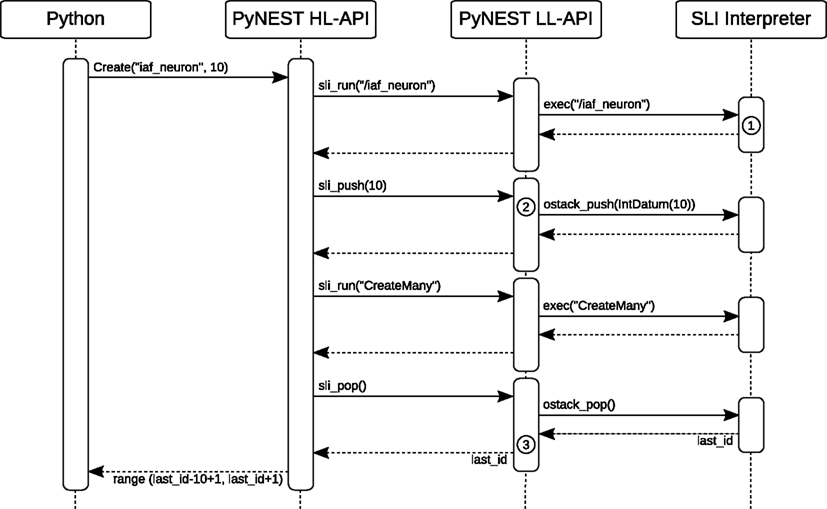
Figure 2. Sequence diagram showing the interaction between Python and SLI. A call to the PyNEST high-level function  ). Next, it pushes the number of nodes (10) to SLI using
  ) and pushes it onto SLI’s operand stack. Next, it executes appropriate SLI code to create the nodes of type
  ). The result of the operation in SLI (the id of the last node created) is used to create a list with the ids of all new nodes, which is returned to Python.
Create() first transmits the model name to SLI using sli_run(). It is converted to the SLI type
literal by the interpreter (). Next, it pushes the number of nodes (10) to SLI using sli_push(). The PyNEST low-level API converts the argument to a SLI datum () and pushes it onto SLI’s operand stack. Next, it executes appropriate SLI code to create the nodes of type iaf_neuron in the simulation kernel. Finally it retrieves the results of the NEST operations using sli_pop(), which converts the data back to a Python object (). The result of the operation in SLI (the id of the last node created) is used to create a list with the ids of all new nodes, which is returned to Python.Data Conversion
The data conversion between Python and SLI exploits the fact that most data types in SLI have an equivalent type in Python. The function in Figure 2
).
sli_push() calls PyObjectToDatum() to convert a Python object py_object to the corresponding SLI data type (see in Figure 2
). PyObjectToDatum() determines the type of py_object in a cascade of type checks (e.g. PyInt_Check(), PyString_Check(), PyFloatCheck()) as described by van Rossum (2008)
. If a type check succeeds, the Python object is used to create a new SLI Datum of the respective type. PyObjectToDatum() is called recursively on the elements of lists and dictionaries. The listing below shows how this technique is used for the conversion of the Python type float and for NumPy arrays of doubles:
To convert a SLI data type to the corresponding Python type, we can avoid the cascade of type checks, since all SLI data types are derived from a common base class, called
Datum. The C++ textbook solution would add a pure virtual conversion function convert() to the class Datum. Each derived class (e.g. DoubleDatum,DoubleVectorDatum) then overloads this function to implement its own conversion to the corresponding Python type. This approach is shown for the SLI type DoubleDatum in the following listing. The function get() is implemented in each Datum and returns its data member.
However, this solution would make SLI’s type hierarchy (and thus NEST) depend on Python. To keep NEST independent of Python, we split the implementation in two parts: The first is Python-unspecific and resides in the NEST source code (Figure 3
, left rectangle), the second is Python-specific and defined in the PyNEST source code (Figure 3
, right rectangle).
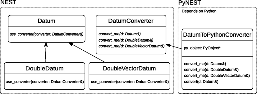
Figure 3. Class diagram for the acyclic visitor pattern used to convert SLI types to Python types. The left rectangle contains classes belonging to NEST, the right rectangle contains classes that are part of PyNEST. All SLI data types are derived from the base class
Datum and inherit its function use_converter(). The class DatumConverter is the base class of DatumToPythonConverter. The actual data conversion is carried out in one of DatumToPythonConverter’s convert_me() functions. Virtual functions are typeset in italics.We move the Python-specific conversion code from
convert() to a new function convert_me(), which is then called by the interface function use_converter(). This function is now independent of Python:
The function
use_converter() is defined in the base class Datum and inherited by all derived classes. It calls the convert_me() function of converter that matches the type of the derived Datum. NEST’s class DatumConverter is an abstract class that defines a pure virtual function convert_me(T&) for each SLI type T:
The Python-specific part of the conversion is encapsulated in the class
DatumToPythonConverter, which derives from DatumConverter and implements the convert_me() functions to actually convert the SLI types to Python objects. DatumToPythonConverter::convert_me() takes a reference to the Datum as an argument and is overloaded for each SLI type. It stores the result of the conversion in the class variable py_object. An example for the conversion of DoubleDatum is given in the following listing:
DatumToPythonConverter also provides the function convert(), which converts a given Datum d to a Python object by calling d.use_converter() with itself as an argument. It is used in the implementation of sli_pop() (see in Figure 2
). After the call to use_converter(), the result of the conversion is available in the member variable py_object, and is returned to the caller:
In the Computer Science literature, this method of decoupling different parts of program code is called the acyclic visitor pattern (Martin et al., 1998
). Our implementation is based on Alexandrescu (2001)
.
As an example, the diagram in Figure 4
illustrates the sequence of events in
sli_pop(): First, sli_pop() retrieves a SLI Datum d from the operand stack (not shown). Second, it creates an instance of DatumToPythonConverter and calls its convert() function, which then passes itself as visitor to the use_converter() function of d. Datum::use_converter() calls the DatumToPythonConverter’s convert_me() function that matches the type of d. The function convert_me() then creates a new Python object from the data in d and stores it in the DatumToPythonConverter’s member variable py_object, which is returned to sli_pop().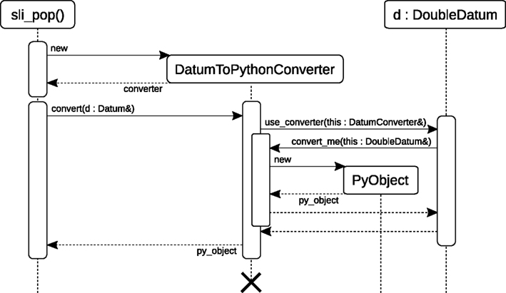
Figure 4. Sequence diagram of the acyclic visitor pattern for data conversion from SLI to Python. For the conversion of a SLI datum
d, sli_pop() creates an instance of DatumToPythonConverter. It then calls the DatumToPythonConverter’s convert() function, which passes itself as a visitor to the use_converter() function of d. Datum::use_converter() calls the DatumToPythonConverter’s convert_me() function that matches d’s type. convert_me() creates a new Python object from the data contained in d. The new Python object is returned to sli_pop().To make PyNEST depend on NumPy only if it is available, we use conditional compilation based on the preprocessor macro
HAVE_NUMPY, which is determined during the configuration of PyNEST prior to compilation. For example, the following listing shows the implementation of the DatumToPythonConverter::convert_me() function to convert homogeneous arrays of doubles from SLI to Python. If NumPy is available during compilation, its homogeneous array type is used to store the data. Without NumPy, a Python list is used instead.
Error Handling
Error handling in NEST is implemented using C++ exceptions that are propagated up the calling hierarchy until a suitable error handler catches them. In this section, we describe how we extend this strategy to PyNEST.
PyNEST executes SLI code using
sli_run() as described in the Section “The PyNEST High-Level Interface”. However, the high-level API does not call sli_run() directly, but rather through the wrapper function catching_sr():
In line 2,
catching_sr() converts the command string cmd to a SLI procedure by adding braces. It then calls the SLI command runprotected (see listing below), which executes the procedure in a stopped context (PostScript; Adobe Systems Inc., 1999
). If an error occurs, stopped leaves the name of the failed command on the stack and returns true. In this case, runprotected extracts the name of the error from SLI’s error dictionary, converts it to a string, and puts it back on the operand stack, followed by false to indicate the error condition to the caller. Otherwise, true is put on the stack. In case of an error, catching_sr() uses both the name of the command and the error to raise a Python exception (NESTError), which can be handled by the user’s simulation code. The following listing shows the implementation of runprotected:
Forwarding the original NEST errors to Python has the advantage that PyNEST functions do not have to check their arguments, because the underlying NEST functions already do. This makes the code of the high-level API more readable, while at the same time, errors are raised as Python exceptions without requiring additional code. Moreover, this results in consistent error messages in NEST and PyNEST.
The previous sections describe the usage and implementation of PyNEST. Here we discuss consequences and limitations of the PyNEST implementation.
Performance
The use of PyNEST entails a certain computational overhead over pure SLI-operated NEST. This overhead can be split into two main components:
1. Call overhead because of using SLI over direct access to the NEST kernel.
2. Data exchange between Python and NEST.
2. Data exchange between Python and NEST.
For most real-world simulations, the first is negligible, since the number of additional function calls is small. In practice, most overhead is caused by the second component, which we can reduce by minimizing the number of data conversions. For an illustration of the technique, see the following two listings that both add up a sequence of numbers in SLI. The first creates the sequence of numbers in Python, pushes them to SLI one after the other and lets SLI add them. Executing it takes approx. 15 s on a laptop with an Intel Core Duo processor at 1.83 GHz.
The second version computes the same result, but instead of creating the sequence in Python, it is created in SLI:

Although Python loops are about twice as fast as SLI loops, this version takes only 0.6 s, because of the reduced number of data conversions and, to a minor extent, the repeated parsing of the command string and the larger number of function calls in the first version.
The above technique is used in the implementation of the PyNEST high-level API wherever possible. The same technique is also applied for other loop-like commands (e.g.
Map) that exist in both interpreters. However, it is important to note that the total run time of the simulation is often dominated by the actual creation and update of nodes and synapses, and by event delivery. These tasks take place inside of the optimized C++ code of NEST’s simulation kernel, hence the choice between SLI or Python has no impact on performance.Independence
One of the design decisions for PyNEST was to keep NEST independent of third-party software. This is important because NEST is used on architectures, where Python is not available or only available as a minimal installation. Moreover, since NEST is a long term project that has already seen several scripting languages and graphics libraries coming and going, we do not want to introduce a hard dependency on one or the other. The stand-alone version of NEST can be compiled without any third-party libraries. Likewise, the implementation of PyNEST does not depend on anything except Python itself. The use of NumPy is recommended, but optional. The binary part of the interface is written by hand and does not depend on interface generators like SWIG (
http://www.swig.org
) or third-party libraries like Boost.Python (http://www.boost.org
). In our opinion, this strategy is important for the long-term sustainability of our scientific software.Extensibility
NEST can never provide all models and functions needed by every researcher. Extensibility is hence important.
Due to the asymmetry of the PyNEST interface (see “Assymmetry of the Interface”), neuron models, devices and synapse models have to be implemented in C++, the language of the simulation kernel. However, new analysis functions and connection routines can be implemented in either Python, SLI or C++, depending on the performance required and the skills of the user. The implementation in Python is easy, but performance may be limited. However, this approach is safe, as the real functionality is performed by SLI code, which is often well tested. To improve the performance, the implementation can be translated to SLI. This requires knowledge of SLI in addition to Python. Migrating the function down to the C++ level yields the highest performance gain, but requires knowledge of C++ and the internals of the simulation kernel.
Since the user can choose between three languages, it is easy to extend PyNEST, while at the same time, it is possible to achieve high performance if necessary. The hierarchy of languages also provides abstraction layers, which make it possible to migrate the implementation of a function between the different languages, without affecting user code. The intermediate layer of SLI allows the decoupling of the development of the simulation kernel from the development of the PyNEST API. This is also helpful for developers of abstraction libraries like PyNN (Davison et al., 2008
), who only need limited knowledge of the simulation kernel.
Assymmetry of the Interface
Our implementation of PyNEST is asymmetric in that SLI code can be executed from Python, but NEST cannot respond, except for error handling and data exchange. Although this is sufficient to run NEST simulations from within a Python session, it could be beneficial to allow NEST to execute Python code: The user of PyNEST already knows the Python programming language, hence it might be easier to extend NEST in Python rather than to modify the C++ code of the simulation kernel. SciPy, NumPy and other packages provide well tested implementations of mathematical functions and numerical algorithms. Together with callback functions, these libraries would allow rapid prototyping of neuron and synapse models or to initialize parameters of neuron models or synapses according to complicated probability distributions: Python could be the middleware between NEST’s simulation kernel and the numerical package. Using online feedback from the simulation, callback functions could also control simulations. Moreover, with a symmetric interface and appropriate Python modules it would be easier to add graphical user interfaces to NEST, along with online display of observables, and experiment management.
Different implementations of the symmetric interface are possible: One option is to pass callback functions from Python to NEST. Another option is to further exploit the idea that the “language is the protocol”. In the same way as PyNEST generates SLI code, NEST would emit code for Python. Already Harrison and McLennan (1998)
mention this technique, and in experimental implementations it was used successfully to symmetrically couple NEST with Tcl/Tk (Diesmann and Gewaltig, 2002
), Mathematica, Matlab and IDL. The fact that none of these interfaces is still maintained confirms the conclusions of the Section “Independence”.
Language Considerations
At present, PyNEST maps NEST’s capabilities to Python. Further advances in the expressiveness of the language may be easier to achieve at the level of Python or above (e.g. PyNN; Davison et al., 2008
) without a counterpart in SLI. An example for this is the support of units for physical quantities as available in SBML (Hucka et al., 2002
) or Brian (Goodman and Brette, 2008
).
More generally, the development of simulation tools has not kept up with the increasing complexity of network models. As a consequence the reliable documentation of simulation studies is challenging and laboratories notoriously have difficulties in reproducing published results (Djurfeldt and Lansner, 2007
). One component of a solution is the ability to concisely formulate simulations in terms of the neuroscientific problem domain like connection topologies and probability distributions. At present little research has been carried out on the particular design of such a language (Davison et al., 2008
; Nordlie et al., 2008
), but a general purpose high-level language interface to the simulation engine is a first step towards this goal.
A. PyNEST API Reference
Models(mtype=“all”, sel=None): Return a list of all available models (nodes and synapses). Use mtype=“nodes” to only see node models, mtype=“synapses” to only see synapse models. sel can be a string, used to filter the result list and only return models containing it.GetDefaults(model): Return a dictionary with the default parameters of the given model, specified by a string.SetDefaults(model, params): Set the default parameters of the given model to the values specified in the params dictionary.GetStatus(model, keys=None): Return a dictionary with status information for the given model. If keys is given, a value is returned instead. keys may also be a list, in which case a list of values is returned.CopyModel(existing, new, params=None): Create a new model by copying an existing one. Default parameters can be given as params, or else are taken from existing.Create(model, n=1, params=None): Create n instances of type model in the current subnetwork. Parameters for the new nodes can be given as params (a single dictionary, or a list of dictionaries with size n). If omitted, the model’s defaults are used.GetStatus(nodes, keys=None): Return a list of parameter dictionaries for the given list of nodes. If keys is given, a list of values is returned instead. keys may also be a list, in which case the returned list contains lists of values.SetStatus(nodes, params, val=None): Set the parameters of the given nodes to params, which may be a single dictionary, or a list of dictionaries of the same size as nodes. If val is given, params has to be the name of a property, which is set to val on the nodes. val can be a single value, or a list of the same size as nodes.Connect(pre, post, params=None, delay=None, model=“static_synapse”): Make one-to-one connections of type model between the nodes in pre and the nodes in post. pre and post have to be lists of the same length. If params is given (as a dictionary or as a list of dictionaries with the same size as pre and post), they are used as parameters for the connections. If params is given as a single float, or as a list of floats of the same size as pre and post, it is interpreted as weight. In this case, delay also has to be given (as a float, or as a list of floats with the same size as pre and post).ConvergentConnect(pre, post, weight=None, delay=None, model=“static_synapse”): Connect all nodes in pre to each node in post with connections of type model. If weight is given, delay also has to be given. Both can be specified as a float, or as a list of floats with the same size as pre.RandomConvergentConnect(pre, post, n, weight=None, delay=None, model=“static_synapse”): Connect n randomly selected nodes from pre to each node in post with connections of type model. Presynaptic nodes are drawn independently for each postsynaptic node. If weight is given, delay also has to be given. Both can be specified as a float, or as a list of floats of size n.DivergentConnect(pre, post, weight=None, delay=None, model=“static_synapse”): Connect each node in pre to all nodes in post with connections of type model. If weight is given, delay also has to be given. Both can be specified as a float, or as a list of floats with the same size as post.RandomDivergentConnect(pre, post, n, weight=None, delay=None, model=“static_synapse”): Connect each node in pre to n randomly selected nodes from post with connections of type model. If weight is given, delay also has to be given. Both can be specified as a float, or as a list of floats of size n.CurrentSubnet(): Return the id of the current subnetwork.ChangeSubnet(subnet): Make subnet the current subnetwork.GetLeaves(subnet): Return the ids of all nodes under subnet that are not subnetworks.GetNodes(subnet): Return the complete list of subnet’s children (including subnetworks).GetNetwork(subnet, depth): Return a nested list of subnet’s children up to depth (including subnetworks).LayoutNetwork(model, shape, label=None, customdict=None): Create a subnetwork of shape shape that contains nodes of type model. label is an optional name for the subnetwork. If present, customdict is set as custom dictionary of the subnetwork, which can be used by the user to store custom information.BeginSubnet(label=None, customdict=None): Create a new subnetwork and change into it. label is an optional name for the subnetwork. If present, customdict is set as custom dictionary of the subnetwork, which can be used by the user to store custom information.EndSubnet(): Change to the parent subnetwork and return the id of the subnetwork just left.Simulate(t): Simulate the network for t milliseconds.ResetKernel(): Reset the simulation kernel. This will destroy the network as well as all custom models created with CopyModel(). The parameters of built-in models are reset to their defaults. Calling this function is equivalent to restarting NEST.ResetNetwork(): Reset all nodes and connections to the defaults of their respective model.SetKernelStatus(params): Set the parameters of the simulation kernel to the ones given in params.GetKernelStatus(): Return a dictionary with the parameters of the simulation kernel.PrintNetwork(depth=1, subnet=None): Print the network tree up to depth, starting at subnet. If subnet is omitted, the current subnetwork is used instead.B. Advanced Example
In the Section “Using PyNEST”, we introduced the main features of PyNEST with a short example. This section contains a simulation of a balanced random network of 10,000 excitatory and 2,500 inhibitory integrate-and-fire neurons as described in Brunel (2000)
. We start with importing the required modules.
We store the current time at the start of the simulation.

Next, we use
SetKernelStatus() to set the temporal resolution for the simulation to 0.1 ms.
We define variables for the simulation duration, the network size and the number of neurons to be recorded.
The following are the parameters of the integrate-and-fire neuron that deviate from the defaults.
The synaptic delay and weights and the number of afferent synapses per neuron are assigned to variables. By choosing the relative strength of inhibitory connections to be | Jin | / | Jex | = g = 5.0, the network is in the inhibition-dominated regime.
To reproduce Figure 8C from Brunel (2000)
, we choose parameters for asynchronous, irregular firing: νθ denotes the external Poisson rate which results in a mean free membrane potential equal to the threshold. We set the rate of the external Poisson input to
In the next step we set up the populations of excitatory (
nodes_ex) and inhibitory (nodes_in) neurons. The neurons of both pools have identical parameters, which are configured for the model with SetDefaults(), before creating instances with Create().
Next, a Poisson spike generator
(noise) is created and its rate is set. We use it to provide external excitatory input to the network.
The next paragraph creates the devices for recording spikes from the excitatory and inhibitory population. The spike detectors are configured to record the spike times and the id of the sending neuron to a file.
Next, we use
CopyModel() to create copies of the synapse model “static_synapse”, which are used for the excitatory and inhibitory connections.
The following code connects neurons and devices.
DivergentConnect() connects one source node with each of the given target nodes and is used to connect the Poisson generator (noise) to the excitatory and the inhibitory neurons (nodes). ConvergentConnect() is used to connect the first N_rec excitatory and inhibitory neurons to the corresponding spike detectors.
The following lines connect the neurons with each other. The function
RandomConvergentConnect() draws CE presynaptic neurons randomly from the given list (first argument) and connects them to each postsynaptic neuron (second argument). The presynaptic neurons are drawn repeatedly and independent for each postsynaptic neuron.
To calculate the duration of the network setup later, we again store the current time.

We use
Simulate() to run the simulation.
Again, we store the time to calculate the runtime of the simulation later.

The following code calculates the mean firing rate of the excitatory and the inhibitory neurons, determines the total number of synapses, and the time needed to set up the network and to simulate it. The firing rates are calculated from the total number of events received by the spike detectors. The total number of synapses is available from the status dictionary of the respective synapse models.
The next lines print a summary with network and runtime statistics.
Finally,
nest.raster_plot is used to visualize the spikes of the N_rec selected excitatory neurons, similar to Figure 8C of Brunel (2000)
.
The resulting plot is shown in Figure 5
together with a transcript of the simulation session. The simulation was run on a laptop with an Intel Core Duo processor at 1.83 GHz and 1.5 GB of RAM.
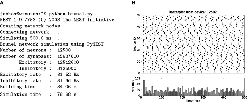
Figure 5. Results of the balanced random network simulation. (A) The transcript of the simulation session shows the output during network setup and the summary printed at the end of the simulation. (B) Spike raster (top) and spike time histogram (bottom) of the
.
N_rec recorded excitatory neuronsThe authors declare that the research was conducted in the absence of any commercial or financial relationships that could be construed as a potential conflict of interest.
We are grateful to our colleagues in the NEST Initiative and the FACETS project for stimulating discussions, in particular to Hans Ekkehard Plesser for drawing our attention to the visitor pattern. Partially funded by DIP F1.2, BMBF Grant 01GQ0420 to the Bernstein Center for Computational Neuroscience Freiburg, EU Grant 15879 (FACETS), and “The Next-Generation Integrated Simulation of Living Matter” project, part of the Development and Use of the Next-Generation Supercomputer Project of the Ministry of Education, Culture, Sports, Science and Technology (MEXT) of Japan.
Plesser, H. E., Eppler, J. M., Morrison, A., Diesmann, M., and Gewaltig, M.-O. (2007). Efficient parallel simulation of large-scale neuronal networks on clusters of multiprocessor computers. In Euro-Par 2007: Parallel Processing, Volume 4641 of Lecture Notes in Computer Science, A.-M. Kermarrec, L. Bouge, and T. Priol, eds (Berlin, Springer-Verlag), pp. 672–681.
van Rossum, G. (2008). Python/C API Reference Manual. Available at: http://docs.python.org/api/api.html.