Universal Time variations in the magnetosphere

1 Introduction

The first description of a Universal Time (UT) variation in global geomagnetic activity, that we know of, was by Bartels (1925) and Bartels (1928) who postulated that the variation was linked to the angle of tilt ψ of Earth’s magnetic axis relative to the sunward (X) direction. Bartels studied the “U index” which commenced in 1835 and was continued until the 1930s. Until 1871, this index was based on declination readings from just two magnetic observatories, after which it was based on seven stations (Russell and McPherron, 1973; Nevanlinna, 2004). The U index is equivalent to the magnitude of the difference between successive daily averages of the modern Dst index. In their book, Chapman and Bartels (1940) commented (Sect. XI. 20, p. 391), “since the local time of Batavia and Potsdam differ by 5–6 h, the identity of the hours of maximum or minimum U suggests the existence of a “Universal Time” variation of U. Such a variation might depend, for example, on the varying angle between the Earth’s magnetic axis and the line connecting the Sun and the Earth”. This idea is now usually referred to as “dipole tilt effects” or the “equinoctial hypothesis”.

In the century since Bartels’ original deduction, a very large number of papers have discussed UT variations in the magnetosphere which, given that many magnetospheric processes take place in limited magnetic local time regions (in particular, substorm phenomena take place in the sector around local midnight), gives potential longitudinal variations in space weather and also means that the effects of a given disturbance in interplanetary space depend upon its time of arrival at Earth. UT variations have been reported in geomagnetic indices in a great many studies (Waldo-Lewis and McIntosh, 1953; McIntosh, 1959; Nicholson and Wulf, 1961; Davis and Sugiura, 1966; Berthelier, 1976; Aoki, 1977; Mayaud, 1978; Russell, 1989; Berthelier, 1990; Saroso et al., 1993; Takalo et al., 1995; de La Sayette and Berthelier, 1996; Siscoe and Crooker, 1996; Hajkowicz, 1998; Ahn et al., 2000; Cliver et al., 2000; Lyatsky et al., 2001; O’Brien and McPherron, 2002; Ahn and Moon, 2003; Karinen and Mursula, 2005; Wang and Lühr, 2007; Yakovchouk et al., 2012; Chu et al., 2015; Lockwood et al., 2020a; Lockwood et al., 2020b; Lockwood et al., 2020c; Balan et al., 2021; Lockwood et al., 2021; Wang et al., 2021). A problem for all these studies is that if the longitudinal distribution of magnetometer stations employed is not even, then a spurious UT variation is introduced into the geomagnetic data (Mayaud, 1978; Mayaud, 1980; Takalo and Mursula, 2001; Lockwood et al., 2019b). This is a particular problem in the Southern hemisphere where the oceans limit the locations at which magnetometers can be installed and operated. As a result, the majority of geomagnetic indices are generated using data from stations that are either equatorial or in the northern hemisphere. This introduces further seasonal complications and others associated with north-south asymmetries in the intrinsic main field of Earth. In theory, space-based observations could be able to avoid these issues, but care must be taken using both in-situ and remote-sounding satellite data because there are always orbit considerations that mean UT variations can arise from sampling and aliasing with other variations (for example, local time, latitudinal, annual, solar cycle). We here exploit the opportunities presented by long-duration datasets and by swarms of satellites to minimise such issues. In particular, we use the Active Magnetosphere and Planetary Electrodynamics Response Experiment (AMPERE) analysis of data on field-aligned currents from magnetometers on board more than 70 Iridium satellites in circular low-Earth orbit (altitude 780 km) in six orbit planes, which give 12 cuts at different values of MLT in each orbit through the auroral oval (Anderson et al., 2014; Milan et al., 2015). This has already allowed studies of UT variations in the field-aligned currents that bring energy and momentum from the magnetosphere to the ionosphere and drive geomagnetic activity (Coxon et al., 2016; Sangha et al., 2022).

1.1 Earth’s eccentric magnetic field

Figure 1 shows the locations of three types of magnetic pole in the two hemispheres of Earth and how they have varied over time. The orange points are the dip poles, defined as where the magnetic field is vertical. The dip pole locations vary with currents that flow in the ionosphere as well as the internally-generated main field and their location has drifted considerably further than poles of other definition. The blue dots are the poles for a geocentric dipole fitted to the observations, being the 12th. generation of the International Geomagnetic Reference Field (IGRF) for 1900 to 2020 (Thébault et al., 2015). Note that for the geocentric dipole poles, the offsets from the rotational pole are the same in the two hemispheres and that they are always separated by 180° of longitude. The drift of these poles is considerably smaller than for dip poles. The mauve points are for eccentric dipole fits to the data for after 1980 by Koochak and Fraser-Smith (2017). In this fit, the dipole axis is not constrained to pass through the centre of the Earth. Coefficients to compute the pole locations (the eccentric dipole axial poles, where the dipole moment threads the Earth’s surface) are only available for 1980 onwards. In that time, the north pole of the eccentric dipole has moved closer to the rotational axis, whereas the southern pole has migrated away from it. In addition, the longitude difference has decreased further. Förster and Cnossen (2013) noted that these hemispheric field differences were probably more important for polar thermospheric neutral winds than ionospheric plasma convection but can still influence currents, convection and power dissipation rates in the upper atmosphere and the hemispheric field differences have implications that have been invoked by Laundal et al. (2017) and are discussed further in this paper.

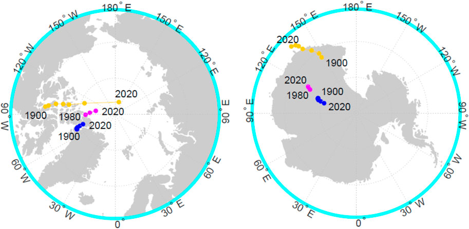
FIGURE 1. Maps of the magnetic pole locations in the (left) Northern and (right) Southern hemispheres at dates 20 years apart. The orange and blue points are dip and geocentric dipole pole locations from the International Geomagnetic Reference Field (IGRF, 12th. generation) (Thébault et al., 2015). Points are shown for 1900 to 2020 in steps of 20 years. The mauve points are the axial poles for the years 1980, 2000, and 2020 from the eccentric dipole model fits (in which the dipole axis is not constrained to pass through the centre of the Earth) of Koochak and Fraser-Smith (2017).

1.2 Pole motions in a “geocentric-solar” frame of reference

Lockwood et al. (2021) have noted the relevance to UT variations in the magnetosphere-ionosphere system of the diurnal motions of the magnetic poles in a geocentric-solar frame. By this we mean a frame with its origin at the centre of the Earth and an X-axis that points from there to the centre of the Sun. Thus GSEQ (Geocentric Solar Equatorial), GSE (Geocentric Solar Ecliptic) and GSM (Geocentric Solar Magnetospheric) are all examples of such frames. For GSEQ and GSE the magnetic poles follow paths that are close to circular every day (Lockwood et al., 2021) but for GSM the loci are generally elliptical with the same motion in the X direction but changes to the motion in the Y direction introduced by the rotation of the GSM Y- and Z-axes around the X-axis (so as to make the Z-axis antiparallel to the projection of Earth’s magnetic axis $\vec{M}$ onto the YZ plane).

For the axial poles of an eccentric dipole model of Earth’s field, the greater offset of the rotational and magnetic poles in the Southern hemisphere causes these motions to be of greater radius and speed in the southern hemisphere than the northern, and the two are not precisely in antiphase. A key point about these pole motions is that, to a large extent, the ionospheric polar caps show the same motions as the poles themselves: this is revealed by both by observations (Stubbs et al., 2005) and geomagnetic field modelling (Tsyganenko, 2019) of the auroral oval and the polar cap. The papers by Lockwood et al. (2021) and Lockwood et al. (2022) detail a variety of observational studies that show that the polar caps and auroral ovals reflect, almost entirely, the motions of the poles. This is also replicated in global MHD modelling of the magnetosphere with dipole tilt effects (Kabin et al., 2004; Lockwood et al., 2020c). Note however, that simulations have almost exclusively used a geocentric dipole field rather than an eccentric one.

Figure 2 shows the magnetosphere at four UTs and at equinox (although the time-of year is not relevant in this context as it has little effect on the diurnal variations in the speed of sunward/antisunward motion). Because the poles are less than 180° apart, the North pole is at its most antisunward at 6.71 h UT while the South pole is at its most sunward at 4.18 h UT (These times are derived using the eccentric dipole field model of Koochak and Fraser-Smith (2017) for the year 2016). Figure 2A is for around 5 h UT, when the poles are near these extremes. Conversely, the North pole is at its most sunward at 18.71 h UT while the South pole is at its most antisunward at 16.17 h UT and Figure 2C is for around 17 h UT. Between these times, at 11 h UT (Figure 2B) the North pole is close to its fastest speed of sunward motion (V_P = V_NP = +47.8 ms⁻¹) and the South pole close to its fastest speed of antisunward motion (V_P = V_SP = −127.5 ms⁻¹). At 23 h UT (Figure 2D) the motions are in the opposite direction completing the diurnal cycle.

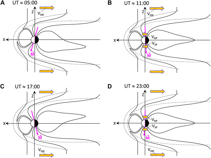
FIGURE 2. Schematics of pole motions in a geocentric-solar frame (i.e., one fixed with respect to both the Earth and the Sun). The panels show the magnetosphere in the noon-midnight (XZ) plane at (A) near 05 h UT; (B) near 11 h UT; (C) near 17 h UT; and (D) near 23 h UT at equinox. The mauve arrow shows Earth’s magnetic axis $\vec{M}$. Note that, by convention, the north/south pole of a magnet is where field lines diverge/converge and so for the current polarity of the geomagnetic field, the magnetic pole in the southern hemisphere is, by that convention, a north magnetic pole and vice versa: in this paper, we refer to a magnetic pole by the hemisphere of the Earth that it is in and not by the magnet convention. The mauve arrow shows the magnetic moment of an eccentric dipole. The dot-dashed lines are the magnetopause and the dashed lines the bow shock. Outside the bow shock the solar wind flows in the −X direction at speed V_SW. At around 05 h UT the “north” magnetic pole (i.e., the magnetic pole in the northern hemisphere) is pointed away from the Sun and the “south” magnetic field is pointed toward it. At around 17 h UT the north/south magnetic pole is pointed toward/away from the Sun. At around 11 h UT the north/south magnetic pole is moving toward/away from the Sun and at around 23 h UT the north/south magnetic pole is moving away from/toward the Sun. The sunward component of the motion of the north/south magnetic pole at ionospheric F-region altitudes in any geocentric-solar frame is V_NP and V_SP, respectively.

These pole motion speeds appear to be negligible when in the context of the solar wind speed V_SW which is of order 500 kms⁻¹ in the same geocentric-solar frame; however, they are not negligible when we consider the consequent electric fields and voltages (i.e., magnetic flux transport rates): the southward, flow-perpendicular, field B_Z in the solar wind is typically 5 nT giving a dawn-dusk electric field E_Y = B_ZV_SW∼2.5 mVm⁻¹, whereas in the ionosphere the field is B_i ≈ 5 × 10⁵T so the pole motions yield dawn-dusk polar cap electric fields in the ionosphere that peak at B_iV_P ≈ 2.4 mVm⁻¹ and ≈6.4 mVm⁻¹ in the north and south polar caps, respectively. In terms of voltage, for a polar cap latitudinal radius of 13° (giving a polar cap diameter at 400 km altitude of d_PC = 3,100 km), this yields peak transpolar voltage contributions of order 8 kV and 19 kV in the North and South polar caps.

To understand the implications of these pole motions in a geocentric-solar frame, consider Figure 3. When the polar cap is moving sunward it will reduce the transpolar voltage (the voltage associated with antisunward flow in the polar cap) and hence reduce the directly-driven power deposition in the polar and auroral ionosphere and thermosphere. The antisunward convection speed in the polar cap of the open flux tube F, V_i, is reduced; however, the segment of the open flux tube in interplanetary space is flowing at supersonic and super-Alfvénic speeds antisunward and away from the polar cap. It therefore can have no information about what is happening at its footpoint and is unaffected by it. We call the region of open flux in interplanetary space the “Stern Gap” (SG in Figure 3) and it has a width in the Y-dimension of L_SG across which the voltage is Φ_SG = L_SGB_ZV_SW, where B_Z is the southward component of the Interplanetary Magnetic Field (IMF) and V_SW the solar wind speed, both of which remain constant for each open flux tube as it propagates antisunward. Applying Faraday’s law (in integral form) to the loop PASGUC (the dashed yellow line) the reduction in V_i will reduce the transpolar voltage Φ_PC = d_PCB_iV_i giving Φ_PC < Φ_SG. Without significant field-parallel electric fields, the voltages along the field aligned segments of the loop (AP and UC in the magnetosphere and SA and GU in the magnetosheath) are zero and so Φ_SG > Φ_PC means that, by Faraday’s law in integral form, the magnetic flux threading the loop is growing. In other words, what is happening is that the rate at which flux tubes are transferred across SG exceeds that at which they are transferred across PC and so the flux threading the loop increases. In the nightside magnetosheath, the antisunward flow is also supersonic and super-Alfvénic and so is also unaffected by the slowing of the footpoint F, hence the voltage in the magnetopause along AU is unchanged and the flux accumulation is therefore in the loop PAUC, i.e., in the tail lobe. Hence the sunward pole motion has reduced the directly-driven flow and energy deposition in the ionosphere but increased the rate of energy storage in the tail lobes. In the other half of the diurnal cycle, the antisunward motion of the pole would have the reverse effects.

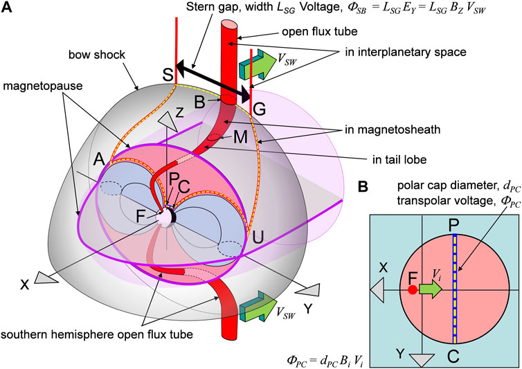
FIGURE 3. (A). Schematic of inductive decoupling of the “Stern Gap” voltage across open field lines in interplanetary space, Φ_SG and the transpolar voltage in the ionosphere Φ_PC. The magnetosphere is here viewed from northern middle latitudes in the mid-afternoon sector. The loops PASGUC (shown by the yellow dashed line) and PAUC (enclosing the northern tail lobe cross section shaded pink) are fixed in the XYZ GSM frame, where P and C are the dawn and dusk extremes of the northern ionospheric polar cap, AP and UC are field-aligned in the magnetosphere, SA and GU are field aligned in the magnetosheath, SG lies in the bow shock and AU in the tail magnetopause. The red flux tubes are open field lines and the northern-hemisphere tube threads the bow shock at B and the magnetopause at M and has an ionospheric footpoint, F. The solar wind flow is in the −X direction at speed V_SW. (B) Is a view looking down (in the −Z direction) on the northern hemisphere polar cap in which the antisunward ionospheric convection velocity of the footpoint F is V_i.

Such inductive decoupling of voltages in the solar wind and in the polar cap is a key component in the Expanding-Contracting Polar Cap (ECPC) model of the excitation of ionospheric convection which considers the effects of differences between the reconnection voltages in the dayside magnetopause (where open flux is generated) and in the cross-tail current sheet (where it is lost), Φ_D and Φ_N. (Holzer et al., 1986; Cowley and Lockwood, 1992; Lockwood, 1993; Milan et al., 2003; Lockwood and Morley, 2004; Milan, 2004; Milan et al., 2007; Milan et al., 2008; Milan et al., 2021; Lockwood and Cowley, 2022). The effect of pole motions illustrated in Figure 2 will add diurnal cycles to the accumulation and loss of lobe flux in substorm cycles associated with differences between Φ_D and Φ_N.

At first sight, it may appear that the voltage perturbations due to pole motions (computed above to be 8 kV and 19 kV for a typical polar cap radius in the north and south hemispheres, respectively) are small compared to the solar wind driving voltages Φ_SG and the reconnection voltages Φ_D and Φ_N, which can all exceed 100 kV or more. However, it is important to note that the pole-motion voltages are applied consistently for long periods, rising and falling sinusoidally over a 12-h period. This is in contrast to the voltage applied by the solar wind which usually fluctuates rapidly because of the rapid variations in the IMF orientation and only is consistently applied over similar timescales in large magnetic cloud and other CME impact events.

In order to quantify the effect of IMF orientation on various timescales, Figure 4 shows the distributions of estimated magnetopause reconnection voltage Φ_D for four different averaging periods. These are computed from the averages of 1-min observations of the interplanetary medium for 1995–2021, inclusive, using the optimum coupling function for transpolar voltage derived by Lockwood and McWilliams (2021a), using the 25-year data set from the SuperDARN radars of Lockwood and McWilliams (2021b) and evaluated during storm conditions by Orr et al. (2022). The interval 1995–2021 was chosen to minimise data gaps (Lockwood et al., 2019a). For the raw 1-min data shown in part A, the mode value is zero due to the large fraction of time that the IMF is sufficiently strongly northward. The mean value of all these distributions is 24 kV and the distributions narrow down to this mean as the length of the averaging interval τ is increased, according to the central limit theory. This means that the mode increases up toward this value with increasing τ and the median, 95- and 99-percentiles decrease toward it. For example for 12-h means (Figure 4D) the mode value is 17 kV and the median is 21 kV. These values are smaller than might initially be expected because of the large variability of the IMF orientation within the averaging intervals (Lockwood et al., 2019a; Lockwood, 2022) which means that the near-zero values due to strongly northward IMF are averaged in. In comparison, over the 12 h of sunward motion of a polar cap of diameter 3,100 km, the mean pole-motion voltages are 5 kV and 12 kV in the North and South polar caps. Perhaps the most pertinent comparison is for 2-h intervals, which is the duration of a longer substorm growth phase (Li et al., 2013; Partamies et al., 2013). The mode value of the distribution of estimated Φ_D is 15 kV (Figure 4C) whereas the peak values of ϕ_N and ϕ_S are 8 kV and 19 kV, respectively. We conclude that, compared with typical values of magnetopause reconnection voltage over extended intervals, the voltages associated with pole-motions are certainly not negligible.

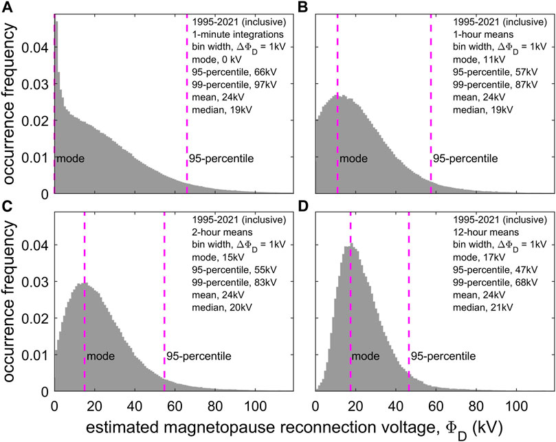
FIGURE 4. Distributions for different averaging intervals of estimates of the dayside reconnection voltage Φ_D from upstream interplanetary measurements, using the optimum coupling function for transpolar voltage derived by Lockwood and McWilliams (2021a). (A) 1-min raw data; (B). 1-h averages; (C). 2- averages; (D) 12-h averages. The mean value of these distribution is 24 kV and in each case the mode, the median and the 95- and 99-percentiles are given.

Figure 5 shows the waveforms of the pole-motion variations for a nominal polar cap diameter d_PC of 3,100 km (latitudinal polar cap radius Λ_PC = 13°). These variations are computed using the eccentric dipole field model of Koochak and Fraser-Smith (2017) for the year 2016. For a geocentric dipole, the average of the two would be zero (North and South variations would be of equal amplitude and in antiphase) and UT effects would be hemispheric only and not global. However, for the eccentric dipole there is considerable UT variation for the average of the two hemispheres. In each panel, the red line (with red circle symbols) is for the northern hemisphere, the blue line (with blue square symbols) for the southern and the black line (with black triangle symbols) the average of the two. This color and symbol coding is used throughout this paper for north, south and the global average: note that the symbols are there to aid readers with impaired color vision and are not at the temporal resolution of the data. The sunward/antisunward motion of a pole (positive/negative V_P, respectively, in Figure 5A) corresponds to a voltage ϕ = f_cd_PCB_iV_P, where B_i is the ionospheric magnetic field, d_PC the dawn-dusk polar cap diameter, and f_c allows for factors such as any change in shape of the polar cap. For a positive V_P (and hence ϕ), the polar cap voltage Φ_PC is reduced, as shown in Figure 5B, but as demonstrated by Figure 3, this means that the rate of addition to the lobe flux in that hemisphere, dF_lobe/dt is increased by ϕ, as shown in Figure 5C. Integrating ϕ over time gives the modulation to the lobe flux ΔF_lobe shown in Figure 5D. In part D all variations are shown with respect to their respective minimum values in their diurnal cycle.

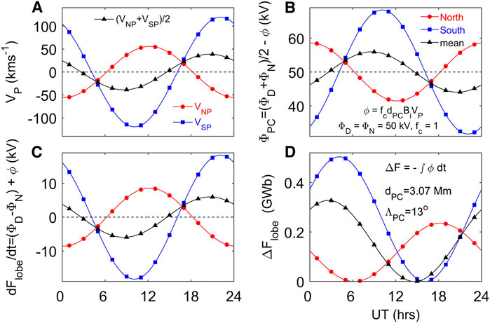
FIGURE 5. Analysis of the effect of pole motions in a geocentric-solar frame for a nominal polar cap diameter d_PC of 3100km, computed using the eccentric dipole field model of Koochak and Fraser-Smith (2017) for the year 2016. (A) The sunward velocity V_P, of the north (V_NP, in red with red circle sympols) and south (V_SP, in blue with blue square symbols) poles. The black line (with black triangle symbols) is the average of the two. (B) The corresponding variations in the transpolar voltages Φ_PC due to the perturbation by pole motions ϕ = f_cd_PCB_iV_P. This example is for reconnection voltages in the dayside magnetopause (Φ_D) and nightside cross tail current sheet (Φ_N) of 50 kV and Φ_PC = (Φ_D + Φ_N)/2 − ϕ. The fraction of the voltage ϕ that is applied to the polar cap is here f_c = 1. (C) The corresponding rate at which flux is added to the tail lobe dF_lobe/dt = (Φ_D − Φ_N) + ϕ. (D) The integral flux ΔF added to the lobe with respect to the minimum of the diurnal cycle in each case. ΔF_N (in red with red circle symbols) is added to the northern lobe with minimum at 0.47 h UT and maximum of 0.2 GWb at 12.47 h UT; ΔF_S (in blue with blue square symbols) is added to the southern lobe with minimum at 10.17 h UT and maximum of 0.49 GWb at 12.17 h UT; the average of the two is ΔF_M = (ΔF_N + ΔF_S)/2 (in black with black triangle symbols) has a minimum at 14.86 h UT and maximum of 0.34 GWb at 2.86 h UT. Note that the total flux added to the tail is 2ΔF_M and peaks at a maximum of 0.68 GWb. Note also that each line in part (D) is the flux relative to its own minimum value which is different for all three lines.

The change in the total tail flux (in both lobes) is 2ΔF_NS, where F_NS = (F_N + F_s)/2. This change in total lobe flux is at a minimum at 14.86 h UT after which it increases reaching a maximum of 0.68 GWb 12 h later at 2.86 h UT. In that interval, the directly driven flows and currents in the ionosphere will be reduced while the energy stored in the lobe increases. To put these lobe flux changes in context we can compare with estimates of the polar cap flux F_PC, which is equal to the tail lobe flux plus the relatively small open flux that threads the dayside magnetopause (Lockwood et al., 2021). Values of F_PC reported in the literature vary between about 0.1 GWb and 1.2 GWb. The lowest estimate that we know of is 0.08 GWb during a northward-IMF “horse collar” aurora event (Wang et al., 2023) and it has been argued that F_PC saturates at 1.2 GWb during major geomagnetic storms (Mishin and Karavaev, 2017). Kamide et al. (1977), Boakes et al. (2009) and Milan et al. (2008) find that substorm onset becomes more likely when F_PC is increased: Boakes et al. (2009) found the probability of an onset to be negligible for F_PC below 0.3 GWb but above this value increased linearly with F_PC. Substorm onsets are typically initiated when F_PC reaches about 0.9 GWb but larger values, up to about 1.1 GWb, have been deduced in sawtooth events and steady convection events (DeJong et al., 2007; Lockwood et al., 2009; Brambles et al., 2013).

Hence the pole motions could be a significant factor in modulating the probability that a substorm commences. In addition, it could potentially modulate how strong a disturbance it develops into once it has begun. Note that between 0.34 and 14.86 h UT the total tail lobe flux is being reduced and transpolar voltage and power deposited in the ionosphere increased, independent of any nightside reconnection. This effect peaks at about 07:30 UT.

1.3 Ionospheric conductivity effects

The motion of the poles has a second effect, namely it changes the solar zenith angles at locations inside the polar caps and auroral ovals, thereby modulating the EUV-generated ionospheric conductivities at those locations. This effect has been invoked many times in the context of UT variations in geomagnetic activity (Lyatsky et al., 2001; Newell et al., 2002; Wang and Lühr, 2007).

Enhanced conductivity, generated by solar EUV illumination, peaks when the polar cap is tipped toward the Sun (Ridley et al., 2004). Hence there is a phase difference of π/4 between EUV-induced conductivity effects and the pole-motion effects discussed in the previous sub-section, the latter peaking 6 h earlier when the pole is tipping toward the Sun at its fastest rate. A complication with conductivity effects is that solar EUV is not the only source of enhancement because particle precipitation, particularly in the auroral ovals, also increases the ionospheric conductivities; this is highly variable and in certain places and times is dominant over the EUV source (Kubota et al., 2017). This second source of conductivity is strongly ordered by Magnetic Local Time (MLT) and although given events show strong UT variations as the event evolves (for example during storms or substorm cycles), those events are largely random in the UT of their occurrence and so regular, systematic UT variations are hard to define (Carter et al., 2020). We have had good models of EUV-generated conductivity for many years [e.g., Brekke and Moen (1993)] but the variability, in time and space, of precipitation-induced conductivity has made the development of equivalent models much more difficult and complex (Zhang et al., 2015; Carter et al., 2020).

The effect of enhanced conductivity in a polar cap is very similar to that of motion of the pole toward the Sun because the antisunward ionospheric flow speed is reduced in that polar cap (Ridley et al., 2004) whilst being enhanced in the other polar cap by the lower conductivity (so this is similar to the inductive effect of the pole motion). This effect is seen in “saturation”, in which enhanced conductivity gives rise to lower-than-expected transpolar voltages when solar wind-magnetsophere coupling is exceptionally strong and even makes them tend asymptotically to an upper limit (Russell et al., 2001; Hairston et al., 2003; Shepherd, 2007; Orr et al., 2022). Something that cannot be overlooked when considering conductivity effects is the need to be consistent when evaluating the roles of ionospheric conductivity and flux transport, a need that is imposed by Maxwell’s equation $\nabla \cdot \vec{B}=0$. This fundamental equation of electromagnetism (the non-existence of magnetic monopoles) demands that the open flux in the two hemispheres must be identical at any instant (because open flux is only generated and lost by magnetic reconnections which change the open flux in both hemispheres by the same amount). In addition, when integrated/averaged over sufficient time, the antisunward magnetic flux transport rate of open flux in both ionospheric polar caps (i.e., the transpolar voltages) must both be the same as that of the parts of the open field lines that are in interplanetary space. This consideration leads to many of the proposed mechanisms for explaining saturation effects invoking a mechanism that imposes a limitation to the reconnection voltage at the dayside magnetopause (Siscoe, 2002). This means that the voltage would be reduced equally in both polar caps by enhancements to the conductivity in either polar cap.

An alternative explanation of saturation effects is provided by inductive effects which reduce the flow in only the polar cap in which the conductivity is enhanced. However, such a mechanism can only smooth out peaks and troughs in the reconnection voltage such that the enhancement/decrease in transpolar voltage is smaller but lasts longer. Were this not the case, long-term averages of the transpolar voltage in the two polar caps would differ and differ from the average rate of anti-sunward flux transport of open flux in interplanetary space, which would violate $\nabla \cdot \vec{B}=0$. Several numerical simulations confirm that increased polar cap conductivity reduces transpolar voltages on shorter timescales (Raeder et al., 2001; Merkine et al., 2003; Borovsky et al., 2009; Kubota et al., 2017). This is to be expected because field-perpendicular conductivity (both Hall and Pedersen) arise from collisions between ions and electrons and neutral atoms and these collisions also give frictional drag on the motion of F-region plasma and frozen-in magnetic field (Ridley et al., 2004). As discussed by Tanaka (2007) and (for an isolated flux tube) by Southwood (1987), this is the “line-tying” concept introduced by Atkinson (1967); Atkinson (1978) to explain the origin of field-aligned currents and how they transfer momentum and energy down into the ionosphere. Because the interplanetary segments of open field lines, outside the bow shock in the “Stern gap”, and indeed in the tail magnetosheath, are flowing supersonically and super-Alfvénically away from the ionospheric polar cap that they are connected to, they can have no information about the state of the ionosphere and so are not influenced in any way by the slowing of their field line footpoints. Over short intervals the changes can be in the dayside magnetosheath (Pulkkinen et al., 2016) but over the timescales over which field lines are transferred to the nightside of Earth, the sheath flow becomes super-sonic and super-Alfvénic and the changes then must be increasingly inside the tail lobe. Hence the reduction in transpolar voltage associated with enhanced polar cap conductivity must, like the effect of a sunward-moving pole, give induction effects in the field of the relevant tail lobe between the ionosphere and the tail magnetopause and hence a rise in the energy stored in that tail lobe. Indeed, in the MHD simulation of the Bastille day storm by Raeder et al. (2001), the lobes swell so much that the magnetospheric shape becomes distorted. This means that enhanced conductivity is really influencing the balance between energy stored in the tail (and later released) and energy directly deposited in the ionosphere. This explanation of conductivity effects can therefore influence the transpolar voltage in one polar cap but not the other; but note that, unless one is invoking magnetic monopoles (which have never been definitively detected), this effect must average out on long timescales.

We here model the diurnal variations of EUV-induced ionospheric height-integrated Pedersen conductivity using the eccentric dipole model. We use the variation of Pedersen conductivity with solar zenith angle by Ridley et al. (2004), shown in their Figure 2. We compute the UT and F variations of zenith angle at points separated by 1° in both latitude and longitude and then average them over three regions: the polar cap, the dayside auroral oval and the nightside auroral oval. The polar cap is assumed circular with an angular geocentric radius of 13°, centred 5° to the antisunward side of the geomagnetic pole. The auroral oval is between this and another circle of angular radius 17°, centred 6° antisunward of the geomagnetic pole. The dayside/nightside oval is sunward/antisunward of the geomagnetic pole.

Figure 6 shows the fraction-of-year (F)- Universal Time (UT) patterns of the EUV-generated, height-integrated ionospheric Pedersen conductivity, Σ_p. Beside each color plot is a plot of the mean Σ_p (averaged over all times of year) against UT. These patterns are similar to those published before, but the eccentricity in the magnetic field can be seen in the contours for the southern hemisphere, which are less aligned with the vertical than they are for the northern hemisphere. The line plots also show the UT variations are not quite the sine waves that are predicted by a geocentric dipole.

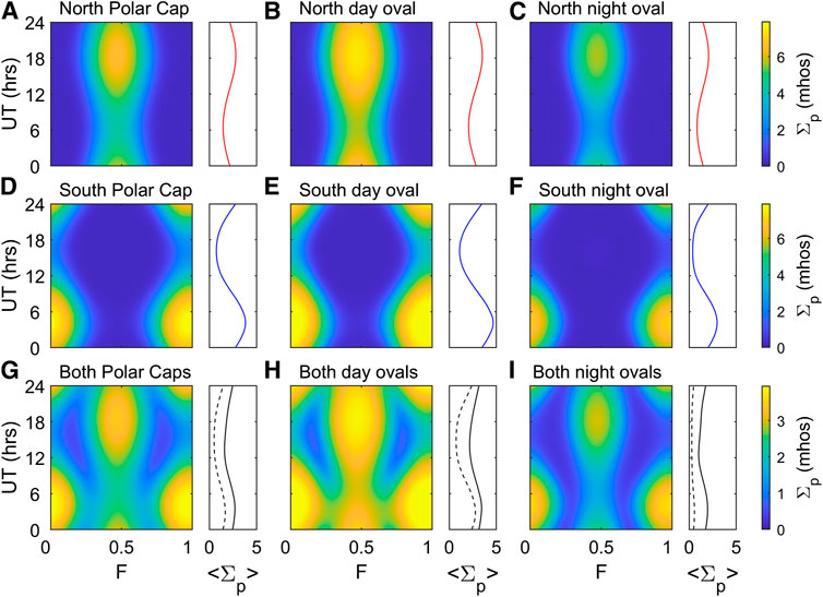
FIGURE 6. Analysis of the effect of pole motions on solar EUV-generated, height-integrated ionospheric Pedersen conductivity, computed using the dependence on solar zenith angle by Ridley et al. (2004) and the eccentric dipole model of Earth’s magnetic field by Koochak and Fraser-Smith (2017) for the year 2016. The variations of mean Pedersen conductivity are color-coded as a function of fraction of the year (F, horizontal axis) and Universal Time (UT, vertical axis). To the right of each color plot is a plot of the mean height-integrated Pedersen conductivity ⟨Σ_p⟩ (averaged over all times-of-year, F) as a function of UT. Plots are for three regions (see text for full definitions): the left-hand column (part (A,D,G)) is for the polar cap, the middle column (part (B,E,H)) for the dayside auroral oval and the right-hand column (part (C,F,I)) for the nightside auroral oval. The top row is for the northern hemisphere, the middle row for the southern hemisphere and the bottom row for the average of both hemispheres. The dashed black lines in the bottom row of ⟨Σ_p⟩ - UT plots show the minimum value at that UT.

1.4 The McIntosh pattern

The time-of-year/time-of-day (F-UT) plots of conductivity in both hemispheres shown in the bottom row of Figure 6 display what is known as the “equinoctial” or “McIntosh” pattern. This pattern follows the contours in a F-UT plot of values of the dipole tilt angle ψ close to 90° (equivalent to μ near zero - these angles are defined below). This pattern is also seen in geomagnetic activity (McIntosh, 1959). The low-conductivity bands coincide with when geomagnetic activity is enhanced (Berthelier, 1976; de La Sayette and Berthelier, 1996; Cliver et al., 2000; Lockwood et al., 2020a; Lockwood et al., 2021). It should be noted here that the equinoctial pattern is most clearly seen in the am index, compiled from homogeneous rings of mid-latitude stations, which are range indices which respond primarily to the substorm current wedge (Menvielle and Berthelier, 1991).

Lyatsky et al. (2001) and Newell et al. (2002) propose that the low EUV-generated conductivity in the nightside auroral oval of both hemispheres causes larger substorm expansions, and hence greater geomagnetic activity. The reasons why this might be the case are qualitative and the physical mechanism unclear and there are several other proposed causes: these include the stability of the near-Earth tail (Kivelson and Hughes, 1990) and dipole tilt effects on the magnetopause reconnection voltage Φ_D (Crooker and Siscoe, 1986; Russell et al., 2003).

Finch et al. (2008) analysed the F-UT patterns in data from a very large number of individual magnetometer stations and showed that the equinoctial pattern arises in the nightside auroral oval. These authors specifically found it to be absent in dayside stations. Similarly, Lockwood et al. (2020b) and Lockwood et al. (2020a) used the mid-latitude aσ indices, which cover 6-h ranges in Magnetic Local Time (MLT) and showed the equinoctial pattern was strongest in the midnight sector but hardly detectable in the noon sector. This argues against the equinoctial pattern being generated by dipole tilt effects on dayside magnetopause coupling and the magnetopause reconnection voltage Φ_D as proposed by Crooker and Siscoe (1986) and Russell et al. (2003).

These results strongly indicate that the equinoctial pattern in indices such as am is not consistent with dipole tilt modulation of the reconnection rate in the dayside magnetopause. However, this does not mean that such effects do not occur and numerical simulations by global MHD models have found dipole tilt modulation of magnetopause reconnection voltage (Eggington et al., 2020). It is important to note that Eggington et al. (2020) define a dipole tilt angle, μ, differently from the way it is defined in several other papers (Cliver et al., 2000; O’Brien and McPherron, 2002), which is here termed ψ: ψ is defined as the acute angle between the dipole axis and the X-axis of the geocentric-solar frames. For the Earth ψ varies between 56° and 90°. In fraction-of-year (F) against Universal time (UT) plots ψ shows the equinoctial pattern with the high-activity bands (around the equinoxes) coinciding with the contours of ψ close to 90° (giving the low Σ_p bands seen in the bottom row of Figure 6).

Eggington et al. (2020) define μ to be the angle that the dipole axis makes with the normal to the ecliptic plane which for Earth varies between −34° and +34° and μ = 0 corresponds to ψ = 90°. Hence, to explain the equinoctial pattern as the effect of dipole tilt on magnetopause reconnection voltage requires that Φ_D be a maximum for μ = 0. Figure 7A of Eggington et al. (2020) shows that this is not what the simulations predict. This plot covers |μ| up to 90°, but only the range −34 to +34° applies to the Earth. In this plot Φ_D increases with |μ| as it is increased from 0° to 10°, but it then decreases again but still remains higher than for μ = 0 for all values that apply to Earth |μ| < 34°. Hence the modelled dipole tilt effect on Φ_D is in the wrong sense to explain the equinoctial pattern of enhanced geomagnetic activity.

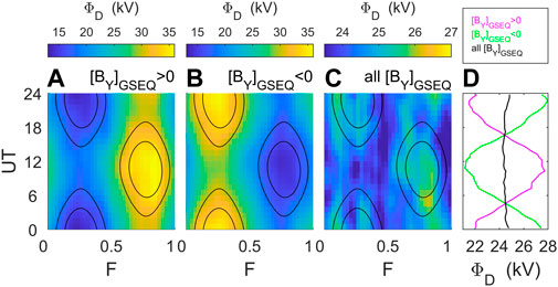
FIGURE 7. The Russell-McPherron effect seen in fraction of year (F) - Universal Time (UT) plots. The colors in parts (A), (B) and (C) are the mean predicted magnetopause reconnection voltage Φ_D generated using interplanetary data from 1996–2021, inclusive. The black contours are for 95% and 85% of the peak of the predicted IMF orientation factor in Φ_D (namely sin^2.5 (θ/2), where θ is the IMF clock angle in the GSM frame) for the simplified demonstration of the R-M effect in which the Z-component of the IMF in the GSEQ frame is zero. These contours are computed are for the R-M effect for the two Y-component polarities using an eccentric dipole model for the mid-point date of the data interval (i.e., for 2008). The data are sorted into (A) positive, (B) negative and (C) all ${[B_Y]}_{\mathit{GSEQ}}$. Note that the range of the color scale for part (C) is much smaller than for (A) and (B). Part (D) shows line-plots of the net UT variations in Φ_D, averaged over all F.

In this context, the plots in Figure 6 of conductiviies for the eccentric dipole are significant. The most uniform of geomagnetic indices, in terms of its F-UT response is am, by virtue of the great uniformity of the rings of magnetometer stations in both hemispheres employed in its construction (Lockwood et al., 2019b). This clearly shows an equinoctial pattern, very like that in Figure 6H, in which there is a net UT variation as well as an equinoctial pattern (Berthelier, 1976; de La Sayette and Berthelier, 1996; Cliver et al., 2000; Lockwood et al., 2020a; Lockwood et al., 2020b; Lockwood et al., 2021). However, the most relevant plot for the theory of Lyatsky et al. (2001) and Newell et al. (2002) is Figure 6I, being that for the nightside auroral oval. This plot shows an equinoctial pattern but with very little UT variation in the mean Σ_p (the solid black line) and essentially none in the minimum Σ_p (the dashed black line). Thus the mechanism proposed by Lyatsky et al. (2001); Newell et al. (2002) explains the equinoctial pattern but not the overall variation with UT, whereas a mechanism invoking EUV-generated conductivity in the polar cap or dayside auroral oval (shown in Figures 6G, H, respectively) could explain the observed net UT variation as well as the equinoctial pattern.

1.5 Tail warping effects

Ionospheric conductivity in both ionospheres is not the only relevant parameter to show the equinoctial F-UT pattern and hence a dipole tilt dependence. Another is the “hinge angle” between the mid-tail (which is aligned with the solar wind) and the near-Earth tail (which is ordered by Earth’s magnetic axis). Kivelson and Hughes (1990) proposed that this angle plays a role in the stability of the tail and the triggering of substorm onsets, an idea investigated further by a number of authors (Danilov et al., 2013; Kubyshkina et al., 2015; Korovinskiy et al., 2018; Kubyshkina et al., 2022). A variant of this idea was proposed by (Alexeev et al., 1996) who suggested the dipole tilt effect was through a change in the proximity of the ring current and the closest auroral electrojet. The dipole tilt effect of ring current latitude was also invoked by Ou et al. (2022) as a cause of hemispheric differences in geomagnetic disturbance.

The study of Finch et al. (2008) showed that stations whose location (in an MLT-magnetic latitude frame) yielded an equinoctial pattern also showed a response that depended on the square of the solar wind velocity, whereas stations at locations which did not give an equinoctial pattern did not. This was one reason why Lockwood (2013) proposed that the equinoctial pattern arose from the role of solar wind dynamic pressure in compressing the near-Earth geomagnetic tail at X coordinates where the tail is flaring (i.e., where the radius of cross section is increasing with -X). Furthermore, Lockwood et al. (2020a) showed that the amplitude of the equinoctial pattern in geomagnetic activity increased with solar wind dynamic pressure, which suggests that the squeezing of the near-Earth tail by dynamic pressure is important in the generation of the equinoctial pattern. Using an empirical model of magnetopause positions and a global MHD model of the magnetosphere, Lockwood et al. (2020c) showed that the equinoctial pattern could indeed arise from the effect that dipole tilt has on pressure balance in the near-Earth tail. The reason is the latitudinal movement of the magnetopause reconnection site with dipole tilt, as first suggested from numerical simulations by Russell et al. (2003) and has been reproduced in a great many other model simulations (Park et al., 2006; Liu et al., 2012; Lu et al., 2013; Lockwood et al., 2020c; Eggington et al., 2020; Guo et al., 2020). This effect has also been observed using data from the Geotail and Magnetospheric Multiscale (MMS) mission spacecraft (Kitamura et al., 2016). A key consequence of this is that field lines in the hemisphere tipped away from the Sun evolve into the tail lobe faster than those in the hemisphere tipped toward the Sun (Lockwood et al., 2020c): this is partly because they have less distance to travel and partly because initially the magnetic tension force and the sheath flow both propel them into the tail, whereas initially the sheath flow and tension force are in opposition for the newly-opened field lines in the hemisphere tipped towards the Sun. On the dayside, this increases the pressure in the lobe of the hemisphere that is tipped toward the Sun (Hoilijoki et al., 2014), but reduces it in the near-Earth tail in that hemisphere (Lockwood et al., 2020a). The solar wind dynamic pressure compresses the tail to a greater extent, increasing the magnetic shear across the cross-tail current sheet, when μ is small (i.e., ψ is near 90°). The global MHD modelling presented by Lockwood et al. (2020c) shows that this can explain the observed dependence of the equinoctial pattern on solar wind dynamic pressure.

1.6 The Russell-McPherron effect and the influence of the IMF Y-component

There is another factor that it is very important to consider. The Russell-McPherron (R-M) effect (Russell and McPherron, 1973) is a fundamental mechanism in solar-wind magnetosphere coupling that is central to understanding the semi-annual variation in geomagnetic activity. A review of the evidence for this mechanism and of its influence has recently been given by Lockwood et al. (2020b,a). On its own, the R-M effect does not introduce a net UT variation; however, as explained below, if there are other UT effects and/or asymmetries it can amplify and modify them.

The R-M effect arises because the IMF is ordered, on average, in a solar frame (the Parker Spiral configuration) but coupling into the magnetosphere depends in its orientation relative to Earth’s magnetic dipole axis. The most appropriate solar frame is the Geocentric Solar Equatorial (GSEQ) in which the X-axis points from the centre of the Earth to the centre as the Sun (as in the GSE and GSM frames), Z is the northward normal to the solar magnetic equatorial plane and Y makes up the right-hand set. Hence GSEQ is similar to GSE, but is rotated by the 7° angle between the solar magnetic equatorial plane and the ecliptic. The key effect is that the Earth’s dipole tilt means that at the March equinox negative IMF ${[B_Y]}_{\mathit{GSEQ}}$ gives a southward IMF component in GSM (enhancing solar wind-magnetosphere coupling) whereas at the September equinox it is positive ${[B_Y]}_{\mathit{GSEQ}}$ that does this. Geomagnetic activity shows this preference for one equinox depending on the polarity of the ${[B_Y]}_{\mathit{GSEQ}}$ component very clearly and strongly (Zhao and Zong, 2012; Lockwood et al., 2020a; Lockwood et al., 2020b), confirming the key importance of the R-M effect.

Figure 7 shows the influence of the R-M effect on the predicted magnetopause reconnection rate Φ_D, computed from solar wind parameters using the optimum coupling function for transpolar voltage derived by Lockwood and McWilliams (2021a) from the 25-year dataset of SuperDARN radar data of Lockwood and McWilliams (2021b) [see also Lockwood (2022)]. This is computed using the relatively continuous interplanetary (Omni) dataset of 1-min resolution available since 1995 (King and Papitashvili, 2005; Lockwood et al., 2019a). The mean values of Φ_D are shown for A IMF ${[B_Y]}_{\mathit{GSEQ}}>+ϵ$, B ${[B_Y]}_{\mathit{GSEQ}}<-ϵ$ and C all ${[B_Y]}_{\mathit{GSEQ}}$, where ϵ is the standard error in the mean of all ${[B_Y]}_{\mathit{GSEQ}}$ (=0.0011 nT) Note that in parts (a) and (b) the means exclude the 1,023,833 1-min samples that are not significantly different from zero which yields 6,029,840 samples for ${[B_Y]}_{\mathit{GSEQ}}>+ϵ$ and 6,096,374 samples for ${[B_Y]}_{\mathit{GSEQ}}<-ϵ$. The two black contours are from the simplified demonstration of the R-M effect in which the IMF Z-component in GSEQ is taken to always have its mean value of zero (i.e., the field is in the average, Parker spiral configuration) and are predicted using tilt angles from the eccentric dipole field magnetic field model. These contours are at 95% and 85% of the peaks of the sin^2.5(θ/2) IMF orientation factor in the expression for Φ_D for the two IMF Y-component polarities in GSEQ. The angle θ is the IMF clock angle in the GSM frame and for the assumption of ${[B_Z]}_{\mathit{GSEQ}}=0$, this angle varies between (90–34) = 56° and (90 + 34) = 124° giving a variation in the sin^2.5(θ/2) IMF orientation factor between a minimum of 0.151 and a maximum of 0.733. The two peaks of this IMF orientation factor are at F = 0.2630 and UT = 22.75 h near the March equinox for ${[B_Y]}_{\mathit{GSEQ}}<0$ and at F = 0.7753 and UT = 10.50 h near the September equinox for ${[B_Y]}_{\mathit{GSEQ}}>0$. Note that these maxima are 12.25 h apart in UT because the predictions are for an eccentric dipole (as opposed to precisely 12 h for a geocentric dipole). The peaks are also 0.5123 apart in F.

Figure 7 demonstrates that the September peak arises from IMF ${[B_Y]}_{\mathit{GSEQ}}>0$ and the March peak from ${[B_Y]}_{\mathit{GSEQ}}<0$, as expected. Because these polarities occur with approximately the same distribution, combining them leaves the weak and noisy semi-annual variation, shown in Part C, and almost no UT variation, as shown in the means over all F shown in part D. Hence, on its own, the R-M effect does not introduce a net UT variation. However we see there are strong UT variations for both IMF ${[B_Y]}_{\mathit{GSEQ}}$ polarities when viewed separately. These UT variations are close to, but not exactly, in antiphase. If these are combined with the other mechanisms that can introduce a UT variation, discussed in the previous subsections, they will have radically different effects because of their different phases. This makes it vital that we separate the data into the two IMF Y-component polarities (in GSEQ) to understand overall UT variations.

Notice there is a phase-locking of the R-M effect and the inductive effects of pole motions because both are controlled by the orientation of the Earth’s magnetic dipole axis $\vec{M}$, in the GSEQ frame. At a UT that varies with time-of-year F between 10.24 h and 11.03 h, $\vec{M}$ from the eccentric field model of Koochak and Fraser-Smith (2017) is tilted with a maximum angle in the +Y direction (remember that the dipole moment $\vec{M}$ is defined as pointing from what we call the north magnetic pole of Earth to the what we call the south magnetic pole). The magnitude of this maximum angle depends strongly on F, being a maximum of 37.1° at the September equinox, a minimum of −13.5° at the March equinox. Unlike for a geocentric dipole, the solstices are not symmetric in this respect and the maximum value of this angle is 5.8° and 19.6° for the June and December solstices, respectively. This orientation (with $\vec{M}$ having a large component in the +Y direction) is favourable for turning a positive IMF ${[B_Y]}_{\mathit{GSEQ}}$ into a southward component in the GSM frame. Thus at this time the R-M effect will enhance the dayside reconnection voltage Φ_D (and hence the transpolar voltage), especially at the September equinox when the tilt of the Earth’s rotation axis in the GSEQ frame adds to the tilt of $\vec{M}$ in the +Y direction. Around the same UT (≈10.6 h) the north magnetic pole is moving at close to its fastest speed sunward (to be specific, the UT of fastest sunward speed is between 11.57 and 11.82 h UT, depending on F) and the south magnetic pole is moving antisunward at maximum speed at between 09.88 and 10.12 h UT (depending on F). This reduces the transpolar voltage in the northern hemisphere and increases it in the south and, because of the larger offset of the south pole from the rotational axis, the average of the two is increased. Thus both the R-M effect and the pole-motion effect are acting to increase the global mean transpolar voltage.

Conversely, at around 22.6 h UT the north pole is moving at close to its fastest speed antisunward and the south pole moving at close to its fastest speed sunward. This means that the transpolar voltage appearing in the ionosphere in a geocentric-solar frame is enhanced in the north but reduced in the south (and the global mean of transpolar voltage is thereby reduced). At this time, $\vec{M}$ is tilted in the -Y direction and negative IMF ${[B_Y]}_{\mathit{GSEQ}}$ gives a southward component in the GSM frame, especially around the March equinox (Specifically the peak of the R-M effect for this ${[B_Y]}_{\mathit{GSEQ}}$ is at between 22.29 and 22.98 h UT, depending on F). Thus, at this time, the R-M effect is acting to enhance transpolar voltage but the pole-motion effect to reduce it. Therefore the pole-motion effect is phase-locked to the R-M effect but acts to enhance ionospheric voltages and currents at the September R-M peak (at 10.6 h UT) but to reduce them during the peak driven by the R-M effect at the March equinox and 22.6 h UT.

Hence although the R-M effect is symmetric in its variation with F, the two March and September peaks are at different UT which means that although the pole-motion effects adds to the September peak but detracts from the March peak. Hence the combination of the R-M effect and the phased-locked pole-motion effect makes the behaviour of the two equinox peaks radically different.

Note that for an eccentric dipole, the UTs of the R-M mechanism peaks do not exactly match the UTs of the peak sunward/antisunward pole motion speed, although they are close and would be the same for a geocentric dipole. It is also important to note that for a geocentric dipole, the offsets of the magnetic poles from the rotational poles is the same in both hemispheres and they are 180° apart in longitude. This means the inductive effects are equal and opposite in the two hemispheres and always cancel when added together. Hence for a geocentric dipole, although transpolar voltage is reduced and then enhanced in one polar cap then the other in a diurnal cycle, the consequent increase in the rate of growth of lobe field in one hemisphere is always matched by the simultaneous decrease of its growth in the other lobe. Thus a geocentric dipole will give a diurnal motion of the tail current sheet, as found by Ridley et al. (2004) but no diurnal variation in total tail flux nor, to first order, in the magnetic pressure in the tail (there may be second order effects associated with the timescale to establish equilibrium). Hence the eccentric nature of Earth’s field is vitally important to understanding UT variations which will not be reproduced in global MHD model simulations based on a geocentric dipole.

1.7 Northward and southward IMF orientations

The above discussion was largely for the situation when the IMF has a southward component, which in many ways is the simpler. The IMF has a northward component (in the GSM frame) for almost exactly 50% of the time (Hapgood et al., 1991; Lockwood and McWilliams, 2021a) and so differences must be considered. In this section we discuss effects that are seen when the IMF points northward (hereafter referred to as “NBz” conditions) and how the considerations discussed above can still generally be adapted to apply.

When the IMF turns increasingly northward the reconnection voltage in the dayside magnetopause, Φ_D, decreases and that in the cross-tail current sheet Φ_N also declines, but more slowly and only as the open flux F_PC (and hence the magnetic shear across the cross-tail current sheet) falls. Thus in many respects, NBz intervals are non-steady-state decays following the open flux generation during the prior period of southward IMF Lockwood (2019). However, there are differences unique to NBz conditions. In particular, there are two topological classes of reconnection that can occur in the tail lobe magnetopause current sheet under NBz conditions [see Figures 1B, C of Lockwood and Moen (1999)]. The first class of involves reconnection in only one hemisphere for a given field line, here called “stirring reconnection” because it stirs circulation within the lobe and the ionospheric polar cap. This is more common in the summer hemisphere (Crooker and Rich, 1993) and/or when the IMF B_X component is large in magnitude and in the opposite direction to the field in the lobe in question (Lockwood and Moen, 1999), both of which increase the magnetic shear between the lobe field and the draped northward IMF field line. This could, in principle occur in both hemispheres simultaneously (as long as no one field line is reconnected in both hemispheres: that would make it the second class of NBz reconnection, which is discussed below). However, simultaneous lobe stirring in both polar caps will be rare because the dipole tilt and IMF B_X component both favour reconnection in one or other hemisphere. This stirring NBz reconnection gives an additional convection cell inside the polar cap for large IMF |B_Y| or 2 cells for small |B_Y|. In some cases the lobe stirring reconnection can dominate the residual effect of prior flux opening (Zhang et al., 2021). In terms of the ECPC model, this NBz lobe reconnection voltage does not change the open flux and so has no direct effect on the open flux continuity balance. It does generate additional field-aligned currents inside the polar cap and enhances the dayside region one currents in that hemisphere.

There is an implication for stirring reconnection for Figure 3 because it removes flux in the tail lobe by changing where the open field line threads the magnetopause from the tail to the dayside. Given that this is predominantly a summer hemisphere phenomenon (Crooker and Rich, 1993), this will add to the larger fraction of open flux that threads the dayside magnetopause (as opposed to being in the tail lobe) in the summer hemisphere. As discussed above, this is also seen for southward IMF but for different reasons, namely that each newly-opened field line has further to travel to reach the lobe in the summer hemisphere and because initially its motion under the magnetic “tension” force is opposed by the magnetosheath flow (Lockwood et al., 2020c).

The second class of NBz reconnection is “dual lobe” reconnection in which open field lines reconfigured by NBz lobe reconnection in one hemisphere are also reconnected (but not necessarily at the same time) in the lobe magnetopause of the opposite hemisphere. This does change the open flux continuity equation as it closes open flux and, as such, it can be considered as an enhancement to the voltage Φ_N. However there is a difference to the loss of field lines by reconnection in the tail, because the re-closed field lines are instantly on the dayside whereas field lines closed in the tail take time to convect sunward to the dayside. In terms of field-aligned currents, this reconnection reduces the dayside R1 and because these never disappear we know that this situation never dominates. Milan et al. (2020) propose that dual-lobe reconnection generates the horse-collar auroral configuration and hence, as well as effectively enhancing Φ_N, it distorts the ionsopheric polar caps away from a circular form and towards a teardrop-like shape.

Hence there are complications that arise during northward IMF that are not present for southward IMF, and these need to be considered and added in certain contexts. However, many general features are present during both. In particular, we have no evidence that the open flux F_PC ever falls to zero and so the voltage Φ_N persists at some level and also the UT effect of pole-motion will always apply. Similarly, the tail lobes have never been seen to disappear so the UT tail warping and lobe pressure effects still apply. The change in shape of the open flux region to an NBz horse-collar pattern would mean that the peak dawn-dusk diameter of the open field line region d_PC (and hence the pole-motion voltage ϕ = f_cd_PCB_iV_P) would not shrink as much for a given fall in F_PC as would be expected for a more-circular polar cap: this effect is accounted for by the polar cap shape factor f_c. The R1-R2 field-aligned current pattern persists during NBz conditions in addition to NBz lobe currents and so, as for southward IMF, there will be conductivity effects on the connecting Pederesen currents. Hence all the Universal Time effects described above (pole motions, conductivity effects, other dipole tilt effects, Russell-McPherron effect) will apply in some form to both northward and southward IMF. Given the most common additional feature of NBz conditions will be stirring lobe reconnection, the main effect will be the increase of open flux threading the dayside at the expense of lobe flux in that hemisphere, adding to the dipole tilt effect which has the same result for southward IMF.

2 Universal time variations in geomagnetic data

In this paper, we study UT variations of various state indicators of the magnetosphere. In most cases we use mean values to do this. Except where stated otherwise, we use all of each series of data that is available and can be considered homogeneous: this is done to give the optimum statistical significance and averaging of noise. We need to remain aware that using data covering different intervals means that long-term changes and even solar-cycle variations can induce some differences between the results that they yield. Hence in some cases, the interval used has been restricted in one or more data series to enable comparisons. In particular, we use 1980–2021, inclusive, for many studies as this is an interval for which we have we have data on the SML geomagnetic index, the partial ring current indices, and the interplanetary medium. The biggest source of data gaps is the interplanetary data and these are considerably fewer and shorter for 1995–2021 (Lockwood et al., 2019a). In several cases, we have repeated studies for shorter intervals to check that comparisons were not being influenced by using different intervals.

Figure 8 shows the UT variations in some geomagnetic indices. The am index (Mayaud, 1980) has a very even response in both F and UT by virtue of its use of uniform rings of mid-latitude stations in both hemispheres and weighting functions to allow for variations in the longitudinal spacing (Lockwood et al., 2019b). The am index is the mean of the two sub-indices for the north and south hemispheres, an and as, respectively. All three respond most to the auroral electrojet of the substorm current wedge and are range indices which limits them to 3-hourly resolution (Menvielle and Berthelier, 1991). Figure 8A shows that there are considerable UT variations in all three and that those for an and as are close to being in antiphase. Parts B and C of Figure 8 show that these variations are not just in mean values but are found in the occurrence of very large events in all three indices. The am index also shows a marked equinoctial pattern and an annual variation dependence on the polarity of the IMF ${[B_Y]}_{\mathit{GSEQ}}$ component that reveals the R-M mechanism (Lockwood et al., 2020a; Lockwood et al., 2020b). However, its UT variation does not match the prediction for the R-M mechanism, with both the equinox peaks showing enhancements at 12–22 h UT. Lockwood et al. (2021) have analysed the variations of am, an and as with F and UT and shown that they are not explained by conductivity effects alone, even though conductivity does have an influence. However using a combination of conductivity, pole motions and a dipole tilt dependence induced in the geomagnetic tail they were able to match the observed (and different) F-UT patterns of all three indices. The implications are that all three mechanisms are active. That analysis is not repeated here. Rather we extend it to cover other indices of activity in the terrestrial magnetosphere-ionosphere system.

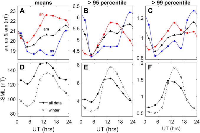
FIGURE 8. UT variations in (left column) mean values (middle column) the percentage of data exceeding the 95th-percentile; and (right column) the percentage of data exceeding the 99th-percentile for geomagnetic indices. The top row is for the mid-latitude am indices (Mayaud, 1980): the black line with black triangle symbols is for am, the red line with red circle symbols is for its northern hemisphere sub-index, an and the blue line with blue square symbols is for its southern hemisphere sub-index, as. The lower panel is for -SML, where SML is the SuperMAG auroral electrojet index, equivalent to AL and compiled from a large number (typically 100) of northern hemisphere stations (Newell and Gjerloev, 2011a; Newell and Gjerloev, 2011b). The solid line with filled circles is for all data and the dashed line with open circle symbols is for data taken within 15 days of the winter solstice. The am, an and as data are for 1959–2021, inclusive, and the SML data are 1976–2021, inclusive.

One such Index is the SuperMAG SML index (Newell and Gjerloev, 2011a; Newell and Gjerloev, 2011b). Like the AL index on which it is based (Davis and Sugiura, 1966), SML becomes increasingly negative with increased geomagnetic activity. Hence to avoid convoluted wording and potential confusion, we here use (−SML) in plots and descriptions. SML avoids some of the latitudinal and longitudinal (i.e., UT) limitations of AL by using a great many stations (typically 100) rather than just 12. It is available at 1-min resolution but, unlike am, it has the major limitation of being northern hemisphere only. There have been attempts to make the equivalent of the northern hemisphere AL index for the southern hemisphere, but the large expanses of ocean under long segments of the southern auroral oval mean that they show spurious UT variations (Maclennan et al., 1991; Weygand et al., 2014). Parts D–F of Figure 8 suggest some similarity to the UT behaviours of -SML and an, but we have no southern hemisphere equivalent to SML to test and see if it behaves like as. However, in parts D–F of Figure 8, we also plot the results for within 15 days of the winter solstice: the values are lower but show the same UT variation even though the EUV enhanced conductivity remains very small at these times, indicating conductivity enhancement by solar EUV is not the major factor causing the observed UT variations in the distribution of SML values.

The effect of the IMF ${[B_Y]}_{\mathit{GSEQ}}$ polarity on the magnetopause reconnection voltage Φ_D shown in Figure 7 shows that we need to evaluate the effect of this IMF polarity on the geomagnetic indices. This is done in Figure 9. The left-hand column is for ${[B_Y]}_{\mathit{GSEQ}}>0$, the middle column for ${[B_Y]}_{\mathit{GSEQ}}<0$ and the right-hand column for all data. As for Figures 7A, B, samples with ${[B_Y]}_{\mathit{GSEQ}}$ between plus and minus one standard error in the mean have been omitted. The predicted variations in Φ_D are plotted in the upper row. The solid line and solid circles show the mean values (averaged over all F) and the dashed line and open circles are the modes of the distribution of hourly means for that UT and IMF ${[B_Y]}_{\mathit{GSEQ}}$ classification. The second row is for -SML. Comparison of parts D and E show that the variations in -SML are quite different for the two ${[B_Y]}_{\mathit{GSEQ}}$ polarities, with the peak being lower and 6h later, relative to the preceding Φ_D peak, in E compared to D. Hence in both amplitude and phase relative to the Φ_D forcing, the variation is quite different for the two IMF ${[B_Y]}_{\mathit{GSEQ}}$ polarities. The two IMF polarities occur with almost equal probability distributions and this means there is a net UT variation for all -SML data, as shown in Figure 9F, unlike for Φ_D (see Figure 9C). The third row is the same for the am indices. For ${[B_Y]}_{\mathit{GSEQ}}>0$ (Figure 9G), the an peak is 2 h after the peak in -SML whereas the southern hemisphere index as peak is 1 h before that in -SML and considerably smaller than that in an. For ${[B_Y]}_{\mathit{GSEQ}}<0$ (Figure 9H) the peaks in an and as are 4.5 h and 5.5 h after the peak in -SML and, although the peak in as is the larger, it is larger by a far smaller factor than that by which an exceeds as in the ${[B_Y]}_{\mathit{GSEQ}}>0$ case.

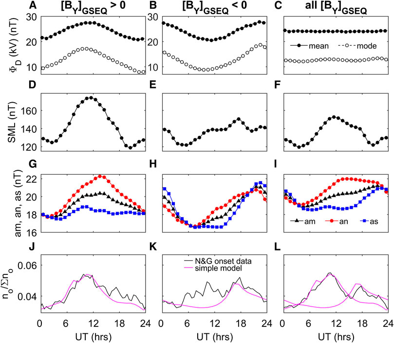
FIGURE 9. UT variations (averaged over all times of year F) of: (top row) the mean (black solid lines and black filled circles) and mode (black dashed line open circles) of the distribution of estimated magnetopause reconnection voltages, Φ_D, for the UT and IMF ${[B_Y]}_{\mathit{GSEQ}}$ polarity in question; (second row) the -SML index; (third row) the am, an and as indices (interpolated linearly from three-hourly values) (shown using the same symbols and colors as in Figure 8); and (bottom row) the normalised number of substorm onsets derived from the SuperMAG SML index using the algorithm of Newell and Gjerloev (2011a); Newell and Gjerloev (2011b) (black lines) with the predicted variations by a simple model described in the text (mauve lines). The left-hand column is for ${[B_Y]}_{\mathit{GSEQ}}>0$, the middle column for ${[B_Y]}_{\mathit{GSEQ}}<0$ and the right hand column for all ${[B_Y]}_{\mathit{GSEQ}}$. The data are for 1980–2021, inclusive, for which we have higher availability of IMF data.

Hence there is little symmetry in the response of these geomagnetic indices between the two IMF polarity cases. The bottom row of Figure 9 relates to substorm onset occurrence and is discussed later.

The asymmetry between the results for the two polarities of IMF ${[B_Y]}_{\mathit{GSEQ}}$ is analysed using the SML index in Figure 10, using the same format as Figure 7. The upper panel shows the F-UT patterns for -SML and the resulting UT variations (integrated over all F) are shown in the right-hand column. The contours of the IMF orientation factor in Φ_D from Figure 7 (for the simplified demonstration of the R-M effect with${[B_Z]}_{\mathit{GSEQ}}=0$) are re-plotted on the F-UT plots. In the lower panel the same format is used to plot the difference ΔSML = (−SML) − (−SML_p) where SML_p is a linear fit in the 1-min data of SML to Φ_D, averaged over the prior hour:

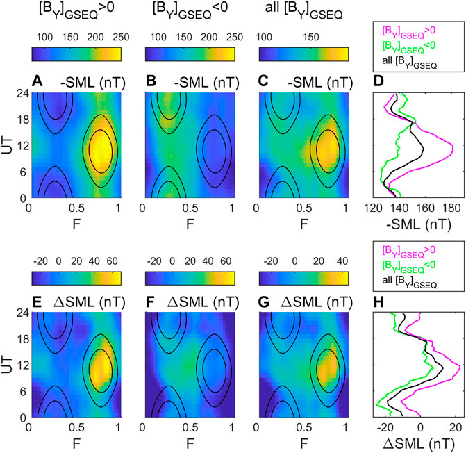
FIGURE 10. F-UT plots of the -SML index. Parts (A–D) show the means of −SML, parts (E–H) show means of ΔSML = SML_p − SML, where SML_p is computed from Φ_D using the linear fit given by Eq. 1. The two contours on each F-UT plot are as shown in Figure 7 and define the R-M peaks in the IMF orientation factor in Φ_D, sin^2.5(θ/2). From right to left the first column is for ${[B_Y]}_{\mathit{GSEQ}}>0$, the second for ${[B_Y]}_{\mathit{GSEQ}}<0$ and the third for all ${[B_Y]}_{\mathit{GSEQ}}$. The right-hand plots (D,H) show the averages of the index over all F as a function of UT: the green line is for ${[B_Y]}_{\mathit{GSEQ}}>0$, the mauve line for ${[B_Y]}_{\mathit{GSEQ}}<0$ and the black line for all ${[B_Y]}_{\mathit{GSEQ}}$. Data are for 1980–2021, inclusive.

Although −SML_p captures the trend of increasing −SML with increased Φ_D, there is considerable scatter between 1-min values of SML_p and SML: the r.m.s. difference between the two is 134 nT. Higher-order polynomials do not give a significantly lower r.m.s. fit residual (for example it is 133.6 nT for a second-order polynomial) and tests showed that all subsequent results were essentially independent of the polynomial order employed. Figure 10 investigates the origin of this scatter. Note that ΔSML quantifies the deviation from the expected SML for a linear dependence on the prevailing Φ_D, and hence from the R-M effect; Figure 10A shows that for ${[B_Y]}_{\mathit{GSEQ}}>0$ the major peak in Φ_D around 10UT in September, caused by the R-M effect, is accompanied by a major peak in SML. On the other hand; Figure 10B for shows that for ${[B_Y]}_{\mathit{GSEQ}}<0$, the corresponding peak in Φ_D at 22UT in March is accompanied by only a weak peak in SML and instead there is weak enhancement at almost all UT in March. The bottom panel shows the deviation from the expectations of the R-M effect, ΔSML. The main thing to note is that ΔSML is enhanced at all F between about 7 h UT and 18 h UT. This is even true for the solstices as well as the equinoxes. This UT variation is close to being in phase with the R-M variation for ${[B_Y]}_{\mathit{GSEQ}}>0$ and enhances the R-M variation around the September equinox peak but is in close to antiphase with the R-M variation for ${[B_Y]}_{\mathit{GSEQ}}<0$ and so reduces the amplitude of the R-M variation around the March peak. In addition to this strong variation with UT that is independent of F, parts E–G of Figure 10 reveal ΔSML shows a weaker, background equinoctial pattern.

The one other pair of indices that we have that are comparable in the two hemispheres are the polar cap indices, PCN and PCS (Troshichev et al., 2006), which are analysed in Figure 11. For both hemispheres, we use the definitive data of the IAGA-endorsed version of the indices, available for 1998–2020, inclusive (IAGA is the International Association of Geomagnetism and Aeronomy, one of the eight associations of the International Union of Geodesy and Geophysics). These indices are derived from enhancements of the horizontal H and D magnetic field components relative to the quiet level at two polar cap stations (Thule and Vostok, respectively, for PCN and PCS). The quiet level varies with UT and F because of ionospheric conductivity variations. For the original version of these indices, PCN was produced in Danish Meteoropogical Institute (DMI) and PCN by the Antarctic Research Institute (AARI) and the procedure used was not the same in the two cases. (McCreadie and Menvielle, 2010; Stauning, 2013). Hence, although the two were highly correlated, PCN was systematically 35% smaller than PCS and the difference grows when values are high (Lukianova et al., 2002; Ridley and Kihn, 2004). Since then, a “unified method” of processing has been developed at AARI (Troshichev et al., 2006; Troshichev, 2022) and in 2013 was approved by IAGA, as a new international index of the polar cap magnetic activity. All the IAGA-endorsed definitive data have been re-generated by this unified method, a task that was completed in 2021 and various anomalies resolved. There has been debate in the literature about outstanding anomalies (Stauning, 2022; Troshichev et al., 2022) but our investigations show that the currently-available definitive data give considerably greater agreement between PCS and PCN than used to be the case before application of the unified method, to the extent that remaining differences between PCS and PCN may well be real and it is the expectation that they should be the same that may be in error (For example, lobe stirring reconnection usually influences one polar cap but not the other).

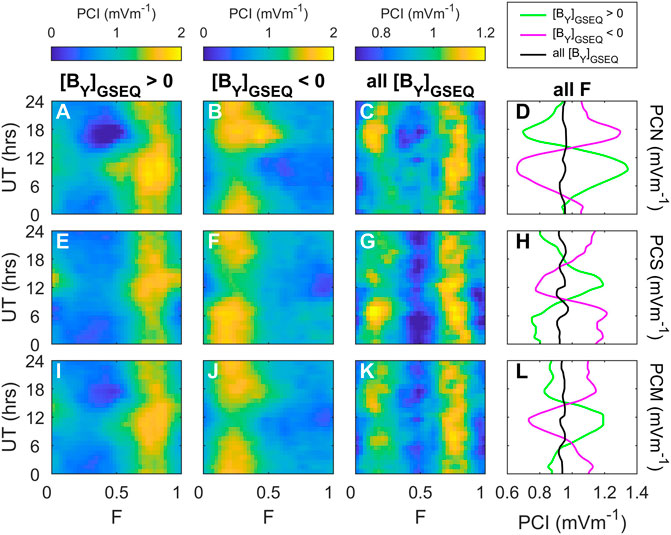
FIGURE 11. Definitive, IAGA-endorsed Polar Cap Index (PCI) data for 1998–2020, inclusive. The top row is for the Northern polar cap index, PCN, the middle row is for the Southern polar cap index, PCS, and the bottom row is for the average of the two (labelled, PCM: “M″ for “Mondiale” (global) to match the am index terminology). The first three columns (left to right) show F-UT, plots. The first is for ${[B_Y]}_{\mathit{GSEQ}}>0$, the second for ${[B_Y]}_{\mathit{GSEQ}}<0$ and the third for all ${[B_Y]}_{\mathit{GSEQ}}$. The right hand plots shown the averages of the index over all F as a function of UT: the green line is for ${[B_Y]}_{\mathit{GSEQ}}>0$, the mauve line for ${[B_Y]}_{\mathit{GSEQ}}<0$ and the black line for all ${[B_Y]}_{\mathit{GSEQ}}$.

The Polar Cap indices were originally proposed as approximate measures of the geoeffective interplanetary electric field. Induction effects mean that this can only be true with considerable averaging and not for the 1-min resolution with which the indices are generated. Comparisons with assimilative mapping of convection patterns from many data sources suggests PCN and PCS correlate best with reconnection voltage Φ_D rather than electric field. In fact, they appear to correlate least well with the polar cap electric field and there are also seasonally-varying differences (Ridley and Kihn, 2004).

Figure 11 shows the F-UT patterns for the PCI indices. Comparison with Figure 7 clearly reveals the R-M effect in both hemispheres when the data are sorted by the mean value (over the prior 10 min) of the IMF ${[B_Y]}_{\mathit{GSEQ}}$ component. However there is a notable tendency toward an equinoctial pattern to the equinox maxima for PCN but not PCS. The line plots in the right hand column of Figure 11 (UT variations averaged over all F) show that the UT variations for the two ${[B_Y]}_{\mathit{GSEQ}}$ components cancel almost perfectly leaving no UT variation in the combination for both ${[B_Y]}_{\mathit{GSEQ}}$ polarities. The PCI data primarily reflect the R-M solar wind to magnetosphere coupling mechanism. The slight hint of an equinoctial dipole tilt pattern in the northern hemisphere could have been in introduced by a slightly inaccurate allowance for conductivity effects or background subtraction in the analysis. Like the R-M effect, they do not show a net UT variation when data from both IMF ${[B_Y]}_{\mathit{GSEQ}}$ polarities are averaged together.

There is one more point to note about the polar cap indices. Although transformed into units of mVm⁻¹ they are essentially a magnetic field measurement and magnetic fields and currents (unlike electric field and flows) are the same in all reference frames. Hence although the observing magnetometers are moving back and forth in the X-direction with a diurnal variation, this does not influence the measurements, other than any effect the changing magnetospheric configuration and solar wind coupling has on the cross-cap current magnitude. This should be contrasted with ground-based radar data. These are measured in the frame of the radars that are moving in a geocentric-solar frame with the Earth’s rotation. Hence in a geocentric-solar frame the pole motion needs to be added to such data. Different again are satellite observations of electric fields and flows. These are measured in the satellite frame of reference and then transformed into a geocentric inertial frame using the knowledge of the motion of the satellite in that frame (Hairston and Heelis, 1993; Heelis and Hanson, 2013; Heelis et al., 2017). Hence satellite observations of convection flows and electric fields will include the effect of pole motions.

3 Universal Time variations in satellite observations of transpolar voltage

The PCI indices do not show any net UT variation. They have the advantage of being a continuous, homogeneous and long data series but are only an indirect measure of transpolar voltage. The problem with more direct observations, such as from satellites and radars, is that statistical surveys are dominated by sampling and aliasing effects. For example, even the 25-year survey of convection patterns from the SuperDARN radars by Lockwood and McWilliams (2021b) only yielded usable data for 30% of the time and the data gaps are not random but occur at certain seasons, UT and flow speeds. The problem when looking for an overall UT variation is that one is looking for the small difference betwen two large variations for the two IMF ${[B_Y]}_{\mathit{GSEQ}}$ polarities separately and, as illustrated by Figure 7, this leaves a small and noisy signal that is prone to distortion by the relative availability of data for the two IMF ${[B_Y]}_{\mathit{GSEQ}}$ polarities. Thus even this large SuperDARN data set is not suitable for detecting systematic UT variations. Satellite data give precise measurements along a given orbit but there are systematics in orbit occurrence that cause aliasing problems, meaning that, for example, a solar cycle variation can appear as a variation with F or UT.

A particular problem is that a Low-Earth Orbit (LEO) satellite measures the potential difference between two points but the orbit may not pass through, or even near, the maximum and minimum potentials on the polar cap boundary and so underestimate the true transpolar voltage. One method of dealing with this is to restrict surveys to passes that are close to along the dawn-dusk meridian that have most chance of sampling the full transpolar voltage (Doyle and Burke, 1983; Boyle et al., 1997). Alternatively statistical surveys, such as those by Weimer (2001) and by Lockwood et al. (2009) try to define the distribution of potential around the polar cap boundary and so can statistically correct the maximum and minimum potential seen in a given satellite pass to the maximum and minimum existing across the ionospheric polar cap.

Figures 12, 13 show F-UT plots of the DMSP F-13 and F-16 satellite data for 2001 and 2002, as processed by Lockwood et al. (2009). In both figures, the top row is for northern polar cap passes, the bottom for southern polar cap passes. Figures 12 and 13 are for intervals when the mean IMF ${[B_Y]}_{\mathit{GSEQ}}$ component, averaged over the hour prior to the pass, was positive and negative, respectively. The columns show (from left to right): the transpolar voltage, Φ_PC; the estimated polar cap flux F_PC; the simultaneous am index values; and the mean separation of the pass from the ideal 06–18 MLT meridian ⟨α⟩. The F and UT of each pass is defined by the time it is midway across the polar cap. Because the total number of passes is relatively low, a three-point running (boxcar) mean smoothing has been applied in these plots in both the F and UT dimensions. The open flux, F_PC, plots show a clear R-M pattern, like that seen in PCN and PCS. Comparison of the am plots (for only simultaneous data) with those presented by Lockwood et al. (2020b) and Lockwood et al. (2020a) for the full am dataset reveals the limitations of the smaller dataset.

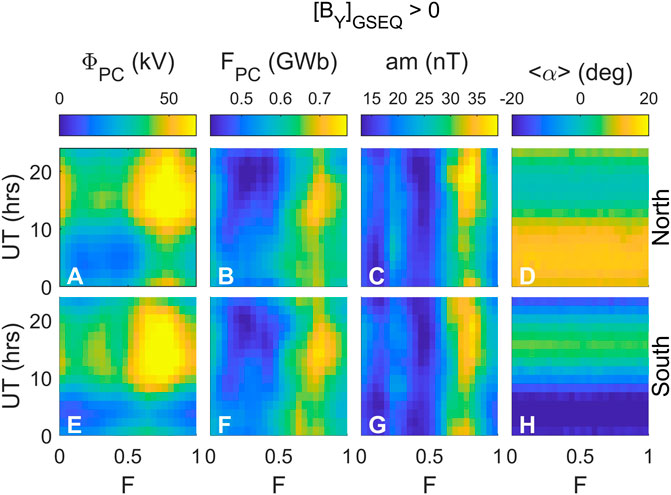
FIGURE 12. F-UT plots of the DMSP F-13 and F-16 satellite data for 2001 and 2002, as processed by Lockwood et al. (2009). The top row is for northern polar cap passes, the bottom for southern polar cap passes. These data are for intervals when the mean IMF ${[B_Y]}_{\mathit{GSEQ}}$ component, averaged over the hour prior to the pass, was positive. Mean values are shown in bins that are 1h wide in UT and (1/16)yr wide in F. Parts (A) and (E) are for the transpolar voltage, Φ_PC; parts (B) and (F) are for the estimate polar cap magnetic flux, F_PC; (C) and (G) are for the am index, linearly interpolated from the three-hourly data to the time of the mid-point of the polar cap traversal. (D) and (H) are for the mean separation of the pass from the ideal 06–18 MLT meridian ⟨α⟩, where α is the mean of the latitudinal deviations from the dawn-dusk meridian of the points of maximum and minimum potential along the orbit track. Because of the relatively short data series, 3-point running-mean smooths have been applied in both the F and UT dimensions.

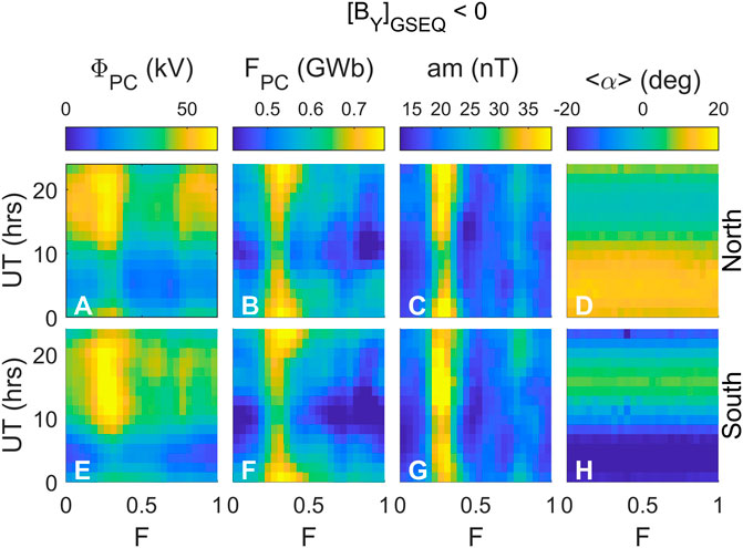
FIGURE 13. Same as Figure 12 for negative mean IMF ${[B_Y]}_{\mathit{GSEQ}}$.

The Φ_PC plots all show the dependence of the annual variation on IMF ${[B_Y]}_{\mathit{GSEQ}}$ that is predicted by the R-M effect with pronounced maxima at the relevant equinox. The mean values for the two hemispheres at equinox are always very similar as are the summer and winter solstice minima between the equinox peaks (see Figure 3 of Lockwood et al. (2020a)). However, Figures 12, 13 also show a large and regular UT variation with a pronounced minimum at about 1–9 h UT in both hemispheres. These minima appear not to be physical because the average values of Φ_PC fall as low as 17 kV which is lower than the average magnetopause reconnection voltage Φ_D predicted at the time, which is approximately 25 kV.

Parts D and H of Figures 12, 13 point to an important limitation of these data that is relevant to the apparent minimum in Φ_PC at 1–9 h UT. The parameter ⟨α⟩ is the mean of the latitudinal deviations from the dawn-dusk meridian of the points of maximum and minimum potential along the orbit track. Although the number of samples is high in each F-UT bin, some satellite passes were more removed from the ideal dawn-dusk meridian path than others. These panels show that for both IMF ${[B_Y]}_{\mathit{GSEQ}}$ polarities, near ideal passes (with |⟨α⟩| lower than about 5°) are seen in both hemispheres at about 12–23 h UT (colored green/light blue) but that in the Northern hemisphere at 01–09 h UT, ⟨α⟩ values are closer to +20° in the northern hemisphere (in orange), i.e., on the nightside of the 06–18 MLT meridian and to −20° in the southern hemisphere (in dark blue), i.e., on the dayside of the 06–18 MLT meridian. Hence the orbit characteristics are aliasing the UT variation with one in |⟨α⟩|. This sort of aliasing of variations frequently occurs in satellite data.

The point is that the analysis of Lockwood et al. (2009) extrapolates the observed voltage along the satellite path to the 06–18 MLT meridian using a statistical model of potential around the polar cap boundary and this extrapolation is most uncertain when |⟨α⟩| is large. We therefore treat the minimum at 01–09 h UT with suspicion as it was likely caused by, or at least enhanced by, sampling effects of the orbit configuration. As a result, in Figure 14 we study ΔΦ_PC, the deviation of mean Φ_PC for a given data subset (North or South and for positive or negative IMF ${[B_Y]}_{\mathit{GSEQ}}$) from the overall mean value at that UT to reduce any spurious UT variation caused by this aliasing.

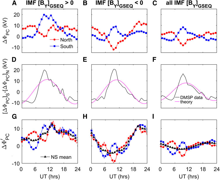
FIGURE 14. UT variations (averaged over all times of year F) of (top row) difference in mean transpolar voltages for the data subset in question and the overall mean value at that UT ΔΦ_PC; red line with circle symbols are for the northern hemisphere transpolar voltage, ${[\mathrm{\Delta }{\mathrm{\Phi }}_{PC}]}_N$, blue lines with square symbols for the southern, ${[\mathrm{\Delta }{\mathrm{\Phi }}_{PC}]}_S$. The data are the same DMSP observations for 2001 and 2002 as in Figures 12, 13. (middle row) The difference between the southern and northern polar cap voltages, ${[{\mathrm{\Phi }}_{PC}]}_S-{[{\mathrm{\Phi }}_{PC}]}_N$ (in black) and the predicted variation due to pole motions (in mauve). The effective polar cap diameters (f_c.d_PC) used to give best fit were: 1,390 km in (D); 1,300 km in (E); and 960 km in (F) (corresponding to latitudinal radii of 5.9°, 5.5°, and 4.1°), these giving the minimum r.m.s. deviation of the observed and model values) (bottom row). The ΔΦ_PC values after removal of the pole motion effect, $\mathrm{\Delta }{\mathrm{\Phi }}_{PC}^{\prime }=\mathrm{\Delta }{\mathrm{\Phi }}_{PC}+\varphi$. The left-hand column is for ${[B_Y]}_{\mathit{GSEQ}}>0$, the middle column for ${[B_Y]}_{\mathit{GSEQ}}<0$ and the right hand column for all ${[B_Y]}_{\mathit{GSEQ}}$.

Parts A–C of Figure 14 give clear evidence that the transpolar voltages are influenced by the pole motions. A Is for ${[B_Y]}_{\mathit{GSEQ}}>0$ during the pass and over the previous hour, B for ${[B_Y]}_{\mathit{GSEQ}}<0$ and C for all data. In all three cases the transpolar voltage is greater in the southern hemisphere between about 6.5 h UT and about 15.5 h UT when the southern/northern polar cap is moving anti-sunward/sunward, enhancing/reducing the transpolar voltage induced by the solar wind. At all UT before and after this interval the reverse applies. In order to scale the effect (for the unknown factor f_c. d_PC which is assumed constant) and allow for it, parts D–F of Figure 14 give the difference between the means of the Southern and the Northern transpolar voltages at a given UT ${[{\mathrm{\Phi }}_{PC}]}_S-{[{\mathrm{\Phi }}_{PC}]}_N$ (in black) and the model prediction for pole motions shown in Figure 5B (in mauve). These have been scaled to give the minimum r.m.s. difference between the observed and theoretical values and are for effective polar cap radii, f_c. d_PC, of 1390km, 1300km and 960 km in parts D–F, respectively. Parts G–I show the variations with the pole motions contributions removed $\mathrm{\Delta }{\mathrm{\Phi }}_{PC}^{\prime }=\mathrm{\Delta }{\mathrm{\Phi }}_{PC}-\varphi$, where ϕ is the relevant pole motion voltage, which is defined as positive when the polar cap is moving toward the Sun. ${\mathrm{\Phi }}_{PC}^{\prime }$ can be thought of as the voltage that would be seen if the pole was not moving in a geocentric-solar frame or as the voltage contribution induced by the solar wind flow.

It can be seen that removing the effect of the pole motions has made the $\mathrm{\Delta }{\mathrm{\Phi }}_{PC}^{\prime }$ values in the two hemispheres more similar at almost all UT. The important point about Figure 14 is that it shows the transpolar voltages are influenced by the pole motions in the way predicted in the introduction and by Lockwood et al. (2021), i.e., that when a given pole is moving sunward, the voltage across that polar cap in a geocentric-solar frame is reduced (and hence that the rate at which flux is added to the corresponding tail lobe is enhanced).

All three plots in the middle row of Figure 14 show the same deviations of the observed hemispheric difference (the black lines) from the expectation from pole motions (the mauve lines). This implies that the factor f_c. d_PC for each pole varies over the diurnal cycle in a regular way, rather than being constant, as has been assumed here. This therefore offers an potential explanation of why the results for the north and south hemisphere in the plots shown bottom row diverge somewhat at certain UTs in a similar way in all three cases.

4 Universal Time variations in substorm onset occurrence

Several lists of the times of substorm expansion phase onset (hereafter referred to as “onset”) have been compiled from different sources and covering different intervals. During expansion phases the following occur: brightening and expansion of the nightside aurora; dipolarization of the magnetic field in the near-Earth tail; injection of energetic particles into the inner magnetosphere; diversion of the cross-tail current into the ionosphere in the substorm current wedge (giving enhanced nightside auroral electrojet current and an increase in -SML); reduction of the magnetic flux and stored energy density in the magnetotail lobes; ULF wave activity seen in the ionosphere and magnetosphere. Onset can be defined by the first appearance of such phenomena, and from specific features such as the appearance of a westward travelling surge (or brightening of the pre-existing auroral arc), flow bursts in the mid-tail region and other signatures of enhanced tail reconnection, and a burst of Pi2 micropulsations (Kepko, 2004). The different lists of onset times vary considerably depending on the source of the data and are strongly influenced by the threshold adopted for the amplitude of the subsequent expansion phase (Forsyth et al., 2015). We here use the onset lists by Forsyth et al. (2015) (hereafter FEA) and by Newell and Gjerloev (2011a) and Newell and Gjerloev (2011b) (hereafter NG), both generated using the SML dataset. These lists have a higher number of onsets in an given interval than others and so include onsets of smaller substorms than other lists. It must be remembered that the SML index is compiled from northern hemisphere only data and this may have influenced the lists: however, expansion phase mechanisms such as enhanced tail reconnection, dipolarisation, and cross-tail current disruption necessarily involve both hemispheres and so there would be great similarities between the list for SML and that from a southern-hemisphere equivalent, particularly for the larger substorm expansion phases. However it is possible that some expansion phases would be small enough in one hemisphere to evade detection but not in the other. Thus we need to remember the possibility that these lists may omit some onsets that would only have been detectable in the Southern hemisphere.

Figure 15 compares the occurrence of onsets in these two lists: the upper row is for FEA and the lower one for NG. The total number in the interval 1976–2021 (inclusive) in the FEA list is Σn_FEA = 112,024 and that in the NG list is Σn_NG = 78,173: hence the FEA list contains 43% more onsets than that the NG list and the threshold criteria used in the FEA algorithm for defining a substorm expansion phase counted smaller expansions that the NG algorithm. The left-hand plots show the F-UT occurrence of onsets and the pattern is similar for the two lists. The plots are similar in many ways. Both show the equinoctial pattern but the UT variation along the equinoctial peaks is different for the two. For example, for the FEA onsets, 27.2% of onsets occur in the quarter of the year around the March equinox (F between 0.091 and 0.341) and 26.1% in the quarter around the September equinox (F between 0.603 and 0.853). Hence the number of onsets shows the semi-annual variation in that these numbers are elevated over the 25% for equal occurrence in all quarters, but not by as much as for most geomagnetic indices and the number of large storms. We sorted these data according to the polarity of the IMF ${[B_Y]}_{\mathit{GSEQ}}$ component during the growth phase (McPherron, 1972) prior to the onset (this was taken to be a 40 min interval prior to onset or the interval after the prior onset, whichever was the shorter). This showed that for ${[B_Y]}_{\mathit{GSEQ}}>0$, 29.6% were in the quarter around the September equinox and 23.6% around March. For ${[B_Y]}_{\mathit{GSEQ}}<0$, March was the dominant equinox with 30.3% of onsets in the quarter and 23.2% in the quarter around the September equinox. These trends were also all seen in the NG onset list and were slightly more clear, which is not surprising as the NG list contains fewer onsets and so is for larger substorms (28.5%, 21.9%, and 33.0% were in the March equinox quarter for all, positive and negative ${[B_Y]}_{\mathit{GSEQ}}$, respectively whereas the corresponding numbers for the September equinox quarter were 27.5%, 33.2% and 22.5%). We note that an effect of IMF ${[B_Y]}_{\mathit{GSEQ}}$ on onset occurrence at the solstices was also reported by Ohma et al. (2021).

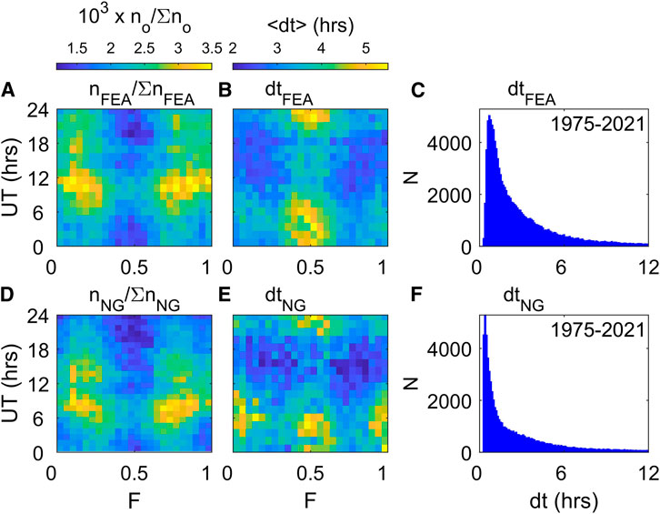
FIGURE 15. The occurrence of substorm onsets based on the SML geomagnetic index for 1976–2021, inclusive. The top row is for onsets identified by the SOPHIE algorithm of Forsyth et al. (2015) and the bottom row by the algorithm of Newell and Gjerloev, 2011a; Newell and Gjerloev, 2011b. The left-hand column are F-UT plots the numbers of onsets in bins of width 1 h in UT and 1/18 years in F, (A) being from the Forsyth et al. algorithm, n_FEA and (D) being for the Newell and Gjerloev algorithm n_NG. The middle column gives the corresponding F-UT plots of the mean time between onsets, dt_FEA in (B) and dt_NG in (E). The right hand panels give the overall distributions of these intervals between onsets.

Figures 15A, D show the F-UT occurrence of onsets for the FEA and NG lists, respectively. Both revealing that the semi-annual variation, noted above, has a distinct equinoctial form. However, these plots also show that the UT occurrence within that equinoctial form is certainly not uniform. For the FEA list there is a marked peak at 11–12 h UT for both the March and the September equinox and a second, weaker, peak roughly 6 h later, particularly for the March equinox. The same behaviour is seen for the NG list, but both peaks are roughly 1.5 h earlier than for the FEA list. Given that the FEA list contains more weak substorms, this indicates that the weaker substorms tend to have onset at a slightly later UT.

Parts B and D of Figure 15 show the same tendencies in a different way. They plot the F-UT pattern of mean duration of intervals between onsets (dt_FEA and dt_NG for the FEA and NG onset lists). Again an equinoctial pattern can be seen, but in the minimum values of dt. This is not just an equinoctial effect, the values of dt are larger at 0–7 h UT at all F. We note that this has some similarities to the conductivity F-UT pattern for both polar caps shown in Figure 6G, or that for both dayside auroral ovals in Figure 6H, but not seen in the corresponding plot for the nightside auroral oval in Figure 6I.

Figures 15C, E highlight that there are differences as well as similarities between the behaviour of onsets in the two lists by showing the distributions of dt_FEA and dt_NG, respectively. The two distributions have approximately the same form, but that for dt_FEA is noticeable broader. This means inter-onset intervals tend to be greater, even though more onsets are detected. The reason is that there are considerably more very short dt_NG values, showing that the NG list has more multiple-onset events that were classed as a single onset by the FEA algorithm.

We have constructed a simple Monte-Carlo numerical model of substorm growth phases that can explain the peaks of onset occurrence at around 11 h UT. This model starts from the fact that the upstream solar wind and IMF in the GSEQ frame are not influenced by the phase of Earth’s rotation. The IMF in the GSM frame (and hence the magnetopause reconnection voltage) is, of course, dependent on the UT of its arrival at Earth because of the changing angle of rotation between the GSEQ and GSM frames. The only UT influence on the dayside reconnection voltage is via the R-M effect and depends on the IMF ${[B_Y]}_{\mathit{GSEQ}}$. Let us start with the simplest case of constant Φ_D to illustrate the principles. We can take the times at which growth phases are started by an IMF orientation change to be random in UT. We simulate a very large number of growth phases (0.5 million) starting them all from a nominal flux values at a UT selected by a random number generator. We then consider the accumulation of open flux in both polar caps at a rate of Φ_D − Φ_N: because we are considering the average behaviour of a great many growth phases, we want to use an average value for the voltage Φ_D. We here also use a low value of Φ_N = 3 kV in these growth phases for simplicity. An overall average value of Φ_D is 24kV, and that is used for the right-hand panels in Figure 16. However, as that contains some very large values (150 kV and greater) and we also want to consider lower, mode values because they occur most often. The problem here is that, as demonstrated by Figure 4, the mode value of the distribution of Φ_D depends on the timescale τ that is considered. The left-hand panels in Figure 16 use an example value 15kV, which is the mode of the distribution of Φ_D for an averaging timescale of τ = 2h (see Figure 4C). This is larger than the duration of most growth phases, which were found in the survey by Partamies et al. (2013) to last for a mean duration around 48min And a median around 31min. However, some growth phases can last 3 h or even longer (Li et al., 2013). Note that the smaller the value of τ, the smaller is the mode (most common) value of Φ_D. This growth of flux in a lobe is modulated in the two hemispheres by the effects of the pole motions in the way shown in Figure 5C and our model allows for this effect by modulating the rate of growth of flux in a lobe accordingly; Figures 16A, B show the resulting variation of lobe flux accumulation with UT. The dashed line is of slope Φ_D − Φ_N = 12 kV in Figure 16A, 21 kV in Figure 16B. The red and blue lines show the effect on the lobe flux accumulation of making allowance for the pole motion on the northern and southern lobe, respectively (i.e., they have slope Φ_D − Φ_N + ϕ_n and Φ_D − Φ_N + ϕ_s where ϕ_n and ϕ_s are the pole-motion voltages in the northern and southern polar caps and both depend on UT as shown in Figure 5). The black line is the variation effect for the average of the two.

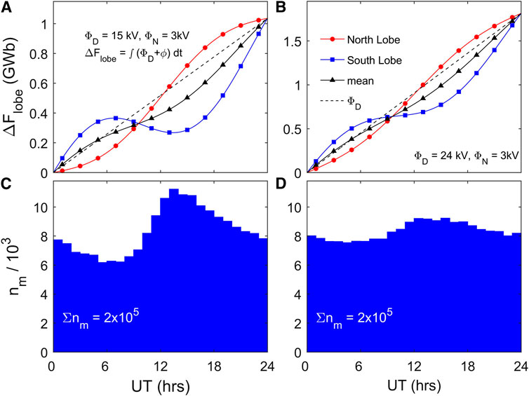
FIGURE 16. The results of a simple model of how the UT variation in substorm onset occurrence can be caused by the pole motion effect. The upper panels show the UT variations of magnetic flux accumulation in the tail lobes, ΔF = ∫(Φ_D − Φ_N + ϕ)dt: red (with red circle symbols) is for the northern hemisphere ΔF_N = ∫(Φ_D − Φ_N + ϕ_n)dt, blue (with blue square symbols) for the south ΔF_S = ∫(Φ_D − Φ_N + ϕ_s)dt and black (with black triangle symbols) is the mean of the two ΔF_M = (ΔF_N + ΔF_S)/2. In (A) Φ_D = 15 kV (the mode of the distribution for 2-h intervals) and Φ_N = 3 kV. In (B) Φ_D = 24 kV (the mean of the distribution) and Φ_N = 3 kV. Parts (C) and (D) show histograms of the numbers of onsets predicted by the simple model, n_m, as a function of UT. In the model, the onsets are triggered stocastically based on a probability that varies linearly with the mean lobe flux F_M = (F_N + F_S)/2 (See text for further details).

In the simple Monte-Carlo model, 0.5 million growth phases were started at a random UT from a baselevel tail flux given by ${[F_N]}_o={[F_S]}_o=$0.1 GWb (so the initial mean lobe flux, ${[F_M]}_o=$0.1 GWb). The question then arises when will the subsequent onset occur (and bring to an end each of the 0.5 million growth phases) and how do we predict this in the model? The triggering of substorm onsets has been discussed for many years and many mechanisms proposed (Spence, 1996; Lyons et al., 2018; Milan et al., 2019; Tanaka et al., 2021). Here we make use of the survey of open magnetospheric fluxes F_PC by Boakes et al. (2009) that does not define the precise time of onset but does give us a usable statistical relationship. These authors found that for values of F_PC below 0.3 GWb the probability of a substorm onset occurring was negligible but that as F_PC rose above this level the probability increased linearly and was undefined above 0.9 GWb. We take the flux in the tail lobe to be close to the polar cap flux F_PC (i.e., we neglect the open flux threading the dayside magnetopause). There will certainly be other factors, but to illustrate the concept we here take the probability of an onset occurring to increase linearly with the average lobe flux F_M from 0 at (and below) F_M = 0.3 GWb and reach unity at F_M = 1.2 GWb, which is postulated to be the largest value that F_PC can attain (Mishin and Karavaev, 2017). Note that lowering the assumed initial lobe flux value of 0.1 GWb increases the average length of the growth phases but does not influence the distribution of onset UTs because the start UT values are randomly chosen: the same is true for increased nightside tail reconnection voltage Φ_N that removes lobe flux. The value of F_M is recalculated every 1 s and onset determined to have occurred or not at each time step using a random number generator constrained to select onset occurrence based on the probability set by the F_M value. Hence this model of growth phase duration contains the influence of solar wind speed, IMF amplitude and orientation and preconditioning of the magnetosphere that are found to be key elements from machine learning (Maimaiti et al., 2019). The numbers of onsets simulated in different UT bins are shown in parts C and D of Figure 16. Part C demonstrates the key principles: at about 3–11 h UT the rate of accumulation of average (and hence total) tail flux dF_M/dt drops, because of the large antisunward motion of the South pole in the geocentric-solar frame. This means the rate at which growth phases reach an F_N value large enough to give a high probability of onset falls and the modelled number of onsets, n_m, falls. Subsequently the rate of growth in F_M recovers and above-average n_m values occur because growth phases that have been extended by the prior reduction in dF_M/dt reach onset. The same sequence occurs in part D but the larger value of Φ_D means that the effect of the polemotions is much less significant. Hence both the dip and the subsequent peak in onset occurrence is present in part D, but is much less pronounced.

It is possible to use this model to allow for the effect of an IMF ${[B_Y]}_{\mathit{GSEQ}}$ component by modulating the Φ_D value (either the mean or the mode) by the relevant variation with UT, as in top row in Figure 9. The results are shown by the mauve lines in Figures 9J, K for positive and negative ${[B_Y]}_{\mathit{GSEQ}}$, respectively. The rise/fall in Φ_D (depending on the IMF ${[B_Y]}_{\mathit{GSEQ}}$ polarity) causes the rate of increase in F_M over 0–12 h UT and this decreases/increases the size of the dip in n_m, making the feature seen in Figure 16C less/more pronounced and delaying/bringing forward the subsequent peak. Figures 9J, K also show the corresponding variation of observed onset numbers, n_o. These show that the variations do not separate into the positive and negative ${[B_Y]}_{\mathit{GSEQ}}$ cases as simply as the model and that, to some extent, both peaks in the UT variation are seen for both IMF ${[B_Y]}_{\mathit{GSEQ}}$ polarities. This is expected because the polarity of IMF ${[B_Y]}_{\mathit{GSEQ}}$ often flips in a growth phase and is consistent with the fact that the ${[B_Y]}_{\mathit{GSEQ}}$ polarities make only a partial separation of onsets into March or September.

This simple model shows us that pole motions can help to explain the unexpected UT variation observed onset numbers, n_o. The onsets agree well with the F-UT variations in -SML and am being at the time these indices start to increase. One feature of the model is that it predicts that it is substorms generated under weak solar wind forcing (low Φ_D) that give the UT variation in onset occurrence: this offers an explanation of why some onset lists show little or no UT variation if they are selected on substorms with large amplitude expansion phases.

5 Universal Time variations in field-aligned currents and ring current indices

The AMPERE project, described in the introduction, has yielded high resolution global mapping of the field-aligned currents (FACs) in both hemispheres for the years 2010–2016, inclusive. Coxon et al. (2016) showed that there is an almost sinusoidal diurnal dependence of total FAC intensities in one hemisphere (the sum of Region one and Region two and at all MLT) in good agreement with the effect of conductivity and a voltage source driving convection. We here sub-divide the AMPERE FAC data by R1 or R2 regions and by dawn or dusk. Figure 17 shows that there are regular UT variations in these currents when averaged over all years. In fact averages for each year individually show very similar patterns, but there are small differences from one year to the next that appear to depend on the phase of the solar cycle, but with only 7 years’ data it is too soon to say that definitively.

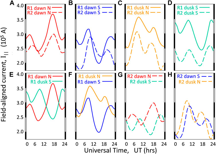
FIGURE 17. The UT variations of field-aligned currents in 6-h MLT windows around 06 and 18 h (dawn and dusk) defined by the AMPERE project from magnetometers on board the Iridium satellites. The upper panels compare the Region 1 (R1) currents (solid lines) and corresponding Region 2 (R2) currents (dashed lines). The lower panels compare currents in opposite hemispheres and opposite dawn-dusk sides of the magnetosphere using the same line types and colors as the upper panels. Data are for 2010–2016, inclusive.

The top panel of Figure 17 compares the latitudinally-integrated Region-1 (R1, solid lines) and Region-2 (R2, dashed lines) FACs in MLT ranges of 04:00–09:00 h (labelled dawn) and 14:00–21:00 h (labelled dusk). The plots are for dawn and dusk separately for both North and South hemisphere. The R1 and corresponding R2 have generally the same waveform and the R1 generally exceed the R2 as expected. However note there are times when this is not true and the R2 become comparable with the R1 or even exceed them. This happens at around 6 h UT for Northern hemisphere at dawn (Figure 17A) and, in particular, around 14 h UT for the Southern hemisphere at dawn (Figure 17B). These occurrences are interesting as they imply that the dawn auroral zone convection may have fallen to zero and even reversed to be antisunward. All the variations show a semi-diurnal variation, possibly implying that at least two mechanisms are at work. The intervals between the two peaks and between the two troughs is often around 12 h but rarely exactly 12 h, several being between 1 and 2 h different from that number.

The bottom row compares some combinations that show surprising correlations or anticorrelations. For example, the dawn R1 in the northern hemisphere are almost perfectly anticorrelated with the dusk R1 in the southern hemisphere (Figure 17E). This implies there is some net inter-hemispheric current flow as well as between dawn and dusk. It also implicates the UT variations in the ring current (that connects to the R2 FACs) that have reported in large ring current storms by Balan et al. (2021). An anticorrelation is seen for the converse combination (Northern dusk R1 and Southern dawn R1; Figure 17F) but is not as strong. The behaviour of the R2 currents is even stranger as the R2 currents in (Figure 17G) show a similar anticorrelation as the corresponding R1, yet the R2 currents corresponding to Figure 17F show a very strong correlation with a lag of about 2 h, as seen in Figure 17H. It is possible to devise many scenarios and causes for these relationships between the FACs but identifying definitively the causes is almost certainly going to require the use of a global MHD model of the coupled magnetosphere-ionosphere system with an eccentric dipole field model. Of relevance here are the findings of Mishin et al. (2021) who analysed FACs derived from magnetogram inversion techniques and of Coxon et al. (2016) from AMPERE results. These authors shown that R1 FAC intensities in the summer hemisphere exceed those in the winter hemisphere, indicating a conductivity effect that also induces a UT variation; Coxon et al. (2016) find an almost sinusoidal diurnal dependence of total FAC intensities in one hemisphere (R1 and R2 and dawn and dusk) whereas we see more complex semi-diurnal variations when we divide the data by R1 or R2 regions and by dawn or dusk. Coxon et al. (2016) also conclude that the total FAC current intensities are set by a combination of the magnetic flux throughput in the ECPC model and the polar conductivities. Mishin et al. (2021) report the sense of the inequality between FAC intensities in the dawn and dusk sectors was also shown to be different in the Northern and Southern Hemispheres which Mishin et al. (2021) attribute to an IMF ${[B_Y]}_{\mathit{GSEQ}}$ effect. This dawn-dusk asymmetry decreased with increasing substorm activity and almost completely disappeared in the winter hemisphere.

As mentioned above, the UT variations in the R2 FACs imply such osciallations should be seen in the ring current indices. We here use the four MLT-sector SMR partial ring current indices devised by Newell and Gjerloev (2012), SMR00, SMR06, SMR12, and SMR18 for the MLT quadrants around, respectively, midnight, dawn, noon and dusk. As for SML, these are increasingly negative for increased magnetic activity and so we plot and discuss the negative values. Figure 18 plots the UT variations in their mean values, separated into the two polarities of the mean IMF ${[B_Y]}_{\mathit{GSEQ}}$ over the previous hour.

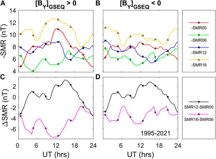
FIGURE 18. UT variations of the SuperMAG partial ring current indices, described by Newell and Gjerloev (2012). The top panels show -SMR00 (around midnight, in red with circle symbols); -SMR06 (around dawn, in green, with diamond symbols); -SMR12 (around noon, in blue with square symbols), and -SMR18 (around dusk, in orange with triangle symbols). The lower panels show the difference between the noon and midnight indices (SMR12-SMR00, in black with inverted triangle symbols) and between dawn and dusk indices (SMR18-SMR06, in mauve with star symbols). The left-hand column is for ${[B_Y]}_{\mathit{GSEQ}}>0$, and the right-hand column for ${[B_Y]}_{\mathit{GSEQ}}<0$. Data are for 1980–2021, inclusive.

The upper panels of Figure 18 shows that the midnight sector index -SMR00 (in red, with circle symbols) is enhanced around 12 h UT compared to the 00 h UT value. Both polarities show some enhancement just after 12 h UT, but this is much more pronounced for ${[B_Y]}_{\mathit{GSEQ}}>0$. On the other hand -SMR12 (in blue with square symbols) is similar for the two polarities with a persistent minimum at around 16 h UT. The -SMR18 index (in orange with triangle symbols) shows the clearest semi-diurnal variation that could relate to the FAC variations, with minima at 06 h UT and 20 h UT for both IMF ${[B_Y]}_{\mathit{GSEQ}}$ polarities. -SMR06 (in green with diamond symbols) has the smallest variation with elements of both a diurnal and a semi-diurnal variation. The bottom panel shows the differences between the dawn and dusk indices (in mauve with star symbols) and between noon and midnight (in black with inverted triangle symbols). Neither of these show a major difference in form with the IMF ${[B_Y]}_{\mathit{GSEQ}}$ polarity, but variations are somewhat smaller in amplitude for ${[B_Y]}_{\mathit{GSEQ}}<0$. It is expected that the difference SMR12-SMR00 would relate to the R2 FACs at dawn and dusk that connect to the ring current: hence it is not a surprise that this difference shows a marked semi-diurnal variation with two peaks and troughs. However this is superposed on a marked diurnal variation. Broadly speaking the semi-diurnal variations comes from the dayside SMR12 index whereas the diurnal comes mainly from the midnight SMR00 index.

A clue about the origin of these variations comes from studying the F-UT patterns of the means of the differences SMR12-SMR00 and SMR06-SMR18. These are shown in Figure 19. The top row shows the patterns for the midnight sector ring current SMR00 index. These show the semi-annual, variation with the equinox peaks, but with only a relatively small UT variation because of the long integration times of ring current forcing and the long loss timescales of ring current particles (Lockwood et al., 2016). Nevertheless there is a clear UT variation that is the same in Parts A–C with the equinoctial peaks being largest at 12–14 h UT and lowest at 23-01 h UT. However the middle row of Figure 19 shows that the difference in the noon and midnight partial ring currents, SMR12-SMR00, has considerable UT variation that does not vary greatly with time-of-year, F. This is a behaviour expected for phenomena induced by sunward-antisunward pole motions and so may indicate that this is the effect influencing the noon-midnight asymmetry of the ring current and hence the dawn and dusk FACs shown Figure 17. In contrast, the F-UT patterns for the difference SMR18-SMR06, shown in the bottom row of Figure 19 reveals a equinoctial dipole tilt pattern, suggesting an origin in conductivity effects and or tail dynamic effects. We note that Haaland and Gjerloev (2013) report a correlation between the dawn-dusk asymmetry in the partial ring currents is associated with a corresponding asymmetry in the magnetopause currents. This is another feature of the FAC/ring current/magnetopause current system that requires an explanation.

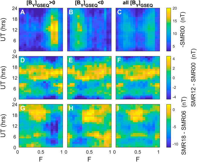
FIGURE 19. F-UT variations of selected SuperMAG partial ring current indices described by Newell and Gjerloev (2012). The top row is for -SMR00, the middle row for SMR12-SMR00 and the bottom row for SMR18-SMR06. The left-hand column is for ${[B_Y]}_{\mathit{GSEQ}}>0$, the middle column for ${[B_Y]}_{\mathit{GSEQ}}<0$ and the right-hand column for all ${[B_Y]}_{\mathit{GSEQ}}$. Data are for 1980–2021, inclusive.

6 Reconnection voltage variations and polar cap expansion and contraction

Lastly we look at the implications for UT variations in the magnetopause and cross-tail reconnection voltages (Φ_D and Φ_N, respectively) and the expansion and contraction of the polar cap. To do this we need to look for any UT variation in the polar cap flux. We use two sources of information on this, shown in the top row of Figure 20. The green lines show the polar cap flux F_PC derived from the AMPERE data for 2010–2016 using the technique described by Milan et al. (2021). The red and blue lines are from the DMSP data for 2001–2002 that we used earlier. The algorithm used by Lockwood et al. (2009) to compute F_PC gives values that are systematically higher than those derived in subsequent studies. In particular, the latitudinal gap between the convection reversal boundary (CRB) and the open-closed field-line boundary (OCB) was underestimated by Lockwood et al. (2009) and in this paper, revised estimate are employed made using a 4° separation between the CRB and the OCB, the same as used by Milan et al. (2021) between the poleward edge of the R1 currents and the OCB. The results agree quite closely with the AMPERE results. We here use the UT variations in F_PC from the DMSP data, averaging the (very similar) estimates from the North and the South polar caps: results were very similar, but a little noisier, if we used the AMPERE results.

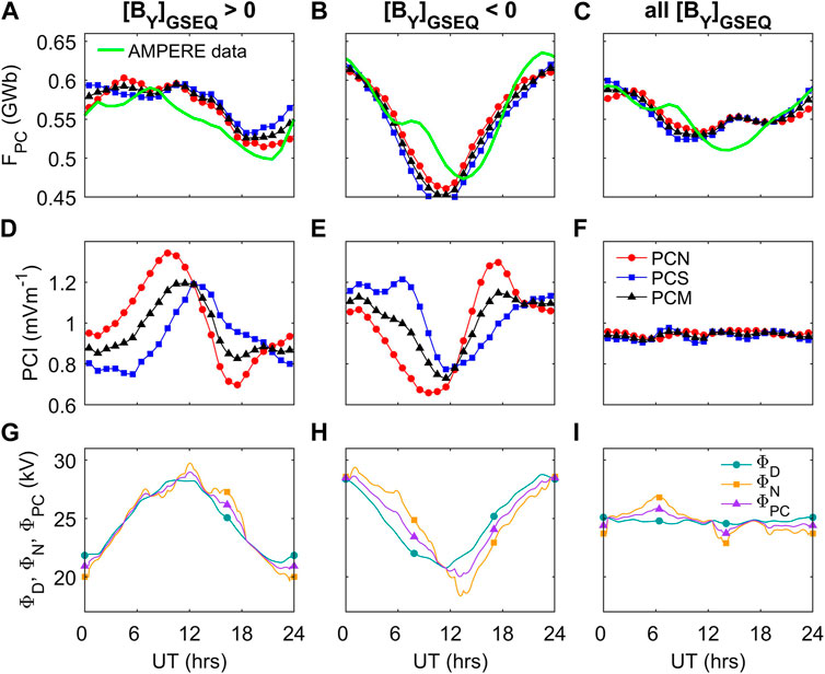
FIGURE 20. Analysis of UT variations in reconnection rates and the expansion and contraction of the polar cap. The top row shows the estimated variations of the polar cap flux F_PS from the AMPERE field-aligned current data (in green), and from the DMSP convection data for the Northern hemisphere (in red with circle symbols) and the Southern hemisphere (in blue with square symbols). The model shows the Polar Cap Index variations presented in the right hand column of Figure 11, but this time comparing PCN, PCS and PCM for one IMF ${[B_Y]}_{\mathit{GSEQ}}$ classification. The bottom row shows the variations in the estimations of magnetopause reconnection voltage Φ_D (green with circle symbols), cross tail current sheet voltage Φ_N (orange with square circles) and the transpolar voltage Φ_PC (mauve with triangle symbols). The left-hand column is for ${[B_Y]}_{\mathit{GSEQ}}>0$, the middle column for ${[B_Y]}_{\mathit{GSEQ}}<0$ and the right-hand column for all ${[B_Y]}_{\mathit{GSEQ}}$.

We differentiate F_PC and, applying Faraday’s law in integral form to the OCB (equivalent to continuity of open flux), we equate this to the voltage difference (Φ_D − Φ_N). Using the predicted UT variation in Φ_D from IMF data, this gives us the corresponding variation in Φ_N. We also compute the transpolar voltage for the assumption that the polar cap remains circular and neglecting any viscous-like interaction voltage (Lockwood, 1993; Milan, 2004). The results are shown in the bottom row of Figure 20. The middle row shows the Polar Cap Index variations, as also shown in the right hand column of Figure 11, but this time comparing the UT variations in the north, south and global indices (i.e., PCN, PCS and PCM) for one IMF ${[B_Y]}_{\mathit{GSEQ}}$ classification. As in previous figures, the left hand column is for ${[B_Y]}_{\mathit{GSEQ}}>0$, the middle column for ${[B_Y]}_{\mathit{GSEQ}}<0$ and the right hand column for all ${[B_Y]}_{\mathit{GSEQ}}$.

Figure 20 shows that for IMF ${[B_Y]}_{\mathit{GSEQ}}>0$, on average, Φ_N rises with the rise in Φ_D over 02–12 h UT caused by the R-M effect, such that F_PC remains approximately constant. This appears to be “driven” reconnection in which the slow increase in Φ_D means that Φ_N is always responding. However, we need to remember that this is average behaviour and not a single time series. There are short times toward the end of this interval when Φ_N exceeds Φ_D in what looks like substorm activity bursts at the times just after when onsets become more common. The third of these intervals is when Φ_D has begun to fall again and the polar cap contracts. Between 22 h UT and 02 h UT Φ_D exceeds Φ_N and the polar cap expands again to complete the average diurnal cycle.

This cycle is quite different for IMF ${[B_Y]}_{\mathit{GSEQ}}<0$. In this case the minimum of the open flux is near 12UT after which the R-M effect causes Φ_D to rise. Unlike the corresponding interval of rise for ${[B_Y]}_{\mathit{GSEQ}}>0$, Φ_N never matches ${\mathrm{\Phi }}_D$ and the polar cap expands considerably to peak at around 00 h UT when the R-M effect causes Φ_D to fall but, as for the rise, Φ_N only responds after a lag and the polar cap shrinks again.

When we average these two diurnal cycles together we see a net variation with a slight decrease in polar cap flux before about 12 h UT, followed by a very slight rise in the remainder of the diurnal cycle.

We note that the UT variations on the transpolar voltage Φ_PC inferred here in the bottom row of Figure 20 for the two polarities of IMF ${[B_Y]}_{\mathit{GSEQ}}$ mirror those seen in ΔΦ_PC from the DMSP data (which is an estimate of Φ_PC obtained by removing the effect in the observations of the systematic variation in the satellite orbit paths) shown in the bottom row of Figure 14.

7 Discussion and conclusion

We are aware that this comprehensive survey of average UT variations observed in the magnetosphere has raised considerably more questions than it has answered.

One thing that is clear is that the magnetospheric response during one polarity of the IMF B_Y component (in the GSEQ frame) is not cancelled out by that during the other polarity. This apparently does not arise from the solar wind forcing. The Russell-McPherron effect (Russell and McPherron, 1973) predicts that which equinox shows enhanced activity depends on that polarity and the UT variation is shifted by 12 h. The Polar Cap Indices confirm that this is largely the case. Hence it is clear that the response of the magnetosphere depends on UT such that the response for the two IMF ${[B_Y]}_{\mathit{GSEQ}}$ polarities is radically different. This implies there is at least one more inherent UT variation in the magnetosphere system. This was realised by Ruohoniemi and Greenwald (2005) who invoked the UT variation in ionospheric conductivity as the reason why changing ${[B_Y]}_{\mathit{GSEQ}}$ polarity does not simply induce a 12-h shift in the magnetospheric response as well as favouring the other equinox.

Ionospheric conductivity changes could indeed be all or part of the cause and have been invoked in the past more frequently than any other cause. However, in this review we have pointed out there are a number of other possibilities.

Both ${[B_Y]}_{\mathit{GSEQ}}$ polarities give a relative lull in the geomagnetic response between about 00 h and 10 h UT which ends with a period of higher occurrence of substorm onsets, enhanced auroral electrojet activity, followed by particle injections into the ring current and enhanced mid-latitude geomagnetic disturbance. The difference is that for ${[B_Y]}_{\mathit{GSEQ}}>0$ these responses are prompt whereas for ${[B_Y]}_{\mathit{GSEQ}}<0$ they are delayed, more gradual and of smaller amplitude. In terms of open flux continuity there is very little lag between the dayside and nightside reconnection rate changes for ${[B_Y]}_{\mathit{GSEQ}}>0$ whereas there is lag for ${[B_Y]}_{\mathit{GSEQ}}<0$ (and hence a larger diurnal cycle in the polar cap flux and size and a diurnal cycle of energy storage and release in the tail) which is almost entirely absent for ${[B_Y]}_{\mathit{GSEQ}}>0$. This is certainly is not to say that the 2–3h substorm cycles of storage and release are not present for both polarities, just that an underlying diurnal cycle is only present for ${[B_Y]}_{\mathit{GSEQ}}<0$.

We have presented an outline of a mechanism that can explain this - namely that the motions of the geomagnetic poles in a geocentric-solar frame reduce/enhance transpolar voltage in a diurnal cycle and thereby simultaneously increase/decrease the rate of energy storage in the corresponding tail lobe. Because of the eccentric nature of Earth’s dipole field these cycles are larger in the southern hemisphere and the northern and southern hemisphere cycles are not in perfect antiphase.

An alternate mechanism that can cause all of the above cycles arises from diurnal cycles in polar ionospheric conductivity due to photoionization by solar EUV and X-ray radiation. Enhanced conductivity can also reduce transpolar voltage and so increase the rate of energy storage in that tail lobe. In addition, as discussed in the introduction, other mechanisms have been proposed to yield the equinoctial pattern of activity including the effect of the tail hinge angle (and so the dipole tilt) on stability of the tail and the effect of dipole tilt on the accumulation of flux in the summer lobe.

How can we differentiate between these mechanisms? The first method is to study the F-UT patterns of observed features. The conductivity (in both hemispheres), tail bending and flux accumulation in the summer lobe mechanisms all yield an equinoctial pattern, that varies with both F and UT whereas the pole-motion effect gives the same UT variation at all F. Hence changes due to the latter give horizontal features in a plot with F along the horizontal axis and UT along the vertical axis (which is the convention adopted throughout this paper). However, a complication that must be folded in here is the R-M effect that gives the patterns shown in Figure 7 but which is only seen strongly when the data are sorted by the IMF ${[B_Y]}_{\mathit{GSEQ}}$ component. This gives variation with UT but that are 12 h out of phase for the two equinoxes.

In this paper, four related and important features were found to show F-UT patterns that were dominated by mainly horizontal structures in the F-UT patterns. The first is the deviation of the SML index from the expectation of the R-M mechanism (ΔSML) which has almost the same variation with UT at all F (see parts E–G of Figure 10). The second was the difference between the noon and midnight SMR partial ring current indices [(SMR12-SMR00), see parts D–F of Figure 19]. This difference in partial ring current indices is associated with particle injections in the midnight sector and hence substorm expansions. Hence it is also connected to substorm onset occurrence and the intervals between substorm onsets, which all show dominant horizontally-aligned features on an F-UT plot (Figure 19) which are predicted uniquely by pole-motion induction effects. We have also detected the pole motion effect in satellite transpolar voltage measurements. All of these consistent variations with UT are superposed on a weaker, background equinoctial pattern. Hence the F-UT patterns suggest a strong effect of pole motions on transpolar voltage and flux storage in the corresponding lobe, but with a secondary effect of conductivity changes or tail mechanisms that depend on the dipole tilt. We note that the same conclusion was reached by Lockwood et al. (2021) who used a mixture of pole-motion effects, conductivity changes, and dipole tilt effects on the tail to explain the UT variations and F-UT patterns of the mid-latitude am, an and as indices. It should be noted that an equinoctial pattern certainly does not identify a conductivity effect; indeed, Lockwood et al. (2020a) showed that the amplitude of the equinoctial pattern increased with increased solar wind dynamic pressure which strongly suggests that it originates in the dipole tilt effect on the geomagnetic tail.

The second comparison we can make looks at the timings of features. Figure 21 compares the expected UT variations for the two. The only difference in the waveform is slight in that the pole-motion effects are sinusoidal (part C), but because of the non-linearity of the conductivity effect on transpolar voltage, as illustrated by the results of Ridley et al. (2004) (shown in part A), the variations deviate from sinusoidal for conductivity (part D), particularly for the southern hemisphere at around 16UT when that polar cap is tipped away from the Sun and Σ_p is particularly low.

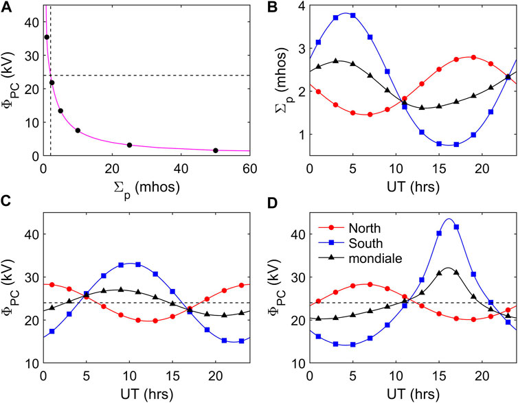
FIGURE 21. Comparison of the basic predictions of the pole motion and conductivity mechanisms. (A) Shows the dependence of transpolar voltage Φ_PC on the polar cap Pedersen conductivity Σ_p found from numerical simulations by Ridley et al. (2004) (their Figure 1B). (B) Shows the UT variations of the average polar cap Pedersen conductivity Σ_p from Figure 6). (C). The transpolar voltage for a daily mean of 24 kV caused by pole motions (from Figure 5B) and (D) the transpolar voltage change caused by the conductivity changes in part (B), scaled using the variation in part (A) to a daily mean of 24 kV as in (C). Red lines with red circle symbols are for the northern hemisphere, blue lines with blue square symbols for the southern hemisphere and black lines with black triangle symbols are the global (mondiale) values obtained by averaging the two.

However, the main difference we wish to explore here is the phase difference between the variations. Maximum decrease/increase in transpolar voltage due to pole motions is when the polar cap is moving faster toward/away from the Sun. On the other hand, maximum decrease/increase in transpolar voltage due to the conductivity effect is when Σ_p is a maximum/minimum which occurs when the polar cap is most inclined toward/away from the Sun. Hence the phase difference between the pole motion effects and the conductivity variation is π/4 (i.e., 6 h). Looking at the variations with UT presented here, most agree with the phase in Figure 21C and are inconsistent with the phase in Figure 21D. Hence, as from the UT-F patterns, we deduce the pole motion effect is dominant over the conductivity effect (but can find evidence that both occur).

This paper has concentrated on UT variations in mean values. These can be influenced by a few super-large events but generally reflect persistent but smaller changes at lower solar-terrestrial activity levels. This certainly seems to be the case in the substorm onset occurrence variation which we predict will not be present if one looks only at large events. Nevertheless, Figure 8 shows that the occurrence of large events in the -SML, am, an and as indices all follow the same form of UT variation as the mean values. Therefore the phenomena discussed here have relevance to the large-event tails of activity distributions as well as the mean values.

Some of the UT variations presented here are less easily explained although they are very likely to be rooted in those discussed above. This includes several of the partial ring current variations and the field-aligned current variations. Rather than postulate on their causes, we believe explanation will require runs from a global MHD numerical model of the magnetosphere-ionosphere system (which automatically maintains the key factor of current continuity) with a realistic lower boundary reproducing the Σ_p variations and an eccentric dipole magnetic field that influences both the conductivity and replicates inductive changes in the transpolar voltage and the rate of flux accumulation in the tail lobes. There seems to be no particular technical difficulty in employing an eccentric dipole in a global magnetosphere-ionosphere, but it is important to note experiments at a fixed tilt, whilst revealing some effects (such as those due to conductivity) will not show pole-motion induction effects. There will be a lot more effects if the themosphere is self-consistently coupled into the simulation due to the hemispheric difference in pole offsets (Cnossen et al., 2012; Förster and Cnossen, 2013; Laundal et al., 2017), the ionospheric behaviour being ordered relative to the geomagnetic pole and the neutral thermospheric behaviour ordered relative to the rotational pole.

There are also implications of the UT variations in the response to solar wind forcing for space weather forecasting. Lockwood et al. (2023) have estimated the effect of the UT of arrival of the CMEs that caused the storms in February 2022 that led to the loss of 38 out of 49 recently-launched Starlink Satellites. They found considerable effects on the division between directly-deposited energy and energy stored in the tail and released later. They also found effects on the distribution of energy deposited in the two hemispheres and its variation with event time. This strongly implies that it is important to forecast the precise time at which CMEs will impact the Earth and also to predict what this will mean for the evolution of the subsequent event in near-Earth space.

Author contributions

ML carried out the analysis of geomagnetic and transpolar observation data and SM carried out the analysis of the AMPERE field-aligned current data. ML wrote the text after discussions with SM who proof-read the paper.

Funding

ML was supported by consolidated grants number ST/R000921/1 and ST/V000497/1 from the United Kingdom Science and Technology Facilities Council (UKRI/STFC) and by the SWIGS Directed Highlight Topic Grant number NE/P016928/1/and grant NE/S010033/1 from the United Kingdom Natural Environment Research Council (UKRI/NERC). SEM was supported by STFC Grant No. ST/S000429/1.

Acknowledgments

The authors are grateful to the many instrument scientists and engineers who make the datasets employed in this study possible and the staff of a number of datacentres who allow easy access to the data. These include: the Space Physics Data Facility (SPDF) at NASA’s Goddard Space Flight Center for the Omni composite of interplanetary observations; the International Service of Geomagnetic Indices (ISGI), France and collaborating institutes for the am, PCN and PCS geomagnetic indices; the PIs and staff of the many groups contributing data to the SuperMAG project, coordinated at The Johns Hopkins University Applied Physics Laboratory, for the SMR and SML indices. Both authors are grateful the United Kingdom Science and Technology Facilities Council (UKRI/STFC) for grant support and ML also thanks the United Kingdom Natural Environment Research Council (UKRI/NERC) for additional support at the start of this project.

Conflict of interest

The authors declare that the research was conducted in the absence of any commercial or financial relationships that could be construed as a potential conflict of interest.

Publisher’s note

All claims expressed in this article are solely those of the authors and do not necessarily represent those of their affiliated organizations, or those of the publisher, the editors and the reviewers. Any product that may be evaluated in this article, or claim that may be made by its manufacturer, is not guaranteed or endorsed by the publisher.

References

Ahn, B.-H., Kroehl, H. W., Kamide, Y., and Kihn, E. A. (2000). Universal time variations of the auroral electrojet indices. J. Geophys. Res. Space Phys. 105, 267–275. doi:10.1029/1999JA900364
Ahn, B.-H., and Moon, G.-H. (2003). Seasonal and universal time variations of the AU, AL and Dst indices. J. Korean Astronomical Soc. 36, 93–99. doi:10.5303/JKAS.2003.36.SPC1.093
Alexeev, I. I., Belenkaya, E. S., Kalegaev, V. V., Feldstein, Y. I., and Grafe, A. (1996). Magnetic storms and magnetotail currents. J. Geophys. Res. Space Phys. 101, 7737–7747. doi:10.1029/95JA03509
Anderson, B. J., Korth, H., Waters, C. L., Green, D. L., Merkin, V. G., Barnes, R. J., et al. (2014). Development of large-scale birkeland currents determined from the active magnetosphere and planetary Electrodynamics response experiment. Geophys. Res. Lett. 41, 3017–3025. doi:10.1002/2014GL059941
Aoki, T. (1977). Influence of the dipole tilt angle on the development of auroral electrojets. J. geomagnetism Geoelectr. 29, 441–453. doi:10.5636/jgg.29.441
Atkinson, G. (1967). An approximate flow equation for geomagnetic flux tubes and its application to polar substorms. J. Geophys. Res. 72, 5373–5382. doi:10.1029/JZ072i021p05373
Atkinson, G. (1978). Energy flow and closure of current systems in the magnetosphere. J. Geophys. Res. 83, 1089–1103. doi:10.1029/JA083iA03p01089
Balan, N., Ram, S. T., Manu, V., Zhao, L., Xing, Z., and Zhang, Q. (2021). Diurnal UT variation of low latitude geomagnetic storms using six indices. J. Geophys. Res. Space Phys. 126. doi:10.1029/2020JA028854
Bartels, J. (1925). Eine universelle tagesperiode der erdmagnetischen. aktivität. Meteorol. Z. 42, 147–152.
Bartels, J. (1928). “Periodische variationen. aktivität,” in Handbuch der Experimentalphysik. Editors G. Angeneeister, and J. Bartels (Leipzig: Akademische Verlagsgesellschaft), 25, 624–665. chap. Das Magnetfeld der Erde.
Berthelier, A. (1990). Comment on “The universal time variatlon of magnetic activity”. Geophys. Res. Lett. 17, 307–308. doi:10.1029/GL017i003p00307
Berthelier, A. (1976). Influence of the polarity of the interplanetary magnetic field on the annual and the diurnal variations of magnetic activity. J. Geophys. Res. 81, 4546–4552. doi:10.1029/JA081i025p04546
Boakes, P. D., Milan, S. E., Abel, G. A., Freeman, M. P., Chisham, G., and Hubert, B. (2009). A statistical study of the open magnetic flux content of the magnetosphere at the time of substorm onset. Geophys. Res. Lett. 36, L04105. doi:10.1029/2008GL037059
Borovsky, J. E., Lavraud, B., and Kuznetsova, M. M. (2009). Polar cap potential saturation, dayside reconnection, and changes to the magnetosphere. J. Geophys. Res. Space Phys. 114. doi:10.1029/2009JA014058
Boyle, C. B., Reiff, P. H., and Hairston, M. R. (1997). Empirical polar cap potentials. J. Geophys. Res. Space Phys. 102, 111–125. doi:10.1029/96JA01742
Brambles, O. J., Lotko, W., Zhang, B., Oulette, J., Lyon, J., and Wiltberger, M. (2013). The effects of ionospheric outflow on ICME and SIR driven sawtooth events. J. Geophys. Res. Space Phys. 118, 6026–6041. doi:10.1002/jgra.50522
Brekke, A., and Moen, J. (1993). Observations of high latitude ionospheric conductances. J. Atmos. Terr. Phys. 55, 1493–1512. doi:10.1016/0021-9169(93)90126-J
Carter, J. A., Milan, S. E., Paxton, L. J., Anderson, B. J., and Gjerloev, J. (2020). Height-integrated ionospheric conductances parameterized by interplanetary magnetic field and substorm phase. J. Geophys. Res. Space Phys. 125. doi:10.1029/2020JA028121
Chapman, S., and Bartels, J. (1940). “Geomagnetism volume 1: Geomagnetic and related phenomena. No. 6,” in International series of monographs on Physics (London: Oxford University Press).
Chu, X., McPherron, R. L., Hsu, T., and Angelopoulos, V. (2015). Solar cycle dependence of substorm occurrence and duration: Implications for onset. J. Geophys. Res. Space Phys. 120, 2808–2818. doi:10.1002/2015JA021104
Cliver, E. W., Kamide, Y., and Ling, A. G. (2000). Mountains versus valleys: Semiannual variation of geomagnetic activity. J. Geophys. Res. Space Phys. 105, 2413–2424. doi:10.1029/1999JA900439
Cnossen, I., Wiltberger, M., and Ouellette, J. E. (2012). The effects of seasonal and diurnal variations in the Earth’s magnetic dipole orientation on solar wind-magnetosphere-ionosphere coupling. J. Geophys. Res. Space Phys. 117. doi:10.1029/2012JA017825
Cowley, S. W. H., and Lockwood, M. (1992). Excitation and decay of solar wind-driven flows in the magnetosphere-ionosphere system. Ann. Geophys. 10, 103–115. ADS Bibcode: 1992AnGeo.10.
Coxon, J. C., Milan, S. E., Carter, J. A., Clausen, L. B. N., Anderson, B. J., and Korth, H. (2016). Seasonal and diurnal variations in AMPERE observations of the Birkeland currents compared to modeled results. J. Geophys. Res. Space Phys. 121, 4027–4040. doi:10.1002/2015JA022050
Crooker, N. U., and Rich, F. J. (1993). Lobe cell convection as a summer phenomenon. J. Geophys. Res. Space Phys. 98, 13403–13407. doi:10.1029/93JA01037
Crooker, N. U., and Siscoe, G. L. (1986). On the limits of energy transfer through dayside merging. J. Geophys. Res. 91, 13393. doi:10.1029/JA091iA12p13393
Danilov, A. A., Krymskii, G. F., and Makarov, G. A. (2013). Geomagnetic activity as a reflection of processes in the magnetospheric tail: 1. The source of diurnal and semiannual variations in geomagnetic activity. Geomagnetism Aeronomy 53, 441–447. doi:10.1134/S0016793213040051
Davis, T. N., and Sugiura, M. (1966). Auroral electrojet activity index AE and its universal time variations. J. Geophys. Res. 71, 785–801. doi:10.1029/JZ071i003p00785
de La Sayette, P., and Berthelier, A. (1996). The am annual-diurnal variations 1959-1988: A 30-year evaluation. J. Geophys. Res. Space Phys. 101, 10653–10663. doi:10.1029/96JA00165
DeJong, A. D., Cai, X., Clauer, R. C., and Spann, J. F. (2007). Aurora and open magnetic flux during isolated substorms, sawteeth, and SMC events. Ann. Geophys. 25, 1865–1876. doi:10.5194/angeo-25-1865-2007
Doyle, M. A., and Burke, W. J. (1983). S3-2 measurements of the polar cap potential. J. Geophys. Res. Space Phys. 88, 9125–9133. doi:10.1029/JA088iA11p09125
Eggington, J. W. B., Eastwood, J. P., Mejnertsen, L., Desai, R. T., and Chittenden, J. P. (2020). Dipole tilt effect on magnetopause reconnection and the steady-state magnetosphere-ionosphere system: Global MHD simulations. J. Geophys. Res. Space Phys. 125. doi:10.1029/2019JA027510
Finch, I. D., Lockwood, M. L., and Rouillard, A. P. (2008). Effects of solar wind magnetosphere coupling recorded at different geomagnetic latitudes: Separation of directly-driven and storage/release systems. Geophys. Res. Lett. 35, L21105. doi:10.1029/2008GL035399
Förster, M., and Cnossen, I. (2013). Upper atmosphere differences between northern and southern high latitudes: The role of magnetic field asymmetry. J. Geophys. Res. Space Phys. 118, 5951–5966. doi:10.1002/jgra.50554
Forsyth, C., Rae, I. J., Coxon, J. C., Freeman, M. P., Jackman, C. M., Gjerloev, J., et al. (2015). A new technique for determining substorm onsets and phases from indices of the electrojet (SOPHIE). J. Geophys. Res. Space Phys. 120, 10592–10606. doi:10.1002/2015JA021343
Guo, Z., Lin, Y., Wang, X., Vines, S. K., Lee, S. H., and Chen, Y. (2020). Magnetopause reconnection as influenced by the dipole tilt under southward IMF conditions: Hybrid simulation and MMS observation. J. Geophys. Res. Space Phys. 125. doi:10.1029/2020JA027795
Haaland, S., and Gjerloev, J. (2013). On the relation between asymmetries in the ring current and magnetopause current. J. Geophys. Res. Space Phys. 118, 7593–7604. doi:10.1002/2013JA019345
Hairston, M. R., and Heelis, R. A. (1993). High-latitude electric field studies using DMSP data. MA, United States: University of Texas at Dallas, Richardson Center for Space Sciences Report. Phillips Laboratory, Hanscom Air Force Base. Available at: https://apps.dtic.mil/sti/pdfs/ADA265032.pdf.
Hairston, M. R., Hill, T. W., and Heelis, R. A. (2003). Observed saturation of the ionospheric polar cap potential during the 31 March 2001 storm. Geophys. Res. Lett. 30. doi:10.1029/2002GL015894
Hajkowicz, L. A. (1998). Longitudinal (UT) effect in the onset of auroral disturbances over two solar cycles as deduced from the AE-index. Ann. Geophys. 16, 1573–1579. doi:10.1007/s00585-998-1573-9
Hapgood, M., Lockwood, M., Bowe, G., Willis, D., and Tulunay, Y. (1991). Variability of the interplanetary medium at 1 A.U. Over 24 years: 1963–1986. Planet. Space Sci. 39, 411–423. doi:10.1016/0032-0633(91)90003-S
Heelis, R. A., and Hanson, W. B. (2013). “Measurements of thermal ion drift velocity and temperature using planar sensors,” in Geophysical monograph series. Editors R. F. Pfaff, J. E. Borovsky, and D. T. Young (Washington, D. C.: American Geophysical Union), 61–71. doi:10.1029/GM102p0061
Heelis, R. A., Stoneback, R. A., Perdue, M. D., Depew, M. D., Morgan, W. A., Mankey, M. W., et al. (2017). Ion velocity measurements for the ionospheric connections explorer. Space Sci. Rev. 212, 615–629. doi:10.1007/s11214-017-0383-3
Hoilijoki, S., Souza, V. M., Walsh, B. M., Janhunen, P., and Palmroth, M. (2014). Magnetopause reconnection and energy conversion as influenced by the dipole tilt and the IMF Bx. J. Geophys. Res. Space Phys. 119, 4484–4494. doi:10.1002/2013JA019693
Holzer, R. E., McPherron, R. L., and Hardy, D. A. (1986). A quantitative empirical model of the magnetospheric flux transfer process. J. Geophys. Res. 91, 3287. doi:10.1029/JA091iA03p03287
Kabin, K., Rankin, R., Rostoker, G., Marchand, R., Rae, I. J., Ridley, A. J., et al. (2004). Open-closed field line boundary position: A parametric study using an MHD model. J. Geophys. Res. 109, A05222. doi:10.1029/2003JA010168
Kamide, Y., Perreault, P. D., Akasofu, S. I., and Winningham, J. D. (1977). Dependence of substorm occurrence probability on the interplanetary magnetic field and on the size of the auroral oval. J. Geophys. Res. 82, 5521–5528. doi:10.1029/JA082i035p05521
Karinen, A., and Mursula, K. (2005). A new reconstruction of the Dst index for 1932-2002. Ann. Geophys. 23, 475–485. doi:10.5194/angeo-23-475-2005
Kepko, L. (2004). Relative timing of substorm onset phenomena. J. Geophys. Res. 109, A04203. doi:10.1029/2003JA010285
King, J. H., and Papitashvili, N. E. (2005). Solar wind spatial scales in and comparisons of hourly wind and ACE plasma and magnetic field data. J. Geophys. Res. 110, A02104. doi:10.1029/2004JA010649
Kitamura, N., Hasegawa, H., Saito, Y., Shinohara, I., Yokota, S., Nagai, T., et al. (2016). Shift of the magnetopause reconnection line to the winter hemisphere under southward IMF conditions: Geotail and MMS observations. Geophys. Res. Lett. 43, 5581–5588. doi:10.1002/2016GL069095
Kivelson, M. G., and Hughes, W. J. (1990). On the threshold for triggering substorms. Planet. Space Sci. 38, 211–220. doi:10.1016/0032-0633(90)90085-5
Koochak, Z., and Fraser-Smith, A. C. (2017). An update on the centered and eccentric geomagnetic dipoles and their poles for the years 1980–2015. Earth Space Sci. 4, 626–636. doi:10.1002/2017EA000280
Korovinskiy, D. B., Semenov, V. S., Erkaev, N. V., Ivanov, I. B., and Kiehas, S. A. (2018). Current sheet bending as destabilizing factor in magnetotail dynamics. Phys. Plasmas 25, 092901. doi:10.1063/1.5046175
Kubota, Y., Nagatsuma, T., Den, M., Tanaka, T., and Fujita, S. (2017). Polar cap potential saturation during the Bastille Day storm event using global MHD simulation. J. Geophys. Res. Space Phys. 122, 4398–4409. doi:10.1002/2016JA023851
Kubyshkina, M., Semenov, V., Erkaev, N., Gordeev, E., and Kubyshkin, I. (2022). “The asymmetry of magnetospheric configuration and substorms occurrence rate within a solar activity cycle,” in Problems of geocosmos–2020 series title: Springer proceedings in Earth and environmental Sciences. Editors A. Kosterov, N. Bobrov, E. Gordeev, E. Kulakov, E. Lyskova, and I. Mironova (Cham: Springer International Publishing), 451–464. doi:10.1007/978-3-030-91467-7_33
Kubyshkina, M., Tsyganenko, N., Semenov, V., Kubyshkina, D., Partamies, N., and Gordeev, E. (2015). Further evidence for the role of magnetotail current shape in substorm initiation. Earth, Planets Space 67, 139. doi:10.1186/s40623-015-0304-1
Laundal, K. M., Cnossen, I., Milan, S. E., Haaland, S. E., Coxon, J., Pedatella, N. M., et al. (2017). North–south asymmetries in Earth’s magnetic field: Effects on high-latitude geospace. Space Sci. Rev. 206, 225–257. doi:10.1007/s11214-016-0273-0
Li, H., Wang, C., and Peng, Z. (2013). Solar wind impacts on growth phase duration and substorm intensity: A statistical approach. J. Geophys. Res. Space Phys. 118, 4270–4278. doi:10.1002/jgra.50399
Liu, Z.-Q., Lu, J. Y., Kabin, K., Yang, Y. F., Zhao, M. X., and Cao, X. (2012). Dipole tilt control of the magnetopause for southward IMF from global magnetohydrodynamic simulations. J. Geophys. Res. Space Phys. 117. doi:10.1029/2011JA017441
Lockwood, M., Bentley, S. N., Owens, M. J., Barnard, L. A., Scott, C. J., Watt, C. E., et al. (2019a). The development of a space climatology: 1. Solar wind magnetosphere coupling as a function of timescale and the effect of data gaps. Space weather. 17, 133–156. doi:10.1029/2018SW001856
Lockwood, M., Chambodut, A., Finch, I. D., Barnard, L. A., Owens, M. J., and Haines, C. (2019b). Time-of-day/time-of-year response functions of planetary geomagnetic indices. J. Space Weather Space Clim. 9, A20. doi:10.1051/swsc/2019017
Lockwood, M., and Cowley, S. W. H. (2022). Magnetosphere-ionosphere coupling: Implications of non-equilibrium conditions. Front. Astronomy Space Sci. 9, 908571. doi:10.3389/fspas.2022.908571
Lockwood, M. (2019). Does adding solar wind Poynting flux improve the optimum solar wind-magnetosphere coupling function? J. Geophys. Res. Space Phys. 124, 5498–5515. doi:10.1029/2019JA026639
Lockwood, M., Haines, C., Barnard, L. A., Owens, M. J., Scott, C. J., Chambodut, A., et al. (2021). Semi-annual, annual and universal time variations in the magnetosphere and in geomagnetic activity: 4. Polar cap motions and origins of the universal time effect. J. Space Weather Space Clim. 11, 15. doi:10.1051/swsc/2020077
Lockwood, M., Hairston, M. R., Finch, I. D., and Rouillard, A. P. (2009). Transpolar voltage and polar cap flux during the substorm cycle and steady convection events. J. Geophys. Res. Space Phys. 114. doi:10.1029/2008JA013697
Lockwood, M., and McWilliams, K. A. (2021a). On optimum solar wind-magnetosphere coupling functions for transpolar voltage and planetary geomagnetic activity. J. Geophys. Res. Space Phys. 126. doi:10.1029/2021JA029946
Lockwood, M., and McWilliams, K. A. (2021b). A survey of 25 years’ transpolar voltage data from the SuperDARN radar network and the expanding-contracting polar cap model. J. Geophys. Res. Space Phys. 126. doi:10.1029/2021JA029554
Lockwood, M., McWilliams, K. A., Owens, M. J., Barnard, L. A., Watt, C. E., Scott, C. J., et al. (2020a). Semi-annual, annual and universal time variations in the magnetosphere and in geomagnetic activity: 2. Response to solar wind power input and relationships with solar wind dynamic pressure and magnetospheric flux transport. J. Space Weather Space Clim. 10, 30. doi:10.1051/swsc/2020033
Lockwood, M. (1993). Modelling high-latitude ionosphere for time-varying plasma convection. IEE Proc. H Microwaves, Antennas Propag. 140, 91. doi:10.1049/ip-h-2.1993.0015
Lockwood, M., and Moen, J. I. (1999). Reconfiguration and closure of lobe flux by reconnection during northward IMF: Possible evidence for signatures in cusp/cleft auroral emissions. Ann. Geophys. 17, 996–1011. doi:10.1007/s00585-999-0996-2
Lockwood, M., and Morley, S. K. (2004). A numerical model of the ionospheric signatures of time-varying magneticreconnection: I. Ionospheric convection. Ann. Geophys. 22, 73–91. doi:10.5194/angeo-22-73-2004
Lockwood, M., Owens, M., and Barnard, L. (2023). Universal Time variations in the magnetosphere and the effect of CME arrival time: Analysis of the February 2022 event that led to the loss of Starlink satellites. J. Geophys. Res. Space Sci. doi:10.1002/essoar.10512909.1
Lockwood, M., Owens, M. J., Barnard, L. A., Bentley, S. N., Scott, C. J., and Watt, C. E. (2016). On the origins and timescales of geoeffective IMF. Space weather. 14, 406–432. doi:10.1002/2016SW001375
Lockwood, M., Owens, M. J., Barnard, L. A., Haines, C., Scott, C. J., McWilliams, K. A., et al. (2020b). Semi-annual, annual and universal time variations in the magnetosphere and in geomagnetic activity: 1. Geomagnetic data. J. Space Weather Space Clim. 10, 23. doi:10.1051/swsc/2020023
Lockwood, M., Owens, M. J., and Barnard, L. A. (2022). Universal time variations in the magnetosphere and the effect of cme arrival time: Analysis of the february 2022 event that led to the loss of starlink satellites. Submitt. J. Geophys. Res., Space Sci. doi:10.1002/essoar.10512909.1
Lockwood, M., Owens, M. J., Barnard, L. A., Watt, C. E., Scott, C. J., Coxon, J. C., et al. (2020c). Semi-annual, annual and universal time variations in the magnetosphere and in geomagnetic activity: 3. Modelling. J. Space Weather Space Clim. 10, 61. doi:10.1051/swsc/2020062
Lockwood, M. (2013). Reconstruction and prediction of variations in the open solar magnetic flux and interplanetary conditions. Living Rev. Sol. Phys. 10. doi:10.12942/lrsp-2013-4
Lockwood, M. (2022). Solar wind—Magnetosphere coupling functions: Pitfalls, limitations, and applications. Space weather. 20. doi:10.1029/2021SW002989
Lu, J. Y., Liu, Z.-Q., Kabin, K., Jing, H., Zhao, M. X., and Wang, Y. (2013). The IMF dependence of the magnetopause from global MHD simulations. J. Geophys. Res. Space Phys. 118, 3113–3125. doi:10.1002/jgra.50324
Lukianova, R., Troshichev, O., and Lu, G. (2002). The polar cap magnetic activity indices in the southern (PCS) and northern (PCN) polar caps: Consistency and discrepancy. Geophys. Res. Lett. 29, 26-1–26-4. doi:10.1029/2002GL015179
Lyatsky, W., Newell, P. T., and Hamza, A. (2001). Solar illumination as cause of the equinoctial preference for geomagnetic activity. Geophys. Res. Lett. 28, 2353–2356. doi:10.1029/2000GL012803
Lyons, L. R., Zou, Y., Nishimura, Y., Gallardo-Lacourt, B., Angelopulos, V., and Donovan, E. F. (2018). Stormtime substorm onsets: Occurrence and flow channel triggering. Earth, Planets Space 70, 81. doi:10.1186/s40623-018-0857-x
Maclennan, C. G., Lanzerotti, L. J., Akasofu, S.-I., Zaitzev, A. N., Wilkinson, P. J., Wolfe, A., et al. (1991). Comparison of “Electrojet” Indices from the northern and southern hemispheres. J. Geophys. Res. 96, 267. doi:10.1029/90JA01366
Maimaiti, M., Kunduri, B., Ruohoniemi, J. M., Baker, J. B. H., and House, L. L. (2019). A deep learning-based approach to forecast the onset of magnetic substorms. Space weather. 17, 1534–1552. doi:10.1029/2019SW002251
Mayaud, P. N. (1980). Derivation, meaning, and use of geomagnetic indices of geophysical monograph series, 22. Washington, D. C.: American Geophysical Union. doi:10.1029/GM022
Mayaud, P. N. (1978). The annual and daily variations of the Dst index. Geophys. J. Int. 55, 193–201. doi:10.1111/j.1365-246X.1978.tb04757.x
McCreadie, H., and Menvielle, M. (2010). The PC index: Review of methods. Ann. Geophys. 28, 1887–1903. doi:10.5194/angeo-28-1887-2010
McIntosh, D. (1959). On the annual variation of magnetic disturbance. Philosophical Trans. R. Soc. Lond. Ser. A, Math. Phys. Sci. 251, 525–552. doi:10.1098/rsta.1959.0010
McPherron, R. (1972). Substorm related changes in the geomagnetic tail: The growth phase. Planet. Space Sci. 20, 1521–1539. doi:10.1016/0032-0633(72)90054-2
Menvielle, M., and Berthelier, A. (1991). The K -derived planetary indices: Description and availability. Rev. Geophys. 29, 415. doi:10.1029/91RG00994
Merkine, V. G., Papadopoulos, K., Milikh, G., Sharma, A. S., Shao, X., Lyon, J., et al. (2003). Effects of the solar wind electric field and ionospheric conductance on the cross polar cap potential. Geophys. Res. Lett. 30. doi:10.1029/2003GL017903
Milan, S. E., Boakes, P. D., and Hubert, B. (2008). Response of the expanding/contracting polar cap to weak and strong solar wind driving: Implications for substorm onset. J. Geophys. Res. Space Phys. 113. doi:10.1029/2008JA013340
Milan, S. E., Carter, J. A., Bower, G. E., Imber, S. M., Paxton, L. J., Anderson, B. J., et al. (2020). Dual-lobe reconnection and horse-collar auroras. J. Geophys. Res. Space Phys. 125. doi:10.1029/2020JA028567
Milan, S. E., Carter, J. A., Korth, H., and Anderson, B. J. (2015). Principal component analysis of birkeland currents determined by the active magnetosphere and planetary Electrodynamics response experiment. J. Geophys. Res. Space Phys. 120, 10415–10424. doi:10.1002/2015JA021680
Milan, S. E., Carter, J. A., Sangha, H., Bower, G. E., and Anderson, B. J. (2021). Magnetospheric flux throughput in the Dungey cycle: Identification of convection state during 2010. J. Geophys. Res. Space Phys. 126. doi:10.1029/2020JA028437
Milan, S. E. (2004). Dayside and nightside contributions to the cross polar cap potential: Placing an upper limit on a viscous-like interaction. Ann. Geophys. 22, 3771–3777. doi:10.5194/angeo-22-3771-2004
Milan, S. E., Lester, M., Cowley, S. W. H., Oksavik, K., Brittnacher, M., Greenwald, R. A., et al. (2003). Variations in the polar cap area during two substorm cycles. Ann. Geophys. 21, 1121–1140. doi:10.5194/angeo-21-1121-2003
Milan, S. E., Provan, G., and Hubert, B. (2007). Magnetic flux transport in the dungey cycle: A survey of dayside and nightside reconnection rates. J. Geophys. Res. Space Phys. 112. doi:10.1029/2006JA011642
Milan, S. E., Walach, M., Carter, J. A., Sangha, H., and Anderson, B. J. (2019). Substorm onset latitude and the steadiness of magnetospheric convection. J. Geophys. Res. Space Phys. 124, 1738–1752. doi:10.1029/2018JA025969
Mishin, V., Karavaev, Y., and Kaaeraveaieve, Y. (2017). Saturation of the magnetosphere during superstorms: New results from the magnetogram inversion technique. Solar-Terrestrial Phys. 3, 28–36. doi:10.12737/stp-33201704
Mishin, V., Karavaev, Y., Lunyushkin, S., Penskikh, Y., and Kapustin, V. (2021). Dynamics of field-aligned currents in two hemispheres during a magnetospheric storm from magnetogram inversion technique data. Solar-Terrestrial Phys. 7, 27–31. doi:10.12737/stp-71202104
Nevanlinna, H. (2004). Results of the Helsinki magnetic observatory 1844-1912. Ann. Geophys. 22, 1691–1704. doi:10.5194/angeo-22-1691-2004
Newell, P. T., and Gjerloev, J. W. (2011a). Evaluation of SuperMAG auroral electrojet indices as indicators of substorms and auroral power. J. Geophys. Res. Space Phys. 116, 2011JA016779. doi:10.1029/2011JA016779
Newell, P. T., and Gjerloev, J. W. (2011b). Substorm and magnetosphere characteristic scales inferred from the SuperMAG auroral electrojet indices. J. Geophys. Res. Space Phys. 116, 2011JA016936. doi:10.1029/2011JA016936
Newell, P. T., and Gjerloev, J. W. (2012). SuperMAG-based partial ring current indices. J. Geophys. Res. Space Phys. 117, 2012JA017586. doi:10.1029/2012JA017586
Newell, P. T., Sotirelis, T., Skura, J. P., Meng, C.-I., and Lyatsky, W. (2002). Ultraviolet insolation drives seasonal and diurnal space weather variations. J. Geophys. Res. 107, 1305. doi:10.1029/2001JA000296
Nicholson, S. B., and Wulf, O. R. (1961). The diurnal variation of K indices of geomagnetic activity on quiet days in 1940-1948. J. Geophys. Res. 66, 1139–1144. doi:10.1029/JZ066i004p01139
O’Brien, T. P., and McPherron, R. L. (2002). Seasonal and diurnal variation of Dst dynamics. J. Geophys. Res. 107, 1341. doi:10.1029/2002JA009435
Ohma, A., Reistad, J. P., and Hatch, S. M. (2021). Modulation of magnetospheric substorm frequency: Dipole tilt and IMF By effects. J. Geophys. Res. Space Phys. 126. doi:10.1029/2020JA028856
Orr, L., Grocott, A., Walach, M., Chisham, G., Freeman, M., Lam, M., et al. (2022). A quantitative comparison of high latitude electric field models during a large geomagnetic storm. Space weather. 21. doi:10.1029/2022SW003301
Ou, J., Du, A., Ge, Y., Luo, H., Zhang, Y., and Guo, Z. (2022). Statistical study on the North-South asymmetric distribution of the mid-low-latitude nightside disturbed magnetic fields. J. Geophys. Res. Space Phys. 127. doi:10.1029/2021JA029970
Park, K. S., Ogino, T., and Walker, R. J. (2006). On the importance of antiparallel reconnection when the dipole tilt and IMF By are nonzero. J. Geophys. Res. 111, A05202. doi:10.1029/2004JA010972
Partamies, N., Juusola, L., Tanskanen, E., and Kauristie, K. (2013). Statistical properties of substorms during different storm and solar cycle phases. Ann. Geophys. 31, 349–358. doi:10.5194/angeo-31-349-2013
Pulkkinen, T. I., Dimmock, A. P., Lakka, A., Osmane, A., Kilpua, E., Myllys, M., et al. (2016). Magnetosheath control of solar wind-magnetosphere coupling efficiency. J. Geophys. Res. Space Phys. 121, 8728–8739. doi:10.1002/2016JA023011
Raeder, J., Wang, Y., Fuller-Rowell, T., and Singer, H. (2001). Global simulation of magnetospheric space weather effects of the Bastille day storm. Sol. Phys. 204, 323–337. doi:10.1023/A:1014228230714
Ridley, A. J., Gombosi, T. I., and DeZeeuw, D. L. (2004). Ionospheric control of the magnetosphere: Conductance. Ann. Geophys. 22, 567–584. doi:10.5194/angeo-22-567-2004
Ridley, A. J., and Kihn, E. A. (2004). Polar cap index comparisons with AMIE cross polar cap potential, electric field, and polar cap area. Geophys. Res. Lett. 31. doi:10.1029/2003gl019113
Ruohoniemi, J. M., and Greenwald, R. A. (2005). Dependencies of high-latitude plasma convection: Consideration of interplanetary magnetic field, seasonal, and universal time factors in statistical patterns. J. Geophys. Res. Space Phys. 110. doi:10.1029/2004JA010815
Russell, C. T., Luhmann, J. G., and Lu, G. (2001). Nonlinear response of the polar ionosphere to large values of the interplanetary electric field. J. Geophys. Res. Space Phys. 106, 18495–18504. doi:10.1029/2001JA900053
Russell, C. T., and McPherron, R. L. (1973). Semiannual variation of geomagnetic activity. J. Geophys. Res. 78, 92–108. doi:10.1029/JA078i001p00092
Russell, C. T. (1989). The universal time variation of geomagnetic activity. Geophys. Res. Lett. 16, 555–558. doi:10.1029/GL016i006p00555
Russell, C. T., Wang, Y. L., and Raeder, J. (2003). Possible dipole tilt dependence of dayside magnetopause reconnection. Geophys. Res. Lett. 30. doi:10.1029/2003GL017725
Sangha, H. K., Milan, S. E., Anderson, B. J., and Korth, H. (2022). Statistical analysis of bifurcating Region 2 field-aligned currents using AMPERE. Front. Astronomy Space Sci. 9, 731925. doi:10.3389/fspas.2022.731925
Saroso, S., Iyemori, T., and Sugiura, M. (1993). Universal time variations in the ap and Dst indices and their possible cause. J. geomagnetism Geoelectr. 45, 563–572. doi:10.5636/jgg.45.563
Shepherd, S. G. (2007). Polar cap potential saturation: Observations, theory, and modeling. J. Atmos. Solar-Terrestrial Phys. 69, 234–248. doi:10.1016/j.jastp.2006.07.022
Siscoe, G. L., and Crooker, N. (1996). Diurnal oscillation of Dst: A manifestation of the Russell-McPherron effect. J. Geophys. Res. Space Phys. 101, 24985–24989. doi:10.1029/96JA01875
Siscoe, G. L. (2002). Hill model of transpolar potential saturation: Comparisons with MHD simulations. J. Geophys. Res. 107, 1075. doi:10.1029/2001JA000109
Southwood, D. J. (1987). The ionospheric signature of flux transfer events. J. Geophys. Res. 92, 3207. doi:10.1029/JA092iA04p03207
Spence, H. E. (1996). The what, where, when, and why of magnetospheric substorm triggers. Eos, Trans. Am. Geophys. Union 77, 81–86. doi:10.1029/96EO00051
Stauning, P. (2022). Reply to comment by Troshichev et al. on “The use of invalid Polar Cap South (PCS) indices in publications”. J. Geophys. Res. Space Phys. 127. doi:10.1029/2022JA030856
Stauning, P. (2013). The polar cap index: A critical review of methods and a new approach. J. Geophys. Res. Space Phys. 118, 5021–5038. doi:10.1002/jgra.50462
Stubbs, T., Vondrak, R., and Østgaard, N. (2005). Simultaneous observations of the auroral ovals in both hemispheres under varying conditions. Geophys. Res. Lett. 32, L03103. doi:10.1029/2004GL021199
Takalo, J., Lohikoski, R., and Timonen, J. (1995). Structure function as a tool in AE and Dst time series analysis. Geophys. Res. Lett. 22, 635–638. doi:10.1029/95GL00053
Takalo, J., and Mursula, K. (2001). A model for the diurnal universal time variation of the Dst index. J. Geophys. Res. Space Phys. 106, 10905–10913. doi:10.1029/2000JA000231
Tanaka, T., Ebihara, Y., Watanabe, M., Den, M., Fujita, S., Kikuchi, T., et al. (2021). Roles of the M-I coupling and plasma sheet dissipation on the growth-phase thinning and subsequent transition to the onset. J. Geophys. Res. Space Phys. 126. doi:10.1029/2021JA029925
Tanaka, T. (2007). Magnetosphere–ionosphere convection as a compound system. Space Sci. Rev. 133, 1–72. doi:10.1007/s11214-007-9168-4
Thébault, E., Finlay, C. C., Beggan, C. D., Alken, P., Aubert, J., Barrois, O., et al. (2015). International geomagnetic reference field: The 12th generation. Earth, Planets Space 67, 79. doi:10.1186/s40623-015-0228-9
Troshichev, O. A. (2022). PC index as a ground-based indicator of the solar wind energy incoming into the magnetosphere: (1) relation of PC index to the solar wind electric field EKL. Front. Astron. Space Sci. 9, 1069470. doi:10.3389/fspas.2022.1069470
Troshichev, O. A., Dolgacheva, S. A., and Sormakov, D. A. (2022). Comment on “the use of invalid polar cap South (PCS) indices in publications” by stauning. J. Geophys. Res. Space Phys. 127. doi:10.1029/2022JA030820
Troshichev, O., Janzhura, A., and Stauning, P. (2006). Unified PCN and PCS indices: Method of calculation, physical sense, and dependence on the IMF azimuthal and northward components. J. Geophys. Res. 111, A05208. doi:10.1029/2005JA011402
Tsyganenko, N. A. (2019). Secular drift of the auroral ovals: How fast do they actually move? Geophys. Res. Lett. 46, 3017–3023. doi:10.1029/2019GL082159
Waldo-Lewis, R., and McIntosh, D. (1953). A universal time component in geomagnetic disturbance. J. Atmos. Terr. Phys. 4, 78–80. doi:10.1016/0021-9169(53)90069-5
Wang, H., and Lühr, H. (2007). Seasonal-longitudinal variation of substorm occurrence frequency: Evidence for ionospheric control. Geophys. Res. Lett. 34, L07104. doi:10.1029/2007GL029423
Wang, L., Luan, X., Lei, J., Lynch, K. A., and Zhang, B. (2021). The Universal Time variations of the intensity of afternoon aurora in equinoctial seasons. J. Geophys. Res. Space Phys. 126. doi:10.1029/2020JA028504
Wang, X.-Y., Zhang, Q.-H., Wang, C., Zhang, Y.-L., Tang, B.-B., Xing, Z.-Y., et al. (2023). Unusual shrinkage and reshaping of Earth’s magnetosphere under a strong northward interplanetary magnetic field. Commun. Earth Environ. doi:10.1038/s43247-023-00700-0
Weimer, D. R. (2001). An improved model of ionospheric electric potentials including substorm perturbations and application to the Geospace Environment Modeling November 24, 1996, event. J. Geophys. Res. Space Phys. 106, 407–416. doi:10.1029/2000JA000604
Weygand, J. M., Zesta, E., and Troshichev, O. (2014). Auroral electrojet indices in the northern and southern hemispheres: A statistical comparison. J. Geophys. Res. Space Phys. 119, 4819–4840. doi:10.1002/2013JA019377
Yakovchouk, O. S., Mursula, K., Holappa, L., Veselovsky, I. S., and Karinen, A. (2012). Average properties of geomagnetic storms in 1932-2009. J. Geophys. Res. Space Phys. 117. doi:10.1029/2011JA017093
Zhang, B., Lotko, W., Brambles, O., Wiltberger, M., and Lyon, J. (2015). Electron precipitation models in global magnetosphere simulations. J. Geophys. Res. Space Phys. 120, 1035–1056. doi:10.1002/2014JA020615
Zhang, Q.-H., Zhang, Y.-L., Wang, C., Oksavik, K., Lyons, L. R., Lockwood, M., et al. (2021). A space hurricane over the Earth’s polar ionosphere. Nat. Commun. 12, 1207. doi:10.1038/s41467-021-21459-y
Keywords: geomagnetic activity, Universal Time effects, terrestrial response to space weather events, numerical space weather modelling, solar wind–magnetosphere–ionosphere coupling
Citation: Lockwood M and Milan SE (2023) Universal Time variations in the magnetosphere. Front. Astron. Space Sci. 10:1139295. doi: 10.3389/fspas.2023.1139295
Received: 06 January 2023; Accepted: 26 January 2023;
Published: 16 February 2023.
Edited by:
Joseph E. Borovsky, Space Science Institute, United StatesReviewed by:
Oleg Alexandrovich Troshichev, Arctic and Antarctic Research Institute, RussiaCiarán D. Beggan, Natural Environment Research Council (NERC), United Kingdom
Copyright © 2023 Lockwood and Milan. This is an open-access article distributed under the terms of the Creative Commons Attribution License (CC BY). The use, distribution or reproduction in other forums is permitted, provided the original author(s) and the copyright owner(s) are credited and that the original publication in this journal is cited, in accordance with accepted academic practice. No use, distribution or reproduction is permitted which does not comply with these terms.
*Correspondence: Mike Lockwood , m.lockwood@reading.ac.uk