Backward-propagating source as a component of rising tone whistler-mode chorus generation

Introduction

Whistler-mode waves in the near-Earth space environment play an essential role in space weather dynamics (Ripoll et al., 2020). Of particular interest are magnetospheric whistler-mode chorus waves in the extremely low and very low frequency radio bands (< 30 kHz). Chorus typically consists of discrete rising (and sometimes falling) frequency tones and is most often observed in the dawn sector with the highest intensities (Meredith et al., 2012). Chorus is believed to be responsible for many important physical phenomena such as relativistic microbursts (Mozer et al., 2018), acceleration of “killer” electrons (Horne, 2007), and as a source of plasmaspheric hiss (Bortnik et al., 2008). As such, an accurate understanding of the physical mechanisms that drive the generation of chorus waves is critical for space weather modeling.

The generation of chorus waves is well-known to be a consequence of the Doppler-shifted cyclotron instability, also known as the gyro-resonant instability (Helliwell, 1967; Nunn, 1974; Inan et al., 1978; Bell, 1984; Omura et al., 1991). Physically, counter-streaming geomagnetically trapped electrons can resonate with the circularly polarized whistler-mode waves when their intrinsic spiral motion (due to the background magnetic field) moves in unison with the polarization vector of the waves. This allows for considerable energy and momentum exchange since the resonant particles effectively observe a static wave field in their frame of reference. Specifically, the first-order resonance velocity of electrons is given by

The quantities ${\omega }_{\mathrm{c}}$, $\omega$, and $\mathrm{k}$ correspond to the gyrofrequency, the wave frequency, and the whistler-mode wavenumber, respectively. It should be noted that in this convention the resonance velocity is assumed to be positive (unlike the work by Omura et al. (2008)) in the presence of parallel propagating whistler-mode waves (same as Gołkowski and Gibby, 2017; Harid et al., 2014a; Harid et al., 2014b; Hosseini et al., 2019). The gyro-resonant mechanism is the starting point for analyzing and modeling the production of chorus waves.

The most common method of quantifying instabilities in plasmas is via the linear growth theory (Stix, 1992). In the case of whistler-mode waves, it can be shown that temperature anisotropy is the underlying mechanism by which waves can be generated (Kennel and Petschek, 1966). If the electron temperature perpendicular to the magnetic field is sufficiently higher than the parallel temperature, this anisotropy acts as a source of free energy and can amplify any random noise in the system. However, the linear approach only describes the initial stages of wave growth and not necessarily the evolution of the wave fields once the amplitudes are high enough to initiate nonlinear phenomena.

As far back as the 1970s, the generation mechanism of discrete VLF emissions was understood by theoreticians to be nonlinear in origin (Dysthe, 1971; Nunn, 1974; Roux and Pellat, 1978; Matsumoto, 1979). Given the high coherence of chorus waves, the wave–particle interaction process can be simplified by considering a quasi-monochromatic whistler-mode wave. It can be shown that particles with velocities that are close enough to the resonance velocity can be phase-trapped in the effective potential associated with the wave magnetic field (Inan et al., 1978; Bell, 1984; Omura et al., 1991; Albert, 2002). The phase-trapped particles are forced to stay in resonance with the wave over large spatial scales, and this effect is generally believed to be responsible for the generation of chorus. Even so, the detailed dynamics of phase-trapped particles during the wave generation process is still actively researched despite several decades of analysis (Trakhtengerts, 1999; Tao et al., 2017; Omura, 2021; Zonca et al., 2022). A key outstanding question is at what stage in the trapping process are the amplifying currents formed.

Prior to discussing the contemporary models of chorus generation, it is fruitful to provide some historical context behind their development. The earliest model describing the generation of chorus (and triggered emissions) was put forth by Helliwell (1967). In this framework, each wave frequency component is generated by electrons that are in adiabatic motion under the assumption that these particles are simultaneously in resonance. This phenomenological model is often referred to as the “consistent-wave” condition in the literature. Although the model describes many of the frequency-time features of VLF emissions, the original work was criticized as not rigorous in terms of failing to consider more realistic non-beam-like distributions and the effect of the geomagnetic inhomogeneity (Nunn et al., 1997). Moreover, 11 years after the work by Helliwell, Roux and Pellat (1978) described a model in which the frequency sweeps of VLF emissions are triggered by de-trapped particles at the back end of a whistler-mode wavepacket. The results bridged the lack of rigor from Helliwell’s original theory with fundamental plasma physics; however, the model relied on the existence of a triggering wave, and it is not immediately clear if it can be applied to naturally generated chorus waves. A few years later, Vomvoridis et al. (1982) put forth a model that showed frequency change as proportional to wave amplitude via self-consistently maintaining an inhomogeneity ratio that maximizes wave growth via phase-trapping. However, just as in the work by Roux and Pellat, the theory of Vomvordis et al. also relied on the existence of a triggering wave. Furthermore, although the model assumed that frequency change could occur, an explanation for why the emissions occur was somewhat lacking. Since then, several prominent researchers have spent considerable effort expanding the theories and developing complex simulations of chorus based on fundamental physical equations (Trakhtengerts, 1999; Omura et al., 2008; Nunn et al., 2009; Summers et al., 2012; Crabtree et al., 2017).

By the mid-2000s, much of the work on nonlinear wave generation focused on a single theory based on an optimum wave amplitude and sweep rate (summarized in Omura, 2021). This theory relies on the creation of a phase-space “electron–hole” by trapped electrons with a shape that enforces resonant currents that maximize wave growth. In particular, the theory assumes that the rising tone chorus emission is generated exactly at the equator, which allows for a simple expression for the frequency sweep rate in terms of optimal wave amplitude (similar to Vomvoridis et al., 1982). Simultaneously, it is assumed that the wave amplitude is naturally optimized to not only grow at the fastest rate but also to sustain a sweep rate that permits the fastest growth via the resonant current component aligned with the wave magnetic field (Katoh and Omura, 2011). With all these simplifications, the final theory results in the so-called “chorus equations” (Summers et al., 2012) directly simulated these equations and showed the formation of rising tones, similar to the morphology of chorus. Unlike the work by Helliwell (1967) and Roux and Pellat (1978), this model does not require the de-trapping of resonant particles nor does it require a triggered wave. A concern with this model, however, is that several simulations show that parts of the rising frequency chorus elements (and rising tone-triggered emissions) seem to occur upstream of the equator which violates the assumption of the theory (Hikishima et al., 2009; Tao et al., 2017; Nogi and Omura, 2022). Nevertheless, it provides a strong foundation for building future theoretical developments.

Recently, Tao et al. (2021) proposed the “trap-release-amplify” (TaRA) model of chorus generation. Specifically, they propose that a chorus wavepacket initiates at the equator and traps resonant particles. These resonant particles are released from the back end of the wave and then selectively generate a narrowband emission in accordance with the frequency that corresponds to maximum power transfer. The process continues in succession upstream and produces the entire chorus element. This element then propagates downstream and is sustained and distorted by nonlinear amplification, leading to a subpacket structure. An interesting aspect of their model is that it combines the consistent-wave theory of Helliwell (1967), the de-trapping of Roux and Pellat, (1978), and the optimum wave feature of Vomvoridis et al. (1982) and Katoh and Omura, (2011). Their work is an important step toward updating and unifying the theory of whistler-mode chorus generation.

Most recently, Nogi and Omura, (2022) demonstrated that triggered whistler-mode waves are generated via a backward-moving source. Specifically, the authors used a full-scale PIC code to model the triggering of whistler-mode waves due to an enforced coherent current source at the equator. They showed that the initial seed waves trapped resonant electrons upstream which are then released upstream. The released electrons then become phase-organized and radiate a new wavepacket at a higher frequency. The velocity of the backward-moving source wave is determined to be the difference in magnitude between the resonance velocity and group velocity (assuming that the wave and electrons are counter-streaming). This process continues in succession to generate the triggered emission. The emission itself is then sustained during propagation by the formation of a stable phase-space hole, which has also been identified by other researchers over the past decade (Omura et al., 2008; Nunn and Omura, 2012; Harid et al., 2014b; Gołkowski et al., 2019; Tao et al., 2021). Although the results are catered toward triggered VLF emissions, much of the analysis readily transfers over to the generation of whistler-mode chorus as well.

The work presented here reinforces a backward-moving source as an important mechanism of rising tone chorus element generation, which is a blend of the results by Tao et al. (2021) and Nogi and Omura, (2022). Specifically, we utilize a new type of particle simulation code that is catered to the production of coherent elements. As will be shown, the simulated chorus element is successively generated by a backward-traveling resonant current that is a superposition of backward adiabatic motion of a de-trapped electron and forward motion at the group velocity. The following sections cover important features of the code as well as the analysis of the simulation results.

Envelope particle-in-cell code

The high degree of nonlinearity associated with chorus generation is difficult to analytically approach. Computer simulations are thus the best alternative for understanding the details of the wave–particle interaction process. Over the past several decades, several different approaches have been utilized to reproduce salient features of the chorus.

The most common simulation technique for modeling wave generation is the particle-in-cell (PIC) method. PIC relies on using a large number of finite-sized “super-particles” which are pushed within the wave fields via the Lorentz force. Each super-particle is treated as an element of charge and current density, such that the net current and charge densities everywhere can be determined via straightforward superposition. Subsequently, the wave fields can be updated using a time-domain update scheme applied to Maxwell’s equations (usually the well-known FDTD method). This methodology has been employed by numerous researchers to accurately model the generation of whistler-mode waves with both full PIC and hybrid PIC approaches (Omura et al., 2008; Hikishima et al., 2009; Xiao et al., 2017; Lu et al., 2019; Wu et al., 2020; Tao et al., 2021; Nogi and Omura, 2022). Although the standard PIC formalism is a powerful tool, it is often computationally intensive since millions (or even billions) of super-particles are needed to reduce noise, and they are continuously tracked for several thousands of time steps.

An alternative approach is direct solutions to the Vlasov equation (abbreviated as VCON methods, see review and discussion by Gołkowski et al. (2019)). A full VCON method is typically even more computationally stringent than PIC; however, simplifying assumptions permit feasible and low-noise simulations. The most famous VCON method is the VHS code originally demonstrated by Nunn (1990). The code was able to produce rising, falling, and hook-shaped triggered emissions and was also used to model chorus rising tones (Nunn et al., 2009). It relies on using envelope equations that greatly reduce the number of grid points needed to track the wave fields. Furthermore, the range of particle velocities is limited by only considering resonance velocities that translate to a fixed bandwidth of the wave (up to 3 kHz in the most recent version by Nunn (2021)). A drawback of the code was that, because of the manner in which the Lorentz force was formulated, a single wave frequency and wavenumber had to be determined at every time step. This unavoidably requires artificial filtering of the wave fields which may also be filtering out important physical features.

We have developed a new 1D3V code that combines properties of PIC and the VHS code, known as E-PIC (envelope-PIC). Specifically, the wave fields are modeled using the envelope equation given by

Here, the quantity ${\stackrel{\sim }{B}}_w$ is the complex wave field, while ${\stackrel{\sim }{J}}_h$ is the complex hot current density. The quantities $v_g$ and ${\mu }_0$ represent the whistler-mode group velocity and free space permeability, respectively. The group velocity is selected according to an initial wave frequency (reference frequency of the envelope), which is assumed to be the frequency of maximum linear growth. As such, the envelope equations ignore group velocity dispersion effects. Similar equations have been derived by several other authors in the past (Nunn, 1974; Trakhtengerts, 1995; Omura et al., 2008; Gołkowski and Gibby, 2017) and have been utilized in several simulation and theoretical studies. The complex amplitude can be further expressed in terms of wave amplitude and phase, ${\stackrel{\sim }{B}}_w=\left|{\stackrel{\sim }{B}}_w\right|e^{j{\varphi }_w}$; however, the complex notation allows for a more stable numerical scheme.

Concurrently, the equations of motion for electrons are given by

Eqs. 3–6 have been derived by several authors, and the equations govern the non-relativistic motion of electrons immersed in a whistler-mode wave in an inhomogeneous background magnetic field. In Eqs. 3–6, the quantities $v_{\parallel },v_{\perp },$ and ${\varphi }_r$ represent the electron parallel velocity, perpendicular velocity, and relative gyrophase, respectively. In particular, the gyrophase (${\varphi }_r)$ is defined to be relative to a wave with the pre-defined reference frequency (and wavenumber) of the wave (${\omega }_0$ and $k_0$) and not the instantaneous frequency. The reference wavenumber is given by the cold plasma dispersion relation, $k_0^2=\frac{1}{c^2}\left({\omega }_0^2-\frac{{\omega }_p^2}{1-\frac{{\omega }_c}{{\omega }_0}}\right)$. It should be noted that the reference wavenumber is dependent on space since the gyrofrequency (${\omega }_c$) is inhomogeneous. Accordingly, the reference group velocity ($v_g)$ and phase velocity ($v_p$) are also implicit functions of position.

The wave’s instantaneous frequency, $\omega ={\mathrm{\omega }}_0+\frac{\partial {\varphi }_w}{\partial t}$, will deviate from the original reference frequency during the generation of a rising tone element, and this variation will be captured by a more rapidly varying wave phase, ${\varphi }_w$. The same will be true of the instantaneous wavenumber, $k=k_0+\frac{\partial {\varphi }_w}{\partial z}$. As long as the spatial grid size and time step are chosen to be small enough, the rapid change in the wave fields corresponding to an increasing frequency will be captured. To demonstrate that this is the case, consider the “true” gyrophase, $\varphi$, which is given by $\varphi ={\varphi }_w+{\varphi }_r$. This is typically the quantity that is tracked in theoretical analysis of whistler-mode wave–particle interactions (Nunn, 1974; Gołkowski et al., 2019; Omura, 2021). The time variation of $\varphi$ is then defined by

The second term, $\frac{{d\varphi }_r}{dt}$, is the same as Eq. 5 and is thus already defined. The first term, $\frac{{d\varphi }_w}{dt}$, can be expanded with the chain rule to give

Here, it is assumed that $\frac{dz}{dt}=v_{\parallel }$ as defined by Eq. 6. Substituting Eq. 5 and Eq. 8 into Eq. 7 and using the definition of instantaneous frequency wavenumber then gives

The result in (9) is the usual equation of motion for gyrophase where the first term corresponds to the instantaneous resonance condition while the second term represents centrifugal force (Inan et al., 1978). Thus, it has been shown that the equation for the relative gyrophase, ${\varphi }_r$, contains the same physics as the traditional gyrophase, $\varphi$, but without needing to calculate the instantaneous frequency and wavenumber at each time step. Thus, the instantaneous frequency of the wave does not need to be explicitly known during the simulation, and consequently, no artificial filtering is required. The relaxation of the filtering requirement is a highly desirable feature of this formalism. It should be noted that the reference frequency can be chosen arbitrarily; however, it allows for a more efficient simulation (i.e., fewer particles and fewer grid points) if it is chosen to be close to the frequency of maximum linear growth. These are unique features of the (E-PIC) formalism that sets it apart from the prior modeling work.

It is also worth noting that the equations of motion ignore any relativistic effects. However, for the physics of wave generation, the primary impact of including relativity will be to change the resonance velocity (Summers, 2005), alter the trajectories of adiabatic motion, and slightly modify the nonlinear threshold for trapping (Omura et al., 2008). Uniquely relativistic phenomena, such as turning acceleration (Furuya et al., 2008), only occur at ultra-relativistic energies and are not relevant to the current analysis. As such, ignoring relativity is justified to provide insight into the physics of wave growth.

Unlike the VHS code and other VCON methods (Gibby, 2008; Harid et al., 2014b), the hot current density in E-PIC is determined using the super-particle approach, similar to PIC. That is, the total complex hot current density everywhere is synthesized by using

Here, the quantity $w^{\left(n\right)}$ represents the weight (equivalent to total charge) of the nth particle, while $S\left(z\right)$ is the normalized triangle shape-function of each particle that is used to interpolate onto the wave’s (${\stackrel{\sim }{B}}_w$) grid (Birdsall and Langdon, 2017).

The initial particle distribution is assumed to be specified at the equator as a function of $v_{\perp }$ and $v_{\parallel }$ (chosen as bi-Maxwellian in this study). The initial distribution of particles in gyrophase (${\varphi }_r$) is uniformly distributed between $0$ and $2\pi$. However, due to the in-homogenous background field, a constant anisotropy bi-Maxwellian is not a valid equilibrium distribution (Summers et al., 2012). As such, Liouville’s theorem is then used to conserve the value of the distribution function along adiabatic trajectories at locations away from the equator (Harid et al., 2014a). The super-particle weights and velocities are then assigned by sampling the distribution function on a uniform grid in phase-space, which is sometimes referred to as the “cold-start” condition. From this distribution, the initial hot current density is then determined using Eq. 10 and is used to step Eq. 2 forward in time.

The E-PIC code thus has the reduced computational requirements and uni-directionality of the envelope formalism (like VHS) and reduced phase-space bandwidth (like VHS), while retaining the ease of hot current calculation from PIC. The following section shows the results of a chorus element generation simulation using the E-PIC code.

Rising tone element simulation

In order to compare with the previous work, we use very similar simulation parameters as Tao et al. (2021). The initial distribution function is an anisotropic loss cone bi-Maxwellian (see Hikishima et al., 2009 for the closed form expression), which results in an equatorial linear growth rate that maximizes at approximately 3 kHz, which is thus chosen as the reference carrier frequency. It is worth noting that the initial temperature anisotropy takes the value of 81 in order to increase the numerical signal-to-noise ratio (SNR) and reduce the number of computational particles. As such, the growth rates are much higher than those expected for real chorus elements with the benefit of decreased computational time. This type of numerical trick has been employed by other published works as well in order to keep the number of super-particles in the 10s of millions instead of billions (Hikishima et al., 2009). Increasing the number of particles will require a large degree of parallelization (on a supercomputing platform) for which the code has not been designed yet. This is an area of active development, and future simulations will utilize more realistic parameters and a larger number of particles on a larger HPC platform. Nevertheless, the simulation described here is still useful for understanding the general mechanisms of generation and growth. The background gyrofrequency is assumed to be parabolic and is given by the expression, ${\omega }_C\left(z\right)={{\omega }_c}_0\left(1+\delta z^2\right)$. The values of all the remaining relevant parameters used in the simulation are shown in Table 1.

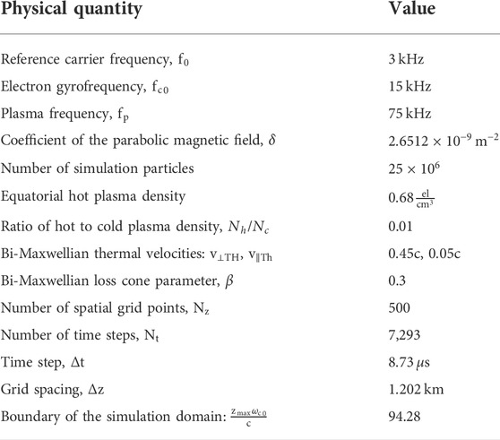
TABLE 1. Background, wave, and grid parameters used in the simulation.

Similar to the VHS formalism, the range of parallel velocities is limited such that they can resonate with waves between 2 and 4 kHz. The boundary condition for the particles follows “instantaneous mirroring” such that only the electron position is negated ($z\to -z$) if the parallel velocity exceeds the maximum limit or is below the minimum limit (corresponding to 4 and 2 kHz resonant waves, respectively), while all velocity components are conserved. The same condition is applied when electrons arrive at the left or right spatial boundaries of the simulation space. The wave boundary condition on the right hand side of the simulation enforces continuity of the derivative of the wave magnetic field (no injected wave), while the left hand side enforces simple outflow. The initial conditions on the wave magnitude are set identically to zero to ensure any generated waves are purely spontaneous. Furthermore, the envelope equations are updated with a backward semi-Lagrangian method, which, hence, circumvents the typical CFL stability condition. With all these simplifications, the E-PIC code runs approximately 5–10x faster than full PIC or hybrid PIC codes for this particular simulation setup.

The simulation generates a rising tone chorus element that is shown to be generated upstream of the equator. Figure 1 shows spectrograms of the wave fields at four locations along the field line that are upstream of the equator (opposite the direction of wave propagation). It is worth noting that the simulation results are shown in the same normalized space–time coordinates as employed by Hikishima et al. (2009). Specifically, Figure 1D shows a spectrogram of the wave furthest upstream ($\frac{z{\omega }_c}{c}=56.47$), and it is apparent that no frequency components are present. Figure 1C shows a spectrogram closer to the equator ($\frac{z{\omega }_c}{c}=37.58$), and it is apparent that a single frequency component is present at this point. Moving even closer to the equator ($\frac{z{\omega }_c}{c}=18.69$), additional lower frequency components are shown to appear at early points in time, and the rising tone structure is shown to emerge. Finally, at the equator (or numerically close at $\frac{z{\omega }_c}{c}=0.19$), the entire rising tone is present and represents a chorus element that will propagate and amplify downstream. Thus, as shown in Figure 1, the rising tone chorus element is mostly created upstream of the equator in the direction opposite to the wave’s propagation direction.

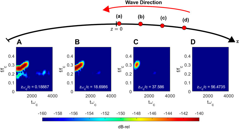
FIGURE 1. Spectrograms of the wave magnetic field starting at the (A) simulation equator and progressively more upstream (B,C,D).

The generation of the rising tone element occurs upstream of the equator; however, the initial “embryo” frequency emerges at the equator approximately at the maximum linear growth frequency (as suggested by Omura (2021)). Figure 2 shows four subplots where the y-axis corresponds to frequency, while the x-axis corresponds to position, and each subplot corresponds to a progressively increased point in time. Figure 2A shows the spatial distribution of frequency at $t{\omega }_C=81.85$.

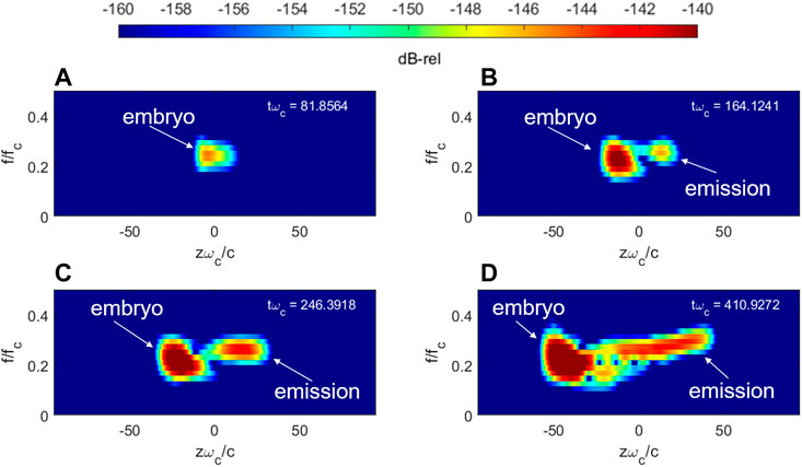
FIGURE 2. Spatial distribution of the wave frequency content during rising tone generation at progressively increasing snapshots in time. Earliest time (A) to latest time (D).

As shown, an initial embryo frequency emerges at the equator and propagates downstream at the frequency of maximum linear growth. It is also noticeable that the wavepacket “stretches” upstream to some extent, which serves as the initial point for the remainder of the rising tone. Figure 2B shows the frequency components a short time later at $t{\omega }_C=164.124$. It can be seen that a new higher frequency component emerges further upstream of the initial embryo. As time increases, as shown in Figures 2C,D, the remainder of the rising tone is generated while simultaneously propagating downstream, that is, the rising tone is sequentially generated upstream of the equator with the highest frequency components arising furthest downstream. It is worth noting that the emission eventually terminates at some point upstream (at approximately $\frac{z{\omega }_c}{c}=50$) and turns the emission into an “element”. However, it is currently unclear as to what underlying mechanism determines this termination point. It is potentially related to the “critical distance” described in Omura (2021); however, a detailed analysis of this is outside the current scope of this work.

It is worth noting that the embryo frequency component increases considerably in intensity (as shown by the dark red in Figures 2B–D) which is mostly a function of the artificially high anisotropy utilized in the simulation. This can be tuned in future works to determine the impact of the growth rate (and other parameters) on chorus generation.

Backward-propagating resonant current driving rising tone generation

The results shown in Figures 1, 2 clearly demonstrate that an embryonic component is generated at the equator, and the rising tone is subsequently generated upstream. However, it is still not immediately evident as to the mechanism by which the rising tone emerges. To assess a backward-moving source as a viable mechanism, a simple approach is via tracking the adiabatic trajectory of an initially de-trapped electron. Assuming that the embryo spontaneously emerges at the equator due to linear growth of thermal noise, the electrons that first encounter the embryonic wave from downstream will be phase-trapped and then rapidly ejected from the back end of the wavepacket. At this point, these de-trapped electrons now observe zero wave fields since they have been ejected into a region upstream where no waves exist. If the electrons have been phase-organized to any extent, as expected for phase-bunched electrons, for instance (where phase-bunching is based on the definition of Albert (2002)), a net current will be formed and a new wavepacket will be generated in its wake. Since the electrons are free falling out the back end of the wave, any “new” electrons that get trapped downstream by the freshly generated upstream wavepackets will already satisfy the local resonance condition and simply follow the trajectory of the electrons that were originally released by the embryo wave. At the same time, the waves are forced to be propagating in the forward (downstream direction) direction and will be supported by the resonant currents in the process. Thus, the constant flow of de-trapped electrons should result in a backward-going (i.e., upstream propagating) current that follows the adiabatic trajectory of the initially de-trapped electron stream superimposed with forward motion at the group velocity (as suggested by Nogi and Omura, (2022)). In order to confirm this hypothesis, the combined trajectory of adiabatic motion and group velocity motion can be calculated and compared to the hot current profile.

Assuming that the embryo wave generates at the frequency of maximum linear growth at the equator, the initially trapped electrons will have a parallel velocity equal to the local equatorial resonance velocity evaluated at the maximum linear growth rate frequency. From the equator, it can be assumed that electrons become quickly de-trapped and travel upstream adiabatically. The equation of motion governing the position of an electron, ${\mathrm{z}}_{\mathrm{a}}$, undergoing adiabatic motion after being released from resonance at the equator is given by

Here, the quantity ${\alpha }_{eq}$ is the pitch angle of the electron exactly at the equator. At the same time, the motion of the backward-propagating source must have the forward motion at the group velocity superimposed. Thus, the equation for the position of the backward-propagating source, $z_s$, is given by

Although the group velocity should also vary with time if the frequency of the wave changes, the E-PIC formalism currently does not include this effect (as mentioned in the previous section), and it is thus ignored in this post-processing calculation. For simplicity, we consider a fixed pitch angle within the range used in the simulation, that is, ${\alpha }_{eq}\approx 65°$. This value also falls within the pitch angle range expected to contribute to nonlinear growth (Nunn, 1990). The equation of motion shown in Eq. 12 can be numerically integrated to get the expected trajectory of the backward-moving source.

Figure 3 shows the space–time profile of the hot current magnitude (a), the wave magnetic field magnitude (b), and the wave’s instantaneous frequency (c), respectively. The instantaneous frequency is determined via the local maximum frequency on the spectrogram (using a 512-point FFT) and is only calculated for field amplitudes from 40 dB below the maximum amplitude up to the maximum amplitude (non-calculated points are shown in dark blue). As shown in Figure 3A, the hot current has a “V”-like structure that indicates both forward- and backward-going components. It should be noted that “backward” in this formalism corresponds to the component moving in the +z direction. On top of the space-time profile of the current, the source trajectory from integrating Eq. 12 is shown by the black curve. It is evident that the trajectory of an initially resonant electron with the group velocity subtracted out very closely aligns with the enhancement in the backward current. This strongly suggests that the backward stream of hot current is due to the repeated trapping and de-trapping process that, on average, follows the adiabatic trajectory of the initially de-trapped particle with the group velocity motion superimposed (with an opposite sign). The same trajectory is superimposed on the wave’s space–time profile in Figure 3B. It is evident that the expected trajectory of the source closely coincides with a backward-moving source that continuously radiates forward-going waves. Thus, the generation of the wave due to a backward-moving source that has also recently been shown by Nogi and Omura, (2022) in the context of VLF-triggered emissions that seem to also apply to the generation of whistler-mode chorus waves. It is also worth emphasizing that the source trajectory (Figure 3) is primarily utilized to visualize the average trajectory of the backward-going resonant current. The physically accurate picture is several successive bunches of particles that are constantly trapped and then de-trapped. This phenomenon is visible as the substructure in the resonant current profile in Figure 3A coincides with the source trajectory.

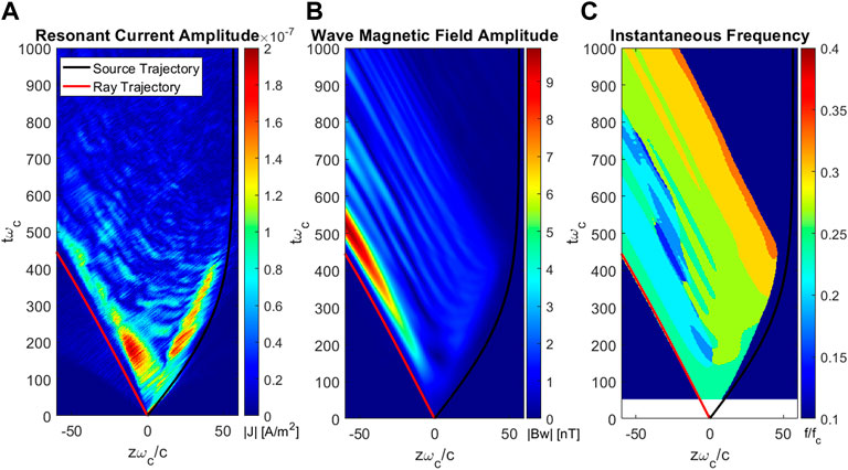
FIGURE 3. Space–time profiles of the (A) hot current density magnitude, (B) wave magnetic field magnitude, and (C) wave magnetic field instantaneous frequency. The source trajectory (Eq. 8) and the ray trajectory of a wave-front are superimposed as the black and red curves, respectively.

The envelope equation formalism of the E-PIC code only allows waves to propagate in the –z direction in the absence of any currents. Thus, the forward-going waves are expected to approximately follow the trajectory of a ray moving at the group velocity, which is superimposed as the red curve on all the panels of Figure 3. It is clear that the propagation of the wave does indeed follow the expected ray trajectory. The forward-going component of the current is more complex since it must transit from the backward component that radiates the wave to the forward component that sustains the wave after it has been generated. Finally, Figure 3C shows that higher frequency components are generated upstream of the equator and then propagate downstream to form the chorus element and undergo some nonlinear distortion. Furthermore, the initial generation of new frequency components is also shown to closely coincide with the theoretical source trajectory from Eq. 12.

The simulation results thus confirm that the rising tone whistler-mode chorus element is generated upstream of the equator due to a free falling electron stream that is de-trapped by a spontaneously generated equatorial embryonic wave.

Conclusion

Despite several decades of observational and theoretical investigation of magnetospheric chorus, there remains considerable debate on the precise mechanism of cyclotron resonance that governs the frequency chirp of chorus elements. A new E-PIC code has been developed to model chorus element generation in a parabolic magnetic field. We have shown that the chorus element initiates at the frequency of maximum linear growth at the equator. This embryo wave immediately phase-traps resonant electrons and releases them upstream. The de-trapped particles revert to adiabatic motion upstream of the equator, resulting in a backward-moving source. The motion of the backward-propagating source is consistent with the superposition of the adiabatic trajectory of an initially resonant electron and forward motion at the group velocity. Our results show that a blend of the conclusions by Tao et al. (2021) and Nogi and Omura (2022) seem to explain the origin of rising tone chorus elements. The results of this work thus provide valuable theoretical insight into the origin of the rising tone magnetospheric chorus.

Data availability statement

The original contributions presented in the study are publicly available. These data can be found at: Zenodo, https://doi.org/10.5281/zenodo.6565107, doi: 10.5281/zenodo.6565107.

Author contributions

All authors listed have made a substantial, direct, and intellectual contribution to the work and approved it for publication.

Conflict of interest

The authors declare that the research was conducted in the absence of any commercial or financial relationships that could be construed as a potential conflict of interest.

Publisher’s note

All claims expressed in this article are solely those of the authors and do not necessarily represent those of their affiliated organizations, or those of the publisher, the editors, and the reviewers. Any product that may be evaluated in this article, or claim that may be made by its manufacturer, is not guaranteed or endorsed by the publisher.

References

Albert, J. M. (2002). Nonlinear interaction of outer zone electrons with VLF waves. Geophys. Res. Lett. 29, 116-1–116-3. doi:10.1029/2001GL013941
Bell, T. F. (1984). The nonlinear gyroresonance interaction between energetic electrons and coherent VLF waves propagating at an arbitrary angle with respect to the Earth’s magnetic field. J. Geophys. Res. 89, 905–918. doi:10.1029/JA089iA02p00905
Birdsall, C. K., and Langdon, A. B. (2017). Plasma physics via computer simulation. Boca Raton: CRC Press. doi:10.1201/9781315275048
Bortnik, J., Thorne, R. M., and Meredith, N. P. (2008). The unexpected origin of plasmaspheric hiss from discrete chorus emissions. Nature 452, 62–66. doi:10.1038/nature06741
Crabtree, C., Ganguli, G., and Tejero, E. (2017). Analysis of self-consistent nonlinear wave-particle interactions of whistler waves in laboratory and space plasmas. Phys. Plasmas 24, 056501. doi:10.1063/1.4977539
Dysthe, K. B. (1971). Some studies of triggered whistler emissions. J. Geophys. Res. 76, 6915–6931. doi:10.1029/JA076i028p06915
Furuya, N., Omura, Y., and Summers, D. (2008). Relativistic turning acceleration of radiation belt electrons by whistler mode chorus. J. Geophys. Res. 113. doi:10.1029/2007JA012478
Gibby, A. R. (2008). Saturation effects in VLF triggered emissions (ph.D.). ProQuest dissertations and theses. United States -- California: Stanford University.
Gołkowski, M., and Gibby, A. R. (2017). On the conditions for nonlinear growth in magnetospheric chorus and triggered emissions. Phys. Plasmas 24, 092904. doi:10.1063/1.4986225
Gołkowski, M., Harid, V., and Hosseini, P. (2019). Review of controlled excitation of non-linear wave-particle interactions in the magnetosphere. Front. Astron. Space Sci. 6. doi:10.3389/fspas.2019.00002
Harid, V., Gołkowski, M., Bell, T., and Inan, U. S. (2014a). Theoretical and numerical analysis of radiation belt electron precipitation by coherent whistler mode waves. J. Geophys. Res. Space Phys. 119, 4370–4388. doi:10.1002/2014JA019809
Harid, V., Gołkowski, M., Bell, T., Li, J. D., and Inan, U. S. (2014b). Finite difference modeling of coherent wave amplification in the Earth’s radiation belts. Geophys. Res. Lett. 41, 8193–8200. doi:10.1002/2014GL061787
Helliwell, R. A. (1967). A theory of discrete VLF emissions from the magnetosphere. J. Geophys. Res. 72, 4773–4790. doi:10.1029/JZ072i019p04773
Hikishima, M., Yagitani, S., Omura, Y., and Nagano, I. (2009). Full particle simulation of whistler-mode rising chorus emissions in the magnetosphere. J. Geophys. Res. 114. doi:10.1029/2008JA013625
Hosseini, P., Gołkowski, M., and Harid, V. (2019). Remote sensing of radiation belt energetic electrons using lightning triggered upper band chorus. Geophys. Res. Lett. 46, 37–47. doi:10.1029/2018GL081391
Inan, U. S., Bell, T. F., and Helliwell, R. A. (1978). Nonlinear pitch angle scattering of energetic electrons by coherent VLF waves in the magnetosphere. J. Geophys. Res. 83, 3235–3253. doi:10.1029/JA083iA07p03235
Katoh, Y., and Omura, Y. (2011). Amplitude dependence of frequency sweep rates of whistler mode chorus emissions. J. Geophys. Res. 116. doi:10.1029/2011JA016496
Kennel, C. F., and Petschek, H. E. (1966). Limit on stably trapped particle fluxes. J. Geophys. Res. 71, 1–28. doi:10.1029/JZ071i001p00001
Lu, Q., Ke, Y., Wang, X., Liu, K., Gao, X., Chen, L., et al. (2019). Two-dimensional gcPIC simulation of rising-tone chorus waves in a dipole magnetic field. J. Geophys. Res. Space Phys. 124, 4157–4167. doi:10.1029/2019JA026586
Matsumoto, H. (1979). “Nonlinear whistler-mode interaction and triggered emissions in the magnetosphere: A review,” in Wave instabilities in space plasmas, astrophysics and space science library. Editors P. J. Palmadesso, and K. Papadopoulos (Dordrecht: Springer Netherlands), 163–190. doi:10.1007/978-94-009-9500-0_13
Meredith, N. P., Horne, R. B., Sicard-Piet, A., Boscher, D., Yearby, K. H., Li, W., et al. (2012). Global model of lower band and upper band chorus from multiple satellite observations: Global model of whistler mode chorus. J. Geophys. Res. 117, n/a. doi:10.1029/2012ja017978
Mozer, F. S., Agapitov, O. V., Blake, J. B., and Vasko, I. Y. (2018). Simultaneous observations of lower band chorus emissions at the equator and microburst precipitating electrons in the ionosphere. Geophys. Res. Lett. 45, 511–516. doi:10.1002/2017GL076120
Nogi, T., and Omura, Y. (2022). Nonlinear signatures of VLF-triggered emissions: A simulation study. JGR. Space Phys. 127, e2021JA029826. doi:10.1029/2021JA029826
Nunn, D. (1974). A self-consistent theory of triggered VLF emissions. Planet. Space Sci. 22, 349–378. doi:10.1016/0032-0633(74)90070-1
Nunn, D., and Omura, Y. (2012). A computational and theoretical analysis of falling frequency VLF emissions. J. Geophys. Res. 117. doi:10.1029/2012JA017557
Nunn, D., Omura, Y., Matsumoto, H., Nagano, I., and Yagitani, S. (1997). The numerical simulation of VLF chorus and discrete emissions observed on the Geotail satellite using a Vlasov code. J. Geophys. Res. 102, 27083–27097. doi:10.1029/97JA02518
Nunn, D., Santolik, O., Rycroft, M., and Trakhtengerts, V. (2009). On the numerical modelling of VLF chorus dynamical spectra. Ann. Geophys. 27, 2341–2359. doi:10.5194/angeo-27-2341-2009
Nunn, D. (2021). The numerical simulation of the generation of lower-band VLF chorus using a quasi-broadband Vlasov Hybrid Simulation code. Earth Planets Space 73, 222. doi:10.1186/s40623-021-01549-3
Nunn, D. (1990). The numerical simulation of VLF nonlinear wave-particle interactions in collision-free plasmas using the Vlasov hybrid simulation technique. Comput. Phys. Commun. 60, 1–25. doi:10.1016/0010-4655(90)90074-B
Omura, Y., Katoh, Y., and Summers, D. (2008). Theory and simulation of the generation of whistler-mode chorus. J. Geophys. Res. 113. doi:10.1029/2007JA012622
Omura, Y. (2021). Nonlinear wave growth theory of whistler-mode chorus and hiss emissions in the magnetosphere. Earth Planets Space 73, 95. doi:10.1186/s40623-021-01380-w
Omura, Y., Nunn, D., Matsumoto, H., and Rycroft, M. J. (1991). A review of observational, theoretical and numerical studies of VLF triggered emissions. J. Atmos. Terr. Phys. 53, 351–368. doi:10.1016/0021-9169(91)90031-2
Ripoll, J. ‐F., Claudepierre, S. G., Ukhorskiy, A. Y., Colpitts, C., Li, X., Fennell, J. F., et al. (2020). Particle dynamics in the earth’s radiation belts: Review of current research and open questions. J. Geophys. Res. Space Phys. 125. doi:10.1029/2019JA026735
Roux, A., and Pellat, R. (1978). A theory of triggered emissions. J. Geophys. Res. 83, 1433–1441. doi:10.1029/JA083iA04p01433
Summers, D., Omura, Y., Miyashita, Y., and Lee, D.-H. (2012). Nonlinear spatiotemporal evolution of whistler mode chorus waves in Earth’s inner magnetosphere. J. Geophys. Res. 117. doi:10.1029/2012JA017842
Summers, D. (2005). Quasi-linear diffusion coefficients for field-aligned electromagnetic waves with applications to the magnetosphere. J. Geophys. Res. 110. doi:10.1029/2005JA011159
Tao, X., Zonca, F., and Chen, L. (2021). A “trap-release-amplify” model of chorus waves. JGR. Space Phys. 126, e2021JA029585. doi:10.1029/2021JA029585
Tao, X., Zonca, F., and Chen, L. (2017). Identify the nonlinear wave-particle interaction regime in rising tone chorus generation. Geophys. Res. Lett. 44, 3441–3446. doi:10.1002/2017GL072624
Trakhtengerts, V. Y. (1999). A generation mechanism for chorus emission. Ann. Geophys. 17, 95–100. doi:10.1007/s00585-999-0095-4
Trakhtengerts, V. Y. (1995). Magnetosphere cyclotron maser: Backward wave oscillator generation regime. J. Geophys. Res. 100, 17205–17210. doi:10.1029/95JA00843
Vomvoridis, J. L., Crystal, T. L., and Denavit, J. (1982). Theory and computer simulations of magnetospheric very low frequency emissions. J. Geophys. Res. 87, 1473–1489. doi:10.1029/JA087iA03p01473
Wu, Y., Tao, X., Zonca, F., Chen, L., and Wang, S. (2020). Controlling the chirping of chorus waves via magnetic field inhomogeneity. Geophys. Res. Lett. 47, e2020GL087791. doi:10.1029/2020GL087791
Xiao, F., Liu, S., Tao, X., Su, Z., Zhou, Q., Yang, C., et al. (2017). Generation of extremely low frequency chorus in Van Allen radiation belts. J. Geophys. Res. Space Phys. 122, 3201–3211. doi:10.1002/2016JA023561
Keywords: magnetospheric chorus, particle–in-cell (PIC) simulation, wave generation, gyro-resonant interactions, electron de-trapping
Citation: Harid V, Gołkowski M, Hosseini P and Kim H (2022) Backward-propagating source as a component of rising tone whistler-mode chorus generation. Front. Astron. Space Sci. 9:981949. doi: 10.3389/fspas.2022.981949
Received: 29 June 2022; Accepted: 09 August 2022;
Published: 07 September 2022.
Edited by:
Yoshiharu Omura, Kyoto University, JapanReviewed by:
Xueyi Wang, Auburn University, United StatesShinji Saito, National Institute of Information and Communications Technology, Japan
Copyright © 2022 Harid, Gołkowski, Hosseini and Kim. This is an open-access article distributed under the terms of the Creative Commons Attribution License (CC BY). The use, distribution or reproduction in other forums is permitted, provided the original author(s) and the copyright owner(s) are credited and that the original publication in this journal is cited, in accordance with accepted academic practice. No use, distribution or reproduction is permitted which does not comply with these terms.
*Correspondence: Vijay Harid, vijay.harid@ucdenver.edu