Asteroid Photometric Phase Functions From Bayesian Lightcurve Inversion

1 Introduction

Asteroids are small Solar System objects that originate from times preceding planet formation. Typically, when rotating about its principal axis of inertia, an asteroid exhibits a periodic change of brightness caused by the varying part of its surface being both illuminated by the Sun and visible to the observer. On one hand, a photometric lightcurve is the result of photometric observations extending over a time span covering a substantial part of the rotation period or more. On the other hand, a photometric phase curve is the result of observations of the change in an asteroid’s apparent brightness obtained at different epochs during a single apparition, corresponding to a slowly changing Sun-observer-object geometry.

Consequently, photometric lightcurves provide immediate information about the rotation period. Historically, asteroid lightcurve observations have been the first tool intensively applied to derive physical properties of these objects. In addition to the retrieval of the rotation period, lightcurve amplitudes have been used to derive rough characteristics of the shape (elongated shapes generally producing lightcurves with larger amplitudes) and, when lightcurves obtained at different apparitions were available, to derive estimates of the direction of the asteroid’s pole orientation (Taylor, 1979; Magnusson et al., 1989; Kaasalainen et al., 2002; Durech et al., 2015). Some early statistical analyses of lightcurve amplitudes and periods led also to the discovery of the existence of equilibrium shapes among large asteroids (Farinella et al., 1981), and opened the way to the discovery of the importance of the general phenomenon of asteroid collisional evolution (Farinella et al., 1982).

Photometric phase curves provide information about the intrinsic light-scattering properties of the surface that are intimately related to the regolith composition and structure. Since the composition and structure determine also the reflectance properties observed at different wavelengths, phase curves are strictly related to the taxonomic classification of asteroids. Phase curves are often represented with the help of a few parameters. The classical two-parameter H, G magnitude system has been used for a long time (Bowell et al., 1989). H is the asteroid’s absolute magnitude, namely the magnitude (corresponding to unit distance from the Sun and the observer) measured at zero phase angle, and G is a parameter describing the overall variation of magnitude at different phase angles, including a nonlinear brightness surge at phase angles smaller than 10° (opposition effect). In recent years, it has been replaced by the so-called H, G₁, G₂ magnitude system, a three-parameter model developed by Muinonen et al. (2010) to remove the caveats of the H, G system in the case of low-albedo and high-albedo asteroids. Further refinements and applications of the H, G₁, G₂ system have been published, among others, by Penttilä et al. (2016) and Shevchenko et al. (2016).

Gaia Data Release 3 (DR3) is imminent (13 June 2022), including extensive astrometric, photometric, and spectroscopic observations of small Solar System objects, primarily asteroids. It is important to prepare to analyze such a large amount of new data. In the field of asteroid photometry, in particular, significant progress has been made recently in what concerns the capability of obtaining efficient processing and reliable interpretation of sparse photometric data. Martikainen et al. (2021) carried out an analysis of photometric data combined from ground-based lightcurves and observations published in Gaia Data Release 2 (DR2) in order to invert the data for reliable estimates of shape, rotational properties, and phase curves for a large number of objects belonging to a variety of asteroid taxonomic classes. They derived photometric phase curve slopes, rates of brightness change on the magnitude scale, for more than 300 asteroids in the so-called reference geometry of equatorial illumination and observation (Kaasalainen et al., 2001). Expanding on the study in Muinonen et al. (2020), Martikainen et al. (2021) provided unequivocal proof that the projection to similar illumination and observation conditions was needed to enable unbiased comparative studies of asteroid phase curves. It is possible to strive towards minimizing the biases by incorporating all practical geometries of illumination and observation (Oszkiewicz et al., 2011). However, for asteroids with their individual pole orientations and orbits, different illumination and observation geometries are sampled, and biases remain. In spite of these biases, Oszkiewicz et al. (2011) and Mahlke et al. (2021) have successfully related phase curve parameters from massive observing programs to the taxonomical classes.

We extend the work by Martikainen et al. (2021) by providing computational tools for the derivation of asteroid phase functions using fictitious spherical asteroids with equal surface properties. In earlier works, we have described these phase functions as being proper phase functions that describe the intrinsic properties of the surfaces. We apply the methods to the asteroids studied by Martikainen et al. (2021), by starting from their results of Markov-chain Monte Carlo (MCMC) lightcurve inversion for some 500 asteroids. Furthermore, we generalize the studies by Martikainen et al. (2021) and Muinonen et al. (2020) by incorporating a combined linear-exponential model of phase functions on the magnitude scale.

In earlier work (Muinonen et al., 2020), models of observational uncertainties were developed for dense relative photometry and sparse relative photometry. The former entailed ground-based lightcurves that were treated, in lightcurve inversion, on a relative magnitude scale. The latter comprised lightcurves of sparse Gaia photometry that were incorporated on a relative magnitude scale, too. Martikainen et al. (2021) then treated the Gaia photometry in the absolute sense, deriving absolute magnitudes for a large number of asteroids. In the present work, we provide a complete set of four models for observational uncertainties, including models for dense relative, sparse relative, dense absolute, and sparse absolute lightcurves.

The paper is organized as follows. Section 2 describes the theoretical framework in asteroid lightcurve inversion. Particular attention is paid to the different surface scattering models utilized in the forward and inverse problems. In Sect. 3, error models are presented for dense and sparse lightcurves (relative or absolute), and the retrieval of absolute magnitudes and phase functions is outlined. Section 4 first provides the application of the methods to ∼500 asteroids with both sparse absolute Gaia photometry and dense relative ground-based photometry. Thereafter, a numerical forward simulation of dense absolute photometry with a Gaussian-random-sphere asteroid model (GS-asteroid) is described, followed by inversion results and their discussion. Conclusions and future prospects are offered in Sect. 5.

2 Lightcurve Inversion

2.1 Asteroid Modeling

Consider an asteroid in principal-axis rotation. We denote the asteroid’s rotation period by P, the pole orientation in ecliptic longitude and latitude by (λ,β)^T (J2000.0, T stands for transpose), and the rotational phase at a given epoch t₀ by φ₀. As to the asteroid’s shape, in the inverse problem, we consider both ellipsoidal shapes and general convex shapes. In the forward problem, we incorporate star-like shapes described by the Gaussian-random-sphere geometry.

The apparent V-band magnitude (in mag) of a fictitious spherical asteroid (diameter D in km and geometric albedo pV) at a given phase angle α is

where H is the absolute magnitude (in mag), r and Δ are the asteroid’s heliocentric and topocentric distances (in au), Φ is the phase function (Φ(0°) = 1), and lg denotes the 10-based logarithm. The corresponding reduced V-band magnitude is projected to r = Δ = 1 au:

Scattering of light from a surface element on an asteroid is described by the diffuse reflection coefficient R that relates the incident solar flux density πF₀ to the emergent, scattered intensity I:

Here ι and ϵ are the angles of incidence and emergence as measured from the outward normal vector of the element, and ϕ₀ and ϕ denote the respective azimuthal angles. For a geometrically isotropic surface, it is unnecessary to specify ϕ₀ and we set the coordinate system so that ϕ₀ = 0°. Consequently, the backscattering direction, the direction for the source of light, is with ϕ = 0°.

The Lommel-Seeliger surface reflection coefficient (subscript LS) derives from radiative transfer (e.g., Lumme and Bowell, 1981):

where p is the geometric albedo for the wavelength band considered.

The diffuse reflection coefficient for dark particulate media (subscript PM)—such as planetary regoliths of low-albedo asteroids—can be expressed in the form (Muinonen et al., 2011; Wilkman et al., 2015)

where p is the geometric albedo, α is the phase angle, and $\tilde{\omega }$ and P₁₁ are the single-scattering albedo and single-scattering phase function (different from the phase function of the asteroid). The function Φ_S represents the corrections to radiative transfer due to the dense packing of the particulate medium, for example, the corrections due to shadowing among the particles typically much larger than wavelength. Φ₁₁ and Φ_S, as all functions Φ of the present study, are normalized to unity at backscattering:

The reflection coefficient in Eq. 5 belongs to a class of photometric models consisting of a Lommel-Seeliger-type volume-element part and a part describing scattering among volume elements in a particulate medium (e.g., Lumme and Bowell, 1981; Muinonen and Lumme, 1991).

Wilkman et al. (2015) provide an extensive set of numerical computations of the dense-packing correction Φ_S using particulate media of opaque spherical particles. They complete the modeling with the help of a fractional-Brownian-motion model for the roughness of interface between the medium and free space. There are altogether three parameters: the packing density of the particles v, the fractal Hurst exponent H_fBm, and the amplitude σ_fBm. Smaller H_fBm and higher σ_fBm imply rougher interfaces with stronger effects of interface roughness. The function Φ_S is an unknown function for asteroid surfaces. In what follows, as in Muinonen et al. (2015), we utilize Φ_S estimated for the lunar mare regolith by Wilkman et al. (2014).

Consider next the function Φ₁₁ in Eqs 4, 5 and the large numbers of existing phase curve observations of asteroids. Indeed, we may consider that the principal form for the phase function of a fictitious spherical asteroid is already known to be described by, for example, the H, G₁, G₂ phase function. Consequently, we introduce denominators in Eqs 4, 5 that cancel the inherent phase function that would result from the assumption of Φ₁₁ = 1 (isotropic scattering):

where Φ represents an unknown function that should nevertheless be close to the empirically known phase functions of asteroids. In other words, the functions Φ_LS and Φ_PM are the phase functions for a spherical asteroid with reflection coefficients R_LS and R_PM assuming Φ₁₁ = 1, respectively. Figure 1 depicts the lunar disk-integrated phase function with the help of the H, G₁, G₂ phase function as well as the phase function Φ_PM derived for the lunar mare regions by Wilkman et al. (2015). Their ratio is also given. By approximating that Φ_PM can be valid for the higher-albedo lunar highland regions, too, the ratio points to the part of the lunar opposition effect at small phase angles unexplained by shadowing and rather explained by the coherent backscattering mechanism (Muinonen et al., 2002). Significantly different single-scattering phase functions Φ/Φ_LS or Φ/Φ_PM result from utilizing R_LS or R_PM: as R_PM assigns a significant part of phase curve steepness to shadowing, the resulting single-scattering phase function is shallower.

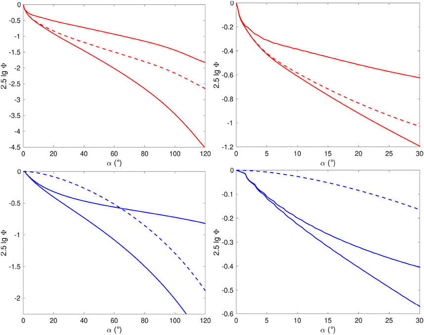
FIGURE 1. Phase functions and their ratios on the magnitude scale. The red curves (top left and right) correspond to the lunar phase function Φ (lowermost solid line), the ratio Φ/Φ_LS (middle dashed line), and the ratio Φ/Φ_PM (uppermost solid line; see Eq. 7). The blue curves (bottom left and right) denote Φ_PM (lowermost solid line), Φ_LS (at α = 120°, middle dashed line), and Φ_PM/Φ_LS (at α = 120°, uppermost solid line). The raggedness at small phase angles is an artefact deriving from the interpolation of Φ_PM.

In order to model the function Φ in Eq. 7 for lightcurve inversion, we make use of a linear-exponential model on the magnitude scale:

where m₀ and α₀ are the amplitude and angular width of the opposition effect, respectively, and β₀ is a slope parameter. In the linear-exponential model of Eq. 8, the photometric slope at α = 20° (the phase angle chosen for comparative studies) equals

For phase angles outside the angular regime of the opposition effect, 10° ≤ α ≤ 50°, a linear model can be utilized:

The H, G₁₂ phase function is a two-parameter phase function developed for scarce photometric data (Muinonen et al., 2010). As in Martikainen et al. (2021), we rule out increasing brightness with increasing phase angle and enforce the absence of an opposition effect for G₁₂ values that would result in negative weights 1 − G₁ − G₂:

The extension does not affect the H, G₁₂ phase function within its approximate nominal range of 0 ≤ G₁₂ ≤ 1.

2.2 Inverse Problem

Consider the free parameters (unknowns) of the asteroid forward model. In the case of the ellipsoid shape model, the parameters are described by the vector

where the N_P = 9 free parameters are, respectively, the rotation period, ecliptic pole longitude, ecliptic pole latitude, rotational phase at a given epoch t₀, two ellipsoid axial ratios (with a > b > c denoting the semiaxes), and three parameters of the linear-exponential phase function. In the case of the convex shape models, the parameters are

where the shape is described by the ${(l_{\text{max}}+1)}^2-l_{\text{min}}^2$ spherical harmonics coefficients $s_{00},\dots ,s_{l_{\text{max}}{l}_{\text{max}}}$ for the Gaussian surface density. Here φ₀ and the real-valued s₀₀ can be fixed as the rotational phase is immersed in the spherical harmonics coefficients and the asteroid size information is omitted. Thus, the total number of parameters equals

Let p_p be the a posteriori probability density function (p.d.f.) for the parameters. Within the Bayesian framework (cf. Muinonen et al., 2020), p_p is proportional to the a priori and observational uncertainty p.d.f.s p_pr and p_ϵ+υ, ϵ and υ referring to random and systematic uncertainties. p_ϵ+υ is evaluated for the “Observed-Computed” (O-C) residual magnitudes ΔM(P),

Even though p_ϵ+υ is here related to the observations, it can also describe the uncertainties deriving from the shortcomings in the physical model. It is currently assumed that p_ϵ+υ is Gaussian and that p_pr will describe, for example, the regularization needed in convex inversion. The final a posteriori p.d.f. is thus

where χ² measures the O-C distance in terms of the model for the uncertainties. The observation vector is composed of a number of lightcurves with their varying numbers of magnitudes, and the uncertainties are assumed to be uncorrelated between the lightcurves. We may thus rephrase χ²(P) as

where M_obs,k, M_k(P), and Λ_ϵ+υ,k pertain to the observations, computations, and the covariance matrix for the uncertainties in lightcurve k, the total number of lightcurves being K.

In detail, we simplify the χ²-value in Eq. 17 to the form

where the σ_ϵ,k values describe the uncertainty (and weight) of the N_k observations in lightcurve k, and M_obs,kj and M_kj(P) are the observed and computed magnitudes. For small relative uncertainties in brightness, the χ²-value can be approximated by (Muinonen et al., 2020)

where ΔM_k0(P) denote the O-C difference of the mean magnitudes in lightcurve k, and ℓ_obs,kj and ℓ_kj(P) are the observed and computed brightnesses relative to the brightnesses corresponding to the lightcurve mean magnitude lg∼e 0.43429. Thus, in Eq. 19, the χ²-value is computed using the differences in the observed and computed relative brightnesses, relative to the observed relative brightnesses.

3 Numerical Methods

The MCMC inverse methods are based on proposal probability densities characterized with the help of the so-called virtual least-squares solutions and are described in detail by Muinonen et al. (2020). In what follows, we introduce the error models for the observations and the algorithm for the retrieval of absolute magnitudes and phase functions from DR2 photometry.

3.1 Error Models for Observations

We define dense lightcurves as having photometric points timed, on average, less than the asteroid’s estimated rotation period apart. For dense relative lightcurves, the points are calibrated against each other but not against absolute standards. We set (Muinonen et al., 2020)

where σ_0,k denotes the rms-value and σ_pr,k denotes the a priori threshold value for the uncertainty in the lightcurve k, obtainable, for example, from cubic spline fits to the lightcurves. Furthermore, ΔT_k is the mean sampling time interval of the lightcurve k,

where $\tilde{k}$ marks the lightcurve with the lowest sampling rate in time and T_k stands for the time span of the lightcurve k. Equation 20 can be interpreted in the following way. The lightcurve $\tilde{k}$ contributes a χ²-value of unity in the inverse problem, whereas each other lightcurve k is considered to split into approximately N_k,eff independent lightcurves.

For dense absolute lightcurves composed of K lightcurves, the points are calibrated both against each other and absolute standards. We start by setting

where σ_0,k and σ_pr,k are defined as for Eq. 20. The definition of N_k,eff is the key point of the error model. For simplicity, consider the case σ_0,k ≥ σ_pr,k. First, if we set N_k,eff = 1, each lightcurve obtains an equal weight of unity. This is the most conservative model with systematic errors dominating over the random errors. Second, we may set N_k,eff = 1 for the lightcurve $\tilde{k}$ that has the minimum number of observations and consider the other lightcurves as composed of an effective number of

lightcurves like lightcurve $\tilde{k}$, balancing the weights of lightcurves with drastically different numbers of observations. We recall that the systematic errors include, in addition to the observational errors, the effects of simplified forward modeling, in particular, for the phase function in Eqs 8–10.

We define sparse lightcurves as having photometric points timed, on average, more than the estimated rotation period apart. For sparse relative lightcurves, as for dense relative lightcurves, the points are calibrated against each other but not against absolute standards. In accordance with Muinonen et al. (2020), we set $N_{k,\mathrm{e}\mathrm{ff}}=N_{\tilde{k}}$ in an error model coinciding with the form in Eq. 22, the index $\tilde{k}$ now denoting the sparse lightcurve with the smallest number of observations. Finally, for sparse absolute lightcurves, we introduce a model that coincides with the one for the sparse relative lightcurves. Now the observations are, however, calibrated against absolute standards.

The complete a posteriori p.d.f. is the product of the p.d.f.s for the four classes so that the corresponding χ²-values are added together:

or

where the index i describes the dense relative (i = 1), sparse relative (i = 2), dense absolute (i = 3), and sparse absolute photometry (i = 4). For dense and sparse relative lightcurves, the relative brightnesses ℓ_obs,ikj and ℓ_ikj(P) are computed using the mean-magnitude brightnesses of each lightcurve. However, for dense and sparse absolute lightcurves, they are computed using the mean magnitude of the entire absolute lightcurve data. Note that the sparse relative lightcurves are weighted equally to the absolute photometric data but they enter the inverse problem separately with no regard to the absolute level of brightness.

3.2 Absolute Magnitudes and Phase Functions

We refine the algorithm in Martikainen et al. (2021) for the derivation of absolute magnitudes and phase functions from Gaia photometry. As in their study, first, we start from the phase function slope parameter β_S retrieved from MCMC inversion, recalling that β_S describes the intrinsic surface-element properties of an asteroid. Second, using the full asteroid model available from the inversion, we move to the reference geometry of equatorial illumination and observation at the epochs and phase angles of the individual photometric points. Third, by computing the asteroid model brightnesses over one full rotation for each epoch, we determine the magnitudes of lightcurve brightness maxima. Martikainen et al. (2021) then carried out linear least-squares fitting to determine their phase curve slope parameter β_max, from which they derived the full H, G₁₂ phase function. As a small improvement, we fit, directly, the H, G₁₂ phase function to the magnitudes of the brightness maxima. The resulting H and G₁₂ parameters then allow us to predict the lightcurve brightness maxima at arbitrary phase angles within 0°–120°. Fourth, a reference phase curve is computed for selected phase angles by averaging the magnitudes over one full rotation. Fifth, magnitudes of lightcurve brightness maxima are computed for the selected phase angles, together with the values for the integrated disk function (∝ μ₀/(μ + μ₀) in Eqs 3, 4) and single-scattering phase function, all in the magnitude scale for the geometries corresponding to the brightness maxima. Sixth, a phase function is computed for an equal-projected-area spherical asteroid with the help of the single-scattering phase function, made possible by the fact that the mean projected area of a convex object in random orientation is one fourth of its total surface area (van de Hulst, 1957). An absolute magnitude then follows from the prediction to zero phase angle. Seventh, we fit the equal-sphere phase function using the full H, G₁, G₂ phase function. Finally, we compute the slopes of the mean-magnitude reference phase curve (β_ref) and the phase function (β_S) at the 20° phase angle. Repeating the computations above for all the MCMC solutions allows us to obtain uncertainty estimates for the absolute magnitudes and phase functions throughout the entire phase curve analysis.

4 Results and Discussion

The inverse methods are here applied to the ∼500 asteroids with ground-based and Gaia DR2 lightcurve data and to the simulated lightcurve data of the GS-asteroid.

4.1 Asteroids of Gaia Data Release 2

Martikainen et al. (2021) carried out MCMC convex lightcurve inversion for some 500 asteroids with photometric data deriving from Gaia DR2. In the present study, we make use their 5,000 MCMC samples for each asteroid and revisit the photometric phase function retrieval with improvements described in Sections 2 and 3. The number of successful phase function retrievals increased and 13 new asteroids were incorporated into the analysis, bringing the total number of successful retrievals to 358. The improvements further allowed us to derive uncertainties for the reference phase curves and final equal-sphere phase functions and absolute magnitudes. Whereas Martikainen et al. (2021) documented photometric slopes at 20° phase angle for the reference geometry of equatorial illumination and observation, we proceed to provide the full photometric phase function of a fictitious spherical object with surface scattering properties equal to those of the asteroid. Note that the earlier work addressed the estimation of the equal-sphere photometric slope across the phase-angle range of the Gaia observations, by incorporating the corresponding slope parameter in MCMC lightcurve inversion. As the phase-angle ranges differed for each asteroid, the slopes also differed a priori, sometimes substantially. The remedy utilized by Martikainen et al. (2021) was to move to the reference geometry and project the photometric slopes to the same phase angle of 20°. Due to the fact that, in the reference geometry, we replace the linear model by the H, G₁₂ phase function and repeat the analysis separately for each MCMC sample solution, we are capable of carrying out the analysis of uncertainties all the way to the equal-sphere phase functions. Complete tables including all the present results for the Gaia DR2 phase functions are available from the authors.

Figure 2 shows example lightcurves for asteroid (167) Urda together with best-fit convex model predictions and MCMC uncertainty envelopes. The sparse Gaia DR2 lightcurve is accurately modeled with realistic model uncertainties. Modeling for the dense ground-based lightcurve is satisfactory. Figure 3 presents histograms of the β_S (20°) and β_ref values that were obtained for 358 asteroids. To reiterate, β_S(20°) refers to the photometric slope from equal-sphere phase function obtained at the 20° phase angle, and β_ref refers to the slope of the mean-magnitude reference phase curve at the same phase angle. The β_ref values show no significant differences compared to the values derived in the previous study by Martikainen et al. (2021). The values of β_S and β_ref range from 1.3 to 5.3 mag/rad and are almost identical which can be seen in Figures 3, 4 with the exception of two noticeable outliers. The asteroid (15172) 3086 P-L shows a deviation of 0.19 mag/rad. It has only 3 lightcurves with a total of 398 observations. The phase-angle range of the Gaia lightcurve is 8°. Asteroid (5902) Talima shows a slightly larger deviation of 0.23 mag/rad. It has only 3 lightcurves totaling 29 observations. Again, the phase-angle range of the Gaia lightcurve is 8°. For these objects, the small number of ground-based lightcurves gives rise to large uncertainties.

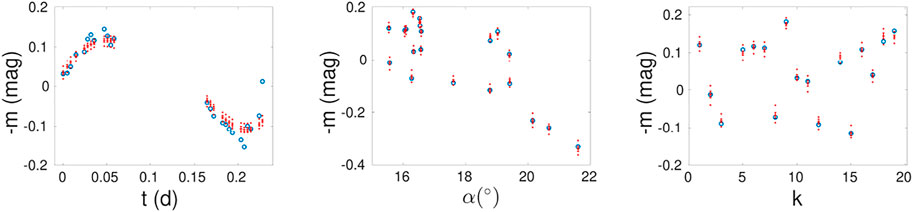
FIGURE 2. Example photometric lightcurves for asteroid (167) Urda (blue circles) on the magnitude scale. We show the ground-based dense lightcurve #8 (left) and the Gaia sparse lightcurve (middle and right). Red crosses stand for the best-fit convex model lightcurves with the 1-σ uncertainties (red bars), and the red points are the uncertainty envelopes using 5,000 MCMC sample solutions. The symbols t, α, and k denote the time, phase angle, and lightcurve observation counter.

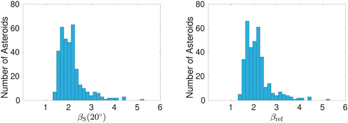
FIGURE 3. Histograms of the derived β_S(20°) and β_ref values (both in mag/rad), obtained using 358 asteroids.

FIGURE 4. Comparison of the derived β_S(20°) and β_ref values using 358 asteroids. The blue line represents perfect correlation. Two noticeable outliers (5902) Talima and (15172) 3086 P-L are marked with blue crosses.

For the vast majority of the asteroids presently studied, the absolute magnitude referring to random orientation is brighter than the absolute magnitude referring to the reference geometry. The explanation derives from a bias in the reference geometry. For the sake of clarity, let us characterize the shape of the asteroid by the semiaxes a ≥ b ≥ c as in the ellipsoidal model. On one hand, in the reference geometry, an asteroid rotating about its axis c of maximum inertia will never be viewed with its maximum projected area pointing in equatorial directions, whereas, in random orientation, maximum-projected-area viewing is enabled. Consequently, the asteroid exhibits a larger mean projected area in random orientation than in the reference geometry and the resulting absolute magnitude is brighter. On the other hand, in the reference geometry, in the unlikely case of an asteroid rotating about its long axis a of minimum inertia, there is a bias towards the asteroid appearing larger in the reference geometry than in random orientation. As most of the asteroids are rotating about their axis of maximum inertia, at the population level, the absolute magnitude is predominantly brighter in the case of random orientation.

In Figure 4, we compare the β_S (20°) and β_ref values. For every asteroid, the value of the β_ref is marginally greater than or equal to the value of β_S (20°). The explanation can again be related to a bias in the reference geometry. There, the minimum projected area of an ellipsoidal asteroid appears in equatorial viewing. Recalling the increase of lightcurve amplitude with phase angle assessed by Zappalà et al. (1990), the reference geometry provides the steepest phase curve dependence available for lightcurve brightness minima of a given asteroid. As to the lightcurve brightness maxima, phase curve dependences shallower than those in the reference geometry are available in random orientation, as geometries involving the maximum projected area of the asteroid are exposed. It is reasonable that the mean-magnitude reference phase curve turns out to be steeper than the mean-magnitude random-orientation phase curve. Conversely, for asteroids rotating about their axis of minimum inertia, the random-orientation phase curves are steeper than the reference phase curves.

The uncertainties for β_S (20°) as a function of β_S (20°) itself are depicted in Figure 5. Martikainen et al. (2021) showed that, despite of all the asteroid classes overlapping with each other to an extent, the C-complex and the S-complex asteroids form their own distinctive groups. This can be seen more clearly in our results: the C-complex asteroids have larger β_S(20°) values and are located on the right, whereas the S-complex asteroids have smaller β_S(20°) and are located on the left. The X-complex and end member asteroids are spread more widely as both groups are heterogeneous, containing asteroids with different albedos and compositions. In the middle and bottom panel of Figure 5, we focus for simplicity on the Tholen taxonomic classification, and do not check the possibility that some of the objects could belong to a different class according to more modern taxonomic classifications.

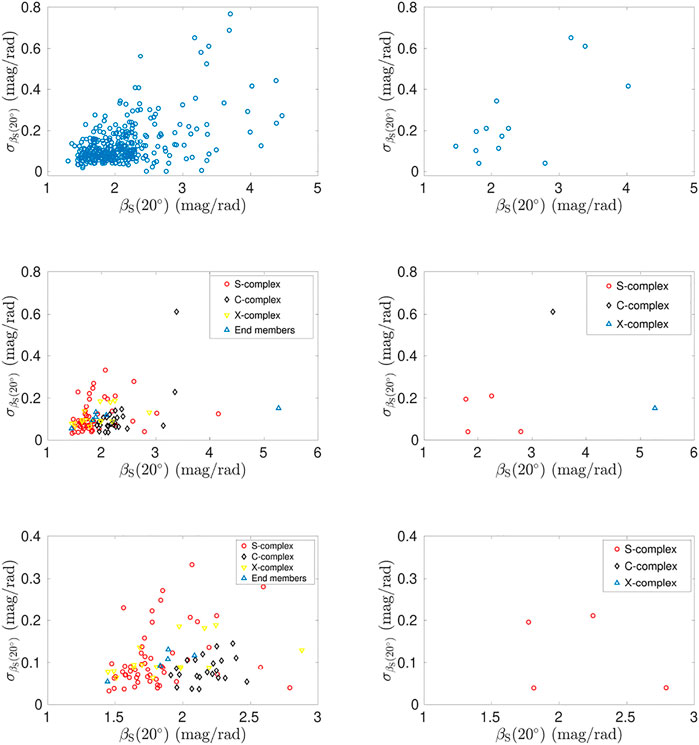
FIGURE 5. The topmost graphs depict ${\sigma }_{{\beta }_{\text{S}}(20°)}$ as a function of β_S(20°) using 358 asteroids (left) and highlighting 13 new asteroids presently processed (right). The middle graphs show ${\sigma }_{{\beta }_{\text{S}}(20°)}$ as a function of β_S(20°) for 97 asteroids with known Tholen classes (left), highlighting six new asteroids (right). The bottom graphs provide a zoom-in of the middle graphs.

The relation between the derived G-band absolute magnitudes G(1,0) and the V-band absolute magnitudes H for the 358 asteroids is displayed in Figure 6. The V-band absolute magnitudes were retrieved from the Jet Propulsion Laboratory Small-Body Database. The figure shows that our derived G-band magnitudes are nearly perfectly correlated save for a few outliers. These are most likely caused by insufficient lightcurve data. Asteroid (1368) Numidia shows a deviation of 0.81 mag from its respective H value, and has only 4 lightcurves that totaled in 40 observations. The phase-angle range of the Gaia lightcurve is only 4°, which is bound to result in uncertainties. Asteroid (446) Aeternitas shows the largest deviation of 1.37 mag. Despite having 128 lightcurves totaling 1794 observations, the phase-angle range of the Gaia lightcurve is again just 4°.

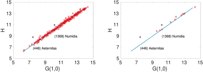
FIGURE 6. Comparison of the derived equal-sphere G-band absolute magnitudes G(1,0) and the V-band absolute magnitudes H based on the Jet Propulsion Laboratory Small-Body Database for 358 asteroids (left), the right panel highlighting the 13 new asteroids. The blue line represents perfect correlation of the absolute magnitudes. Two noticeable outliers (446) Aeternitas and (1368) Numidia are marked with blue crosses.

Table 1 describes the taxonomical classes, numbers of observations, and phase-angle ranges for 12 example asteroids chosen for a more detailed study as in Martikainen et al. (2021). Thereafter, Figure 7 showcases the random-orientation phase functions along with the H, G₁, G₂ fits for asteroids (55) Pandora, (95) Arethusa, (245) Vera, (596) Scheila, (731) Sorga, and (1251) Hedera. These asteroids were chosen to demonstrate different Tholen classes and to compare our results to the phase functions shown in Martikainen et al. (2021). The H, G₁, G₂ phase functions were fitted using the phase angles of 0.0°, 0.3°, 1.0°, 4.0°, 8.0°, 12.0°, 20.0°, 30.0°, and 50.0°. A noticeable change to results by Martikainen et al. (2021) comes up in the order of the phase functions in terms of their slope at 20°. In particular, the asteroids (245) Vera and (1251) Hedera have exchanged places. We are still involved in analyzing scarce Gaia DR2 data and expect to be able to offer more solid conclusions based on the forthcoming Gaia DR3 data.

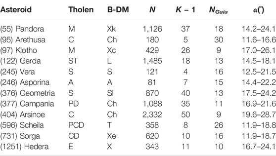
TABLE 1. Example asteroids with photometry in Gaia Data Release 2. Tholen stands for the Tholen taxonomic class, B-DM stands for the Bus-DeMeo taxonomic class, N is the total number of Gaia and ground-based observations, K − 1 is the number of observed ground-based lightcurves, N_Gaia is the number of observed Gaia points, and α denotes the phase angle coverage for each asteroid using Gaia data.

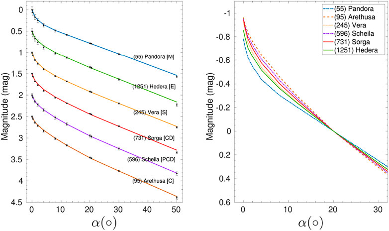
FIGURE 7. Photometric phase functions with H, G₁, G₂ -fits for asteroids (55) Pandora (95) Arethusa (245) Vera (596) Scheila (731) Sorga, and (1251) Hedera. For illustration, the phase functions are presented on a relative magnitude scale with 0.5-mag offsets (left) and normalized at 20° (right).

Table 2 provides a detailed comparison, including uncertainties, of the phase function slopes β_S, β_ref, and β_S (20°). It is clear that the latter two are closer to one another than to β_S that has been computed over a different phase-angle range for each asteroid. When comparing to phase-angle ranges documented in Table 1, a systematic behavior is seen: for phase-angle ranges located towards phase angles smaller than 20°, those local slopes are higher than the slope β_S(20°). This derives from the smoothly onsetting opposition effect prominent at small phase angles. For phase-angle ranges centered near 20°, the two slopes are similar. Finally, asteroid (245) Vera shows a phase function strikingly similar to that of the Moon. In Table 3, absolute magnitudes with uncertainties are collected for all 12 example asteroids. For most of the asteroids, the reference absolute magnitude is fainter than the random-orientation one, but there are two exceptions, (246) Asporina and (1251) Hedera. Whether these asteroid rotate about their axes of minimum inertia remains as an open question that may well be resolved by the forthcoming Gaia DR3 data.

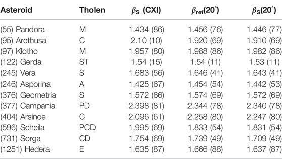
TABLE 2. The photometric slope β_S (mag/rad) of the phase function retrieved using convex inversion by Martikainen et al. (2021) (CXI), together with the mean-magnitude reference phase curve slope β_ref (mag/rad) and the slope β_S (mag/rad), both computed for the phase angle of 20°. All the slope parameters represent the means from MCMC sampling. The uncertainties are given in units of the last digit shown.

TABLE 3. The Tholen classes, the derived G-band absolute magnitudes G_RG(1,0) and G_EQ(1,0) for the reference geometry and equal-sphere case, respectively, the derived absolute magnitudes H_G using the H, G₁, G₂ fit, and the derived G₁ and G₂ parameters for the equal-sphere photometric phase functions. The uncertainties are given in units of the last digit shown.

We present the derived G₁ and G₂ parameters for the different Tholen classes in Figure 8 together with the G₁₂ parameter mapping to G₁ and G₂ in the H, G₁₂ magnitude system. It is possible to distinguish three groups in the G₁, G₂ parameter space: the first group contains the M and S classes, the second group contains the D class, and the third group consists of the C, G, and F classes. The figure also includes A, P, X, and B classes that each contains a single asteroid. Our results differ from those of Martikainen et al. (2021) as they pointed out only two distinctive groups. The updated computations suggest that, for the M and S classes, the G₁ parameter is smaller and the G₂ parameter is larger, moving the group toward the upper left. The opposite happens to the third group as the G₁ parameter is larger and the G₂ parameter smaller than in the previous computations moving the group to the lower right. As above, we must emphasize the preliminary nature of the studies by us and Martikainen et al. (2021), due to the scarce data available. We also recall that, in producing the plot in Figure 8, we did not check the possibility that, according to more modern taxonomic classifications, some of the objects we have analyzed could belong to a different class.

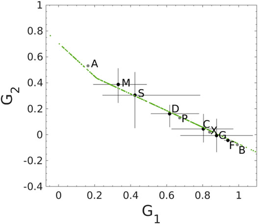
FIGURE 8. The distributions of the different Tholen classes (black dots) and their range (black crosses) in the G₁ and G₂ parameter space based on the equal-sphere phase functions. The grey dots represent single asteroids and the green line shows how the G₁₂ parameter maps into G₁ and G₂ in the H, G₁₂ magnitude system.

4.2 Gaussian-Sphere Asteroid

The Gaussian-random-sphere asteroid simulation is carried out using the observational cadence of asteroid (26) Proserpina both for the Gaia DR2 and ground-based observations (Durech et al., 2010; Gaia Collaboration et al., 2018; Muinonen et al., 2020). It involves the shape and rotation model in Torppa and Muinonen (2005) and the so-called lunar mare surface scattering model (Muinonen et al., 2015; Wilkman et al., 2015) of the form in Eq. 5. The asteroid is assumed to have a photometric phase function coinciding with the H, G₁, G₂ fit to the lunar phase curve (Muinonen et al., 2010). Basic information about the simulated observations is offered in Table 4. Zero-mean Gaussian random errors with a standard deviation of 0.01 mag were added to the numerically integrated magnitudes.

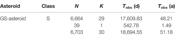
TABLE 4. Lightcurve characteristics for the simulated Gaussian-sphere asteroid (GS-asteroid). “Class” denotes the Tholen taxonomical class, N and K denote the numbers of observations and lightcurves, respectively, and T_obs is the time span of the observations. The uppermost numbers refer to the simulated dense ground-based observations, the ones in the middle to the simulated sparse observations, and the lowermost ones refer to the combined observations.

There are 29 dense lightcurves with altogether 6,664 data points and a single sparse lightcurve with 39 data points simulated for the GS-asteroid (Table 4). The total number of points is thus 6,703, spanning more than 51 years. The data set covers a phase-angle range from 1.77° to 21.62°, altogether 19.85°. Note that the single sparse lightcurve covers the phase angle range of ∼14–22° and does not constrain the opposition effect. Table 5 describes the properties of the individual lightcurves in terms of their time spans, mean sampling time intervals, and number of data points. Additionally, cubic spline fits dictated by the Bayesian Information Criterion (Liddle, 2007) for the numbers of evenly spaced spline nodes are presented for each lightcurve. The rms-values of the fits are in agreement with the 0.01-mag standard deviation used to simulate the errors.

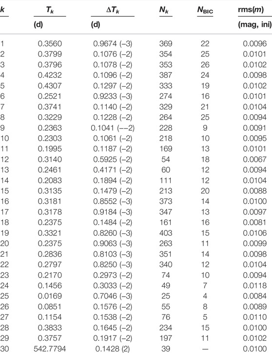
TABLE 5. Lightcurve characteristics for the simulated GS-asteroid. First, we give the lightcurve identifier (k), time span (T_k), mean sampling time interval (ΔT_k), and number of observations (N_k). Second, we give the number of nodes for the cubic spline fit based on the Bayesian information criterion (N_BIC) and the rms-value of the spline fit in relative magnitude (rms(m)). In the third column, for example, 0.9674 (−3) stands for 0.9674 × 10^–3.

Lightcurve inversion for the GS-asteroid data was carried out using Lommel-Seeliger ellipsoids and general convex shapes for two principal cases: one where all of the lightcurves were assumed to represent relative photometry and the other where all were assumed to represent absolute photometry. In addition, two error models were studied for each of the principal cases: the first model assigned a unit weight for each ground-based lightcurve, whereas the second model differed for the relative and absolute photometry as described in Section 3. Consequently, the analysis consisted of 8 different case studies.

In the case of convex inversion, after in-depth studies using least squares and MCMC, the error model for relative photometry was chosen to be the conventional one presented in Muinonen et al. (2020), whereas the error model for absolute photometry was taken to be the one with a unit weight for each dense ground-based lightcurve. The latter, conservative error model was required to account for, primarily, the systematic errors arising from the forward modeling of the inverse problem. Likewise, in ellipsoid inversion concerning both relative and absolute photometry, a unit weight was assigned for each dense ground-based lightcurve.

Least-squares fitting and MCMC sampling were carried out for all cases. In final MCMC inversion, 30,000 samples were computed using Lommel-Seeliger ellipsoids and 30,000 samples were computed using general convex shapes. Altogether, of the order of a month of sequential CPU time was required. Tables 6, 7 describe, for convex inversion, the details of the initial and final models of uncertainties in the cases of relative photometry and absolute photometry, respectively. The tables include the effective number of observations for each lightcurve, to be compared to the actual number of observations (Table 5). The final rms-values on the magnitude scale indicate that, even with convex inversion, the goodness of fit cannot reach the standard deviation used to simulate the errors. This is due to the forward modeling incorporated in the inversion, in particular, due to the restrictive linear-exponential phase function and the pure Lommel-Seeliger scattering model. Indeed, we can see that the fits are better for the case of relative photometry, due to the less stringent requirements on the phase function.

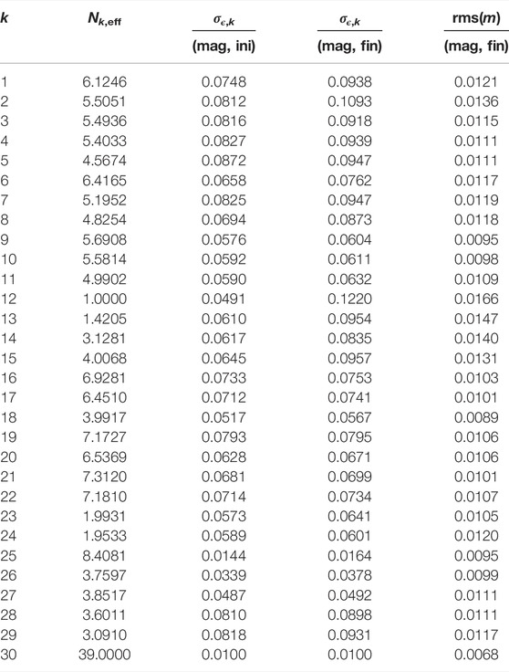
TABLE 6. Lightcurve characteristics for the GS-asteroid in the case of relative photometry. First, we give the lightcurve identifier (k), effective number of observations (N_k,eff, Eq. 20), and the resulting initial uncertainties (σ_ϵ,k, “ini”). Second, we give the final uncertainties (σ_ϵ,k, “fin”) and rms-values (rms(m), “fin”) for the best-fit model from convex inversion.

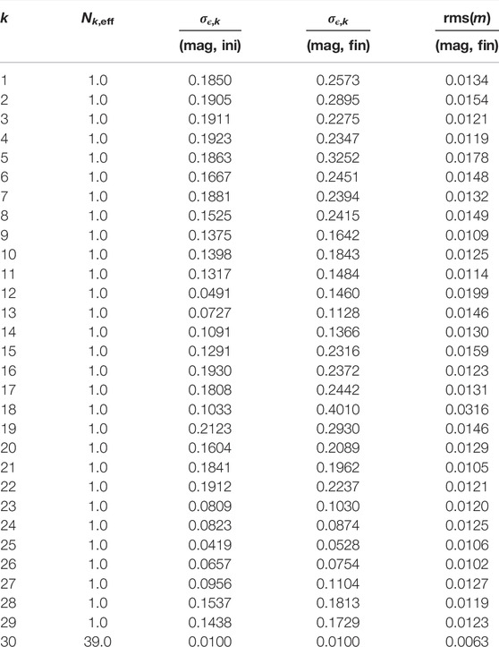
TABLE 7. As in Table 6 for the GS-asteroid in the case of absolute photometry with N_k,eff = 1 in Eq. 23.

Figure 9 shows examples of simulated lightcurves and the modeling results from MCMC sampling. The overall match between the simulated observations and modeling is quite satisfactory, but there are some systematics present, in particular, for the dense lightcurve #12 in the case of relative photometry. The conservative error model for absolute photometry shows up as large uncertainty envelopes using all of the MCMC samples, the standard deviations being significantly smaller.

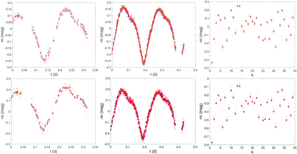
FIGURE 9. Example photometric lightcurves for the Gaussian-random-sphere asteroid (GS-asteroid). We show the dense photometric lightcurves #12 and #5 and the sparse lightcurve (blue circles; left, middle, and right, respectively; see Tables 5–7) together with the best-fit convex model lightcurves (red crosses) with 1-σ standard deviations (red bars) and uncertainty envelopes using all 30,000 Markov-chain Monte Carlo (MCMC) sample solutions (red points). We depict the results for relative (top) and absolute lightcurves (bottom). m, t, and k stand for relative magnitude, time from the first lightcurve observation, and lightcurve observation counter, respectively.

Table 8 gives the true rotational parameters used in the generation of the simulated data. Thereafter, it includes the results from least-squares and MCMC inversion, using ellipsoids and general convex shapes, for the rotational and phase function parameters in the cases of relative and absolute simulated data. Note that the angular width of the opposition effect has been assumed to be α₀ = 3° in the cases of absolute data. The reason is that the present data set has been insufficient to reliably predict the angular width. With the fixed value of α₀ = 3°, we have β_S (20°) ≈ β₀ + m₀ × 0.02431/rad from Eq. 9. For the absolute photometry, the mean values from MCMC sampling are β_S(20°) = 1.725 mag/rad using ellipsoid inversion and β_S(20°) = 1.670 mag/rad using convex inversion. Both values remain reasonably close to the corresponding values of β₀. Based on the H, G₁, G₂ fit to the lunar phase curve (Muinonen et al., 2010), the lunar photometric slope at 20° phase angle is 1.659 mag/rad. We obtain β_S(20°) = 2.06 ± 0.23, 1.825 ± 0.063, 1.725 ± 0.085, and 1.670 ± 0.041 in the cases of ellipsoid and convex inversion with relative data and ellipsoid and convex inversion with absolute data, respectively. With absolute photometry, both convex and ellipsoid inversion yield accurate results. For relative photometry, the retrieved slopes differ more substantially from the lunar slope. Based on the uncertainties, the lunar slope is, however, encompassed with reasonable probability.

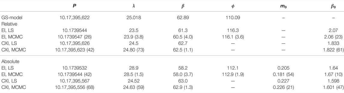
TABLE 8. Rotation period P (h), pole longitude λ (°) and latitude β (°), rotational phase ϕ (°), and phase-curve parameters m₀ (mag) and β₀ (mag/rad) for the simulated Gaussian-sphere asteroid. The parameter values on the topmost line (GS-model) represent those utilized to simulate the observations. For the simulation of the scattering model, see text. On the lines that follow, the parameter values represent least-squares solutions (LS) and means from MCMC sampling (MCMC) as obtained from ellipsoid inversion (EI) and convex inversion (CXI) in the cases of relative (Relative) and absolute simulated observations (Absolute). For the MCMC solutions, the parameter 1-σ standard deviations are given in the units of the last digit shown.

Table 9 gives the correlation coefficient for the rotational and phase function parameters, as computed from the MCMC samples. Considerable and realistic correlations are found for pole longitude and latitude and for m₀ and β₀ in the case of absolute photometry. In ellipsoid inversion, the rotational phase correlates with the pole longitude.

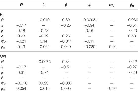
TABLE 9. Correlation coefficients for the rotation period P (h), pole longitude λ (°) and latitude β (°), rotational phase ϕ (°), and phase-curve parameters m₀ (mag) and β₀ (mag/rad) for MCMC lightcurve inversion using ellipsoids (EI for ellipsoid inversion) and convex shapes (CXI for convex inversion) in the case of the simulated GS asteroid. The upper (lower) triangles depict the coefficients in the case of relative (absolute) simulated observations.

It is clear that, with ellipsoids, there can be statistically significant differences from the true values of the parameters. However, with the current error modeling, ellipsoid inversion works in an acceptable way both for relative and absolute photometry. For more solid conclusions, additional examples must be studied. Convex inversion works well for both relative and absolute data.

Figures 10, 11 depict MCMC samples from convex inversion for the rotational and photometric parameters, and two spherical harmonics coefficients of the Gaussian surface density. Whereas the true rotation period is close to the centers of the distributions for relative photometry, there are apparent biases for absolute data. Since we have simulated the lightcurve data by using an advanced particulate medium scattering model, there are strictly no true values for the photometric parameters to compare with.

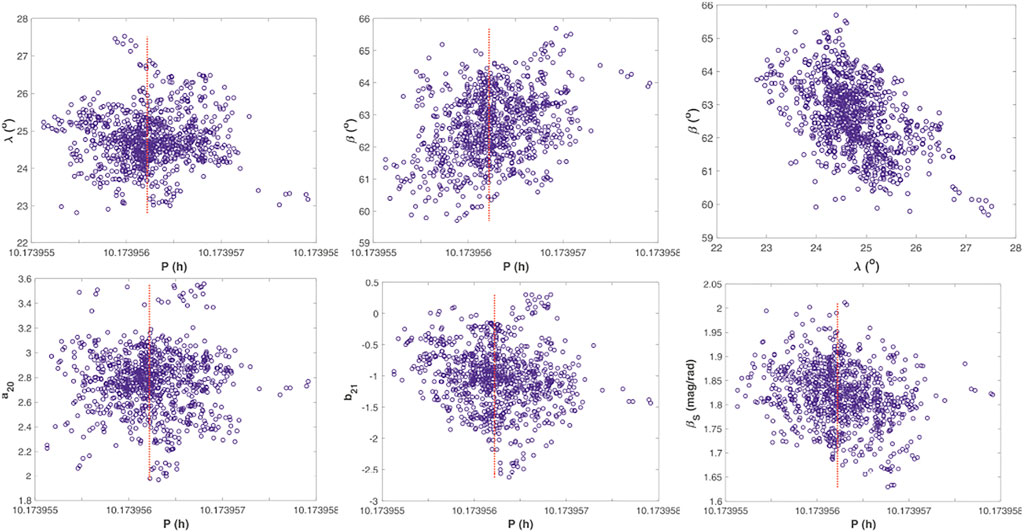
FIGURE 10. MCMC sampling of the rotational, shape, and photometric phase-curve parameters for the GS-asteroid simulation in the case of relative lightcurves. The marginal probabilitity densities are characterized by an unbiased sub-sample of 1,000 parameter sets selected from the complete sample of 30,000 sets. We depict rotational pole longitude (λ) and latitude (β) vs. rotation period (P; up to the left and middle, respectively), pole longitude vs. pole latitude (up to the right), example spherical harmonics coefficients a₂₀ and b₂₁ vs. rotation period (down to the left and middle, respectively), and photometric slope (β_S (20°)) vs. rotation period (down to the right). The red, dotted line marks the true rotation period.

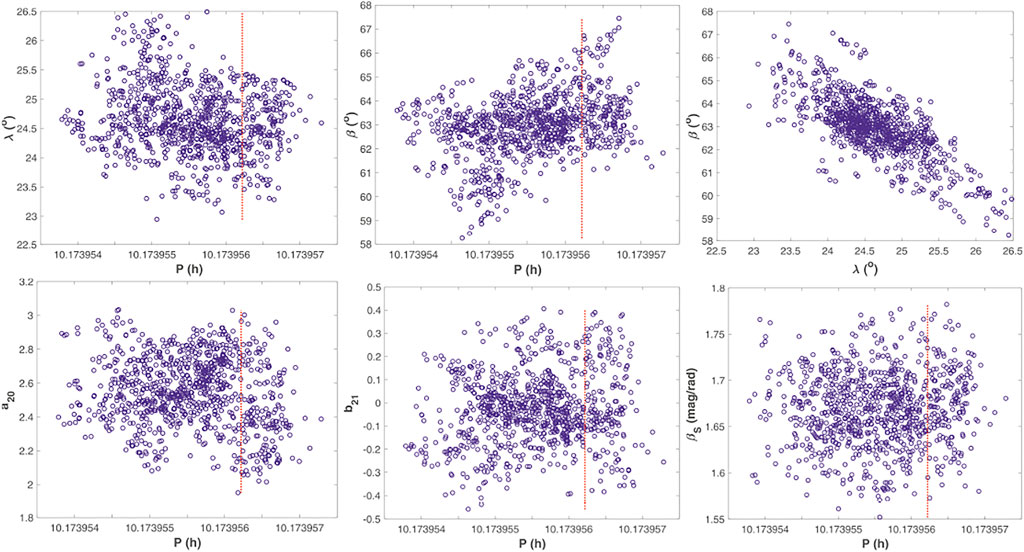
FIGURE 11. As in Figure 10 in the case of absolute photometry.

5 Conclusion

We have provided models of observational uncertainties for four classes of lightcurves, that is, for dense relative, sparse relative, dense absolute, and sparse absolute lightcurves. We have studied the models using an asteroid simulation based on the Gaussian-random-sphere shape model, making use of linear or linear-exponential phase function models for phase angles below 50° on the magnitude scale.

We have extended the Bayesian lightcurve inversion methods to allow for full retrieval of phase functions with their uncertainties and applied the methods to a set of some 500 asteroids with both ground-based and Gaia photometry. In comparison to earlier work, certain differences are seen in the mapping from apparent phase curves to intrinsic phase functions. These differences may derive, to an extent, from the scarce amount of Gaia DR2 photometry, and we expect to resolve the issues with the forthcoming Gaia DR3 photometry.

Finally, an asteroid’s spectrum from the ultraviolet (UV) through the visible (Vis) to the near-infrared (NIR) regime is known to vary with phase angle, evidently due to the fact that the phase function depends on the intrinsic brightness of the asteroid at a given wavelength. In the present work, we have confirmed that the shape and rotational parameters of the asteroid and the geometry of illumination and observation have an effect on the asteroid’s photometric phase function. The effect is different for different geometric albedos. Thus, the asteroid’s UV-Vis-NIR spectrum can depend on the shape and rotation parameters and vary as a function of the geometry of illumination and observation. It can be particularly enlightening to consider laboratory spectrometric measurements, such as those by Cloutis et al. (2012), extended to analogs of complete asteroids. The phase curve effects on the UV-Vis-NIR spectrometry and spectropolarimetry of asteroids remain as an open problem for future theoretical, observational, and experimental studies.

Data Availability Statement

The raw data supporting the conclusions of this article will be made available by the authors, without undue reservation.

Author Contributions

KM has been responsible for the article concept, programming, simulations, analysis, and writing the article. EU, together with JM, have contributed many of the figures. EU, JM, and AC have participated in writing the article and JM, AP, and XW have helped in the simulations and analysis. All have offered comments on the article.

Funding

Research supported by the Academy of Finland grants No. 1325805, No. 1336546, and No. 1345115, and the Chinese Academy of Sciences President’s International Fellowship Initiative (PIFI) Grant No. 2021VMA0017. This work presents results from the European Space Agency (ESA) space mission Gaia. Gaia data are being processed by the Gaia Data Processing and Analysis Consortium (DPAC). Funding for the DPAC is provided by national institutions, in particular the institutions participating in the Gaia MultiLateral Agreement (MLA). The Gaia mission website is https://www.cosmos.esa.int/gaia. The Gaia archive website is https://archives.esac.esa.int/gaia.

Conflict of Interest

The authors declare that the research was conducted in the absence of any commercial or financial relationships that could be construed as a potential conflict of interest.

The reviewer AC declared a past collaboration with the author AC to the handling editor.

Publisher’s Note

All claims expressed in this article are solely those of the authors and do not necessarily represent those of their affiliated organizations, or those of the publisher, the editors and the reviewers. Any product that may be evaluated in this article, or claim that may be made by its manufacturer, is not guaranteed or endorsed by the publisher.

References

Bowell, E. G., Hapke, B., Domingue, D., Lumme, K., Peltoniemi, J., and Harris, A. W. (1989). “Application of Photometric Models to Asteroids,” in Asteroids II. Editors T. Gehrels, M. T. Matthews, and R. P. Binzel (Tucson, Arizona, U.S.A.: University of Arizona Press), 524–555.
Cloutis, E. A., Hudon, P., Hiroi, T., Gaffey, M. J., Mann, P., and Bell, J. F. (2012). Spectral Reflectance Properties of Carbonaceous Chondrites: 6. Cv Chondrites. Icarus 221, 328–358. doi:10.1016/j.icarus.2012.07.007
Durech, J., Carry, B., Delbo, M., Kaasalainen, M., and Viikinkoski, M. (2015). “Asteroid Models from Multiple Data Sources,” in Asteroids IV. Editors P. Michel, F. E. DeMeo, and W. F. Bottke (Tucson, Arizona, U.S.A.: University of Arizona Press), 183–202. doi:10.2458/azu_uapress_9780816532131-ch010
Ďurech, J., Sidorin, V., and Kaasalainen, M. (2010). DAMIT: A Database of Asteroid Models. Astron. Astrophys. 513, A46. doi:10.1051/0004-6361/200912693
Farinella, P., Paolicchi, P., Tedesco, E. F., and Zappalà, V. (1981). Triaxial Equilibrium Ellipsoids Among the Asteroids? Icarus 46, 114–123. doi:10.1016/0019-1035(81)90081-6
Farinella, P., Paolicchi, P., and Zappalà, V. (1982). The Asteroids as Outcomes of Catastrophic Collisions. Icarus 52, 409–433. doi:10.1016/0019-1035(82)90003-3
Kaasalainen, M., Mottola, S., and Fulchignoni, M. (2002). “Asteroid Models from Disk-Integrated Data,” in Asteroids III. Editors W. Bottke, R. P. Binzel, A. Cellino, and P. Paolicchi (Tucson, Arizona, U.S.A.: University of Arizona Press), 139–150. doi:10.2307/j.ctv1v7zdn4.17
Kaasalainen, M., Torppa, J., and Muinonen, K. (2001). Optimization Methods for Asteroid Lightcurve Inversion: II. The Complete Inverse Problem. Icarus 153, 37–51. doi:10.1006/icar.2001.6674
Liddle, A. R. (2007). Information Criteria for Astrophysical Model Selection. Mon. Notices R. Astronomical Soc. Lett. 377, L74–L78. doi:10.1111/j.1745-3933.2007.00306.x
Lumme, K., and Bowell, E. (1981). Radiative Transfer in the Surfaces of Atmosphereless Bodies. I-Theory. II-Interpretation of Phase Curves. Astronomical J. 86, 1694–1704. doi:10.1086/113054
Magnusson, P., Barucci, M. A., Drummond, J. D., Lumme, K., Ostro, S. J., Surdej, J., et al. (1989). “Determination of Pole Orientations and Shapes of Asteroids,” in Asteroids II. Editors R. P. Binzel, T. Gehrels, and M. S. Matthews (Tucson, Arizona, U.S.A.: University of Arizona Press), 66–97.
Mahlke, M., Carry, B., and Denneau, L. (2021). Asteroid Phase Curves from Atlas Dual-Band Photometry. Icarus 354, 114094. doi:10.1016/j.icarus.2020.114094
Martikainen, J., Muinonen, K., Penttilä, A., Cellino, A., and Wang, X.-B. (2021). Asteroid Absolute Magnitudes and Phase Curve Parameters from Gaia Photometry. Astron. Astrophys. 649, A98. doi:10.1051/0004-6361/202039796
Muinonen, K., Belskaya, I. N., Cellino, A., Delbò, M., Levasseur-Regourd, A.-C., Penttilä, A., et al. (2010). A Three-Parameter Magnitude Phase Function for Asteroids. Icarus 209, 542–555. doi:10.1016/j.icarus.2010.04.003
Muinonen, K., and Lumme, K. (1991). “Light Scattering by Solar System Dust: the Opposition Effect and the Reversal of Linear Polarization,” in IAU Colloquium 126, Origin and Evolution of Dust in the Solar System, Kyoto, Japan, August 27–30, 1990. Editors A.-C. Levasseur-Regourd, and H. Hasekawa (Dordrecht, Netherlands: Kluwer Academic Publishers), 159–162. doi:10.1017/s0252921100066690
Muinonen, K., Parviainen, H., Näränen, J., Josset, J.-L., Beauvivre, S., Pinet, P., et al. (2011). Lunar Mare Single-Scattering, Porosity, and Surface-Roughness Properties with Smart-1 Amie. Astron. Astrophys. 531, A150. doi:10.1051/0004-6361/201016115
Muinonen, K., Piironen, J., Shkuratov, Y. G., Ovcharenko, A., and Clark, B. E. (2002). “Asteroid Photometric and Polarimetric Phase Effects,” in Asteroids III. Editors W. Bottke, R. P. Binzel, A. Cellino, and P. Paolicchi (Tucson, Arizona, U.S.A.: University of Arizona Press), 123–138. doi:10.2307/j.ctv1v7zdn4.16
Muinonen, K., Torppa, J., Wang, X.-B., Cellino, A., and Penttilä, A. (2020). Asteroid Lightcurve Inversion with Bayesian Inference. Astron. Astrophys. 642, A138. doi:10.1051/0004-6361/202038036
Muinonen, K., Wilkman, O., Cellino, A., Wang, X., and Wang, Y. (2015). Asteroid Lightcurve Inversion with Lommel-Seeliger Ellipsoids. Planet. Space Sci. 118, 227–241. doi:10.1016/j.pss.2015.09.005
Oszkiewicz, D. A., Muinonen, K., Bowell, E., Trilling, D., Penttilä, A., Pieniluoma, T., et al. (2011). Online Multi-Parameter Phase-Curve Fitting and Application to a Large Corpus of Asteroid Photometric Data. J. Quantitative Spectrosc. Radiat. Transf. 112, 1919–1929. doi:10.1016/j.jqsrt.2011.03.003
Penttilä, A., Shevchenko, V. G., Wilkman, O., and Muinonen, K. (2016). H, G1, G2 Photometric Phase Function Extended to Low-Accuracy Data. Planet. Space Sci. 123, 117–125. doi:10.1016/j.pss.2015.08.010
Shevchenko, V. G., Belskaya, I. N., Muinonen, K., Penttilä, A., Krugly, Y. N., Velichko, F. P., et al. (2016). Asteroid Observations at Low Phase Angles. IV. Average Parameters for the New H, G1, G2 Magnitude System. Planet. Space Sci. 123, 101–116. doi:10.1016/j.pss.2015.11.007
Gaia Collaboration Spoto, F., Tanga, P., Mignard, F., Berthier, J., Carry, B., et al. (2018). Gaia Data Release 2 Observations of Solar System Objects. Astron. Astrophys. 616, 24. doi:10.1051/0004-6361/201832900
Taylor, R. C. (1979). “Pole Orientation of Asteroids,” in Asteroids. Editors T. Gehrels, and M. S. Matthews (Tucson, Arizona, U.S.A.: University of Arizona Press), 480–493.
Torppa, J., and Muinonen, K. (2005). “Statistical Inversion of Gaia Photometry for Asteroid Spins and Shapes,” in Three-Dimensional Universe with Gaia. Editors C. Turon, K. S. O’Flaherty, and M. A. C. Perryman (Netherlands: ESA Publications Division ESTEC), 321–324. ESA Special Publications SP-576.
Wilkman, O., Muinonen, K., and Peltoniemi, J. (2015). Photometry of Dark Atmosphereless Planetary Bodies: an Efficient Numerical Model. Planet. Space Sci. 118, 250–255. doi:10.1016/j.pss.2015.06.004
Wilkman, O., Muinonen, K., Videen, G., Josset, J.-L., and Souchon, A. (2014). Lunar Photometric Modelling with Smart-1/amie Imaging Data. J. Quantitative Spectrosc. Radiat. Transf. 146, 529–539. doi:10.1016/j.jqsrt.2014.01.015
Keywords: asteroid, lightcurve, phase curve, phase function, absolute magnitude, convex inversion, asteroid taxonomy, Gaia mission
Citation: Muinonen K, Uvarova E, Martikainen J, Penttilä A, Cellino A and Wang X (2022) Asteroid Photometric Phase Functions From Bayesian Lightcurve Inversion. Front. Astron. Space Sci. 9:821125. doi: 10.3389/fspas.2022.821125
Received: 23 November 2021; Accepted: 23 May 2022;
Published: 17 June 2022.
Edited by:
Aaron Golden, National University of Ireland Galway, IrelandReviewed by:
Josep M. Trigo-Rodríguez, Institute of Space Sciences (CSIC), SpainApostolos Christou, Armagh Observatory, United Kingdom
Copyright © 2022 Muinonen, Uvarova, Martikainen, Penttilä, Cellino and Wang. This is an open-access article distributed under the terms of the Creative Commons Attribution License (CC BY). The use, distribution or reproduction in other forums is permitted, provided the original author(s) and the copyright owner(s) are credited and that the original publication in this journal is cited, in accordance with accepted academic practice. No use, distribution or reproduction is permitted which does not comply with these terms.
*Correspondence: Karri Muinonen, karri.muinonen@helsinki.fi