Observations of Pole-to-Pole, Stratosphere-to-Ionosphere Connection

Introduction

As the Earth’s ionosphere—the charged portion of the atmosphere with maximum ionization at ∼300 km—is created primarily by solar ionizing flux, conventional thinking implies that major variations in ionospheric electron density are related to solar and geomagnetic activity. While these factors are the primary drivers of ionospheric variability, many studies demonstrate significant variations in electron density due to the influences from the lower atmosphere through effects of gravity waves (Fritts and Lund, 2011, and references therein), tides (England, 2011, and references therein), and planetary waves (Pancheva and Mukhtarov, 2011). Terrestrial influences on ionospheric variability are often thought to be limited to a narrow geographic region or a short time frame. In the last decade it has become widely accepted that large (50–100% deviations from the background), persistent (>2 weeks) ionospheric variations are driven by middle atmosphere changes that are particularly enhanced during dramatic meteorological events called sudden stratospheric warmings (SSWs) (e.g., Goncharenko et al., 2010, 2021; Chau et al., 2012). SSWs cause large-scale variations in temperature, wind, and ozone density in the Arctic wintertime stratosphere at high latitudes (60–90°N). SSW-induced variations extend both above and below the stratosphere, and across the equator to the tropics and summer polar mesosphere (e.g., Karlsson et al., 2007, 2009; Smith et al., 2020), and to the tropical ionosphere (e.g., Pedatella et al., 2018). However, known ionospheric disturbances associated with such changes are believed to be greatest at low latitudes (0–20°) and to fall off rapidly in the mid-latitudes (Pancheva and Mukhtarov, 2011), implying complex mechanisms of atmospheric connections in both the vertical and horizontal directions.

The Earth’s ionosphere has been monitored for several decades, mostly by ionosondes due to their simplicity (Reinisch, 1986); however, such instruments allow studies of only local conditions. For the last 2 decades, large progress in understanding the spatial and temporal evolution of the ionosphere was achieved through observations of Total Electron Content (TEC) by ground-based Global Navigation Satellite System (GNSS) receivers. Although thousands of GNSS receivers are currently used in ionospheric research, data gaps over the oceans and hard-to-reach areas impact the utility of GNSS TEC data and hinder understanding of ionospheric behavior over those regions. Current knowledge of ionospheric physics is heavily influenced by observational data in the northern hemisphere, while the ionosphere above the sparsely instrumented southern hemisphere remains less understood. The last several years have seen an important development with the installation of new instrumentation in South America and Antarctica, enabling fundamentally new types of studies. This is the first work to leverage new instrumentation in South America and Antarctica to show that ionospheric variations at the summer high latitudes may be attributed to SSW. This study presents observations from independent techniques that show large-scale mesospheric and ionospheric variations in response to the Arctic SSW in January 2013. These variations occur not only at low latitudes, but at the middle latitudes and polar latitudes of the southern (opposite) hemisphere. The interhemispheric coupling mechanism (IHC, Becker et al., 2004) was invoked by de Wit et al. (2015) to explain variability at the summer polar mesopause during January 2013. Here we forge new territory by showing SSW-induced variability in the summer polar ionosphere.

Data and Methods

This work requires the use of disparate data to study pole-to-pole teleconnections between the winter stratosphere and summer ionosphere during January 2013. We use temperature measurements from the Aura Microwave Limb Sounder (MLS) (Waters et al., 2006) to determine the response of the middle atmosphere to the SSW 2013 event. Temperature anomalies are computed by removing the 2004–2021 average from each day; however, this average does not include the day in question.

Polar mesospheric cloud (PMC) frequencies are derived from measurements made by the Cloud Imaging and Particle Size (CIPS) instrument (McClintock et al., 2009), which is a nadir-viewing panoramic imager that measures scattered radiation at 265 nm. CIPS was launched in 2007 aboard the Aeronomy of Ice in the Mesosphere (AIM) satellite (Russell et al., 2009), and is still operational. CIPS is a nadir-viewing panoramic imager that measures scattered radiation at 265 nm. It provides high resolution images of PMC albedo near the summer polar mesopause every day over the entire summer polar cap (Lumpe et al., 2013). This work uses the v5.20r05 level 3c data, which has a spatial resolution of 56 km².

To determine characteristics of ionospheric disturbances, we employ global TEC maps that utilize ground-based vertical TEC values (measured with TEC unit TECU; one TECU = 10¹⁶ e⁻/m²) from several thousand GNSS receivers. The resolution of this data is 1°longitude by 1°latitude every 5 min. This work uses 17 years of data from 2000–2016. On each day, all TEC data in the American sector (75°W ± 7.5°) is averaged in 1°latitude by 1-h local time bins. To separate effects of meteorological or other types of forcing from known effects of solar, geomagnetic activity, and seasonal variations, we use an empirical model of TEC based on the same 17 years of data. See Goncharenko et al. (2018) for details on model formulation and performance. We construct the TEC model for 75°W by fitting each latitude and local time bin with a formula that combines a dependence on the F10.7 solar flux proxy, a dependence on the Ap geomagnetic activity index and its history, a sinusoidal parameterization of seasonal variation, and a modulation of seasonal variations by solar activity. Fitting coefficients are obtained independently for every 1°latitude and 1-h local time bin, thus avoiding artificial features that can be introduced by fitting with 24-, 12-, and 8-h tides. Subtracting empirical model estimates from the observational data produces residuals that we interpret as having a meteorological origin. Note that inclusion of additional terms in the fit formula does not change the residuals significantly and does not change the results of this study. The TEC model was developed only for 75°W due to the relative data scarcity at other longitudes; however, this approach can be applied in the future to other locations as more data for a variety of conditions becomes available.

For comparison with TEC results, we have analyzed ionosonde data on maximum F-region density (NmF2) that is highly correlated with TEC. We used data from two instruments that are located in the American longitudinal sector, the Port Stanley (51.6°S, 57.9°W) digisonde and the Vernadsky (65.1°S, 64.2°W) ionosonde. The Port Stanley digisonde data was provided by the Lowell GIRO Data Center (http://spase.info/VWO/NumericalData/GIRO/CHARS.PT15M) which is discussed by Reinisch and Galkin (2011). The Vernadsky ionosonde data is provided by the National Antarctic Scientific Center of Ukraine, which has operated Vernadsky station since 1996. We use Port Stanley data collected in 1997–2015 and Vernadsky data collected in 2011–2013 to construct empirical models of NmF2 in the same manner as described above for GNSS TEC.

Results

In January 2013, a major Arctic SSW caused significant disturbances in Earth’s middle atmosphere. Figure 1A (top panel) shows the temperature impacts, using MLS satellite observations. This major SSW was associated with the growth of planetary wave-2, which split the stratospheric polar vortex. As is typical for SSWs, the momentum deposited by the planetary wave breaking altered the mesospheric residual circulation, leading to anomalous descent and warming in the polar winter stratosphere and upwelling and cooling in the polar winter mesosphere, as indicated in Figure 1A. Stratospheric polar temperatures maximized on January 11th and mesospheric cooling peaked on January 12th.

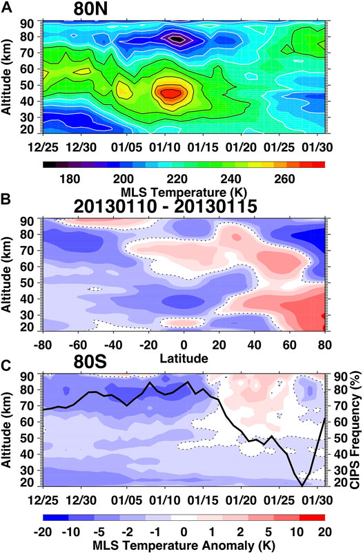
FIGURE 1. (A) Altitude-time section of zonal mean MLS temperature averaged at 80°N from December 25, 2012 through January 31, 2013, (B) Latitude-altitude section of zonal mean temperature anomalies (deviations from the time mean) averaged from 10 to 15 January 2013, (C) Altitude-time section of temperature anomalies at 80° S from December 25, 2012 through January 31, 2013. The thick black line indicates daily CIPS PMC frequencies (number of pixels in which a PMC was detected relative to the total number of pixels, in %) at 80°S for clouds with albedos greater than 5 × 10^–6 sr⁻¹, smoothed over 3 days.

The teleconnection pattern whereby planetary wave disturbances in the winter stratosphere lead to temperature variations at the summer mesopause is referred to as interhemispheric coupling (IHC) (e.g., Becker and Schmitz, 2003; Becker et al., 2004; Becker and Fritts, 2006; Karlsson et al., 2007; 2009). Figure 1B shows 5-days average temperature anomalies for 10–15 January, during the peak SSW and mesospheric cooling. The classic quadrupole pattern in temperature anomalies is in an agreement with de Wit et al. (2015) (Figure 4), who documented IHC coupling during the same SSW. This panel illustrates the low latitude and summer hemisphere extension of SSW-induced temperature perturbations. Several IHC mechanisms are described as follows. The cooling in the tropical stratosphere and warming in the tropical mesosphere causes meridional temperature gradients (and thus zonal winds) in the summer hemisphere to strengthen. The tropical warm anomaly in the mesosphere (red area in Figure 1B) increases the summer hemisphere equator-to-pole temperature gradient, leading to a westerly shift in the zonal winds in the summer upper mesosphere. According to Körnich and Becker (2010), this causes a lowering of the zero wind line, and thus a lowering of the altitude at which gravity waves break. The resulting downward shift in the ascending branch of the residual circulation then leads to warming near the summer polar mesopause. Smith et al. (2020) found repeatable temperature correlations between the winter stratosphere and the summer mesopause that exhibited expected IHC latitude-altitude structures (Randel, 1993) in 195 simulated years in the Whole Atmosphere Community Climate Model; however, they could not confirm that gravity wave filtering was the primary coupling mechanism in the model. Rather, they concluded that IHC in the model is due to a compensating circulation that arises to restore balance to the zonal mean atmosphere. Further, France et al. (2018) and Lieberman et al. (2021) showed that warming at the summer mesopause can arise due to inertial instability-triggered growth of the quasi-2-days wave. Thus, while IHC is both observed and simulated, the mechanisms responsible for the coupling remain elusive.

Figure 1C shows the time evolution of temperature anomalies in the stratosphere and mesosphere of the summer hemisphere. Prior to the SSW, the summer mesosphere was significantly colder than average, as evidenced by the persistent negative anomalies above ∼60 km over the southern polar cap in late December and early January. However, within days of the SSW, the negative temperature anomalies decreased in magnitude and then turned positive. This is due to warming in the polar summer mesosphere; this warming is consistent with a sharp decrease in PMC frequencies (given by the thick black line). The changes in Antarctic summer mesopause temperatures and PMC frequencies are consistent with robust IHC processes.

To understand ionospheric behavior during this period, we focus on GNSS TEC in the American longitudinal sector, where evolution of TEC with latitude can be investigated in detail due to the dense network of GNSS receivers. Large, long-lasting ionospheric disturbances in response to this SSW event were reported in earlier studies at low latitudes and peaked in mid-January (Goncharenko et al., 2013; Jonah et al., 2014). Figure 2A shows the latitudinal variation in the TEC anomaly at 75°W on January 16, 2013, a geomagnetically quiet day (Ap = 5) during moderate solar activity (F10.7 = 137). The TEC anomaly is calculated as a difference between TEC observations and expected TEC behavior, which is provided by the empirical TEC model described in Data and Methods and in Goncharenko et al. (2018). The anomaly in TEC (Figure 2A) includes a large increase in the northern crest of the Equatorial Ionization Anomaly (EIA, 0–15°N) in the morning-noon sector (12–18 UT) and a decrease in the afternoon and evening sectors (21–3 UT), as was reported for multiple SSW events in numerous studies (see reviews Chau et al., 2012; Goncharenko et al., 2021).

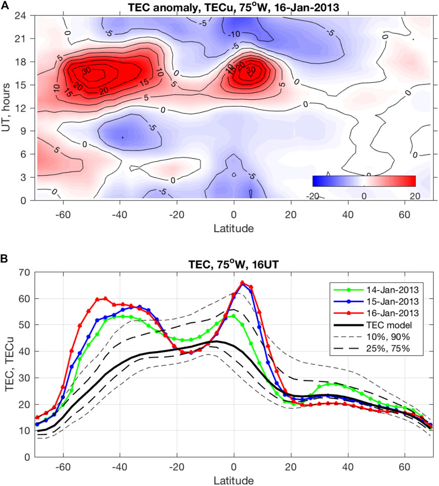
FIGURE 2. (A) Anomaly in the total electron content at 75°W on Jan 16, 2013 extends from equatorial to high latitudes of the southern hemisphere. (B) TEC variation with latitude for 75°W and 16 UT (11 AM Local Time). Shown are TEC values observed on January 14–16, 2013 (green, blue, red) compared with TEC values expected for this season and solar activity as predicted by the empirical model (black). Thick dash lines show 25th and 75th percentiles of all available data, thin dash lines show 10th and 90th percentiles. Percentiles were calculated using TEC observations with close solar flux conditions (127 < F10.7 < 136) and from mid-December to mid-February.

Observations in January 2013 show that an even larger morning-noon TEC anomaly develops in the southern hemisphere, centered at 40–60°S and extending to high latitudes, as seen in Figure 2A. Figure 2B shows the latitudinal variation in TEC at 16 UT (11:00 AM local time) for three consecutive geomagnetically quiet days, 14–16 January 2013; similar TEC variations are observed over the 10-days period. Continuous extension of TEC anomalies up to a factor of two from the expected value is observed from ∼20°S all the way to the high latitudes in the southern hemisphere. Recent modeling studies are coming to a consensus that amplification in solar and lunar semidiurnal tides during SSWs is the most likely physical mechanism driving variations in the electric field and plasma velocity at the magnetic equator and, consequently, in plasma density in the EIA region (Fang et al., 2012; Jin et al., 2012; Pedatella and Liu, 2013; Wang et al., 2014). Solar semidiurnal migrating tides (SW2) experience stronger amplifications in the mid-latitude southern hemisphere than in the northern hemisphere (Liu et al., 2010). Upward propagation of these tides can modulate the thermospheric wind system and directly influence the ionosphere, particularly at middle latitudes. Pedatella and Maute (2015) also suggest that semidiurnal lunar tides amplified during SSWs propagate all the way to the upper thermosphere, leading to the quasi-semidiurnal variation of the F-region peak height and, consequently, electron density. As lunar tides were strongly amplified during the 2013 SSW (Zhang and Forbes, 2014), our observations of increased TEC at southern hemisphere mid-latitudes support both solar and lunar semidiurnal tide mechanisms.

In addition to the morning-noon enhancement, nighttime (3-8 UT) electron density is also enhanced at latitudes higher than ∼45°S (Figure 2A); for example, the ionospheric Weddell Sea Anomaly, a phenomenon when the nighttime electron density exceeds the daytime electron density (Penndorf, 1965; He et al., 2009), is modified during both nighttime and daytime hours, as seen in Figure 2A at 60–70°S. We note that Figure 2 extends only to 70°S, as empirical TEC model did not include higher latitudes due to the data scarcity. Figure 3 further illustrates extension of the observed ionospheric anomalies to the high latitudes in the southern hemisphere, up to the South Pole. Polar maps compare TEC distributions on January 15, 2012, an undisturbed Arctic winter day the previous year (panels (3A) and (3B), to January 16, 2013, a SSW day (panels 3C and 3D). The control day of January 15, 2012 was chosen to minimize differences due to seasonal change, solar flux, and geomagnetic activity (F10.7 = 133, Ap = 4 on Jan 15, 2012; F10.7 = 137, Ap = 5 on Jan 16, 2013). The TEC increase on January 16, 2013 (SSW day) at 4 UT is observed over the entire Antarctic continent, as seen in Figure 3C. The largest enhancements are over the Antarctic Peninsula and the Weddell Sea in the western hemisphere and near the Antarctic coast and 90°E. At 15 UT (Figure 3D), increases in TEC over the Antarctic Peninsula and the Weddell Sea are clearly an extension of the TEC change that peaked in the middle latitudes of the southern hemisphere, as shown in Figures 2A,B. Ionospheric disturbances similar to those presented in Figures 3C,D were observed for several days and maximized on January 14–16, 2013, simultaneously with disturbances at lower latitudes seen in Figure 2.

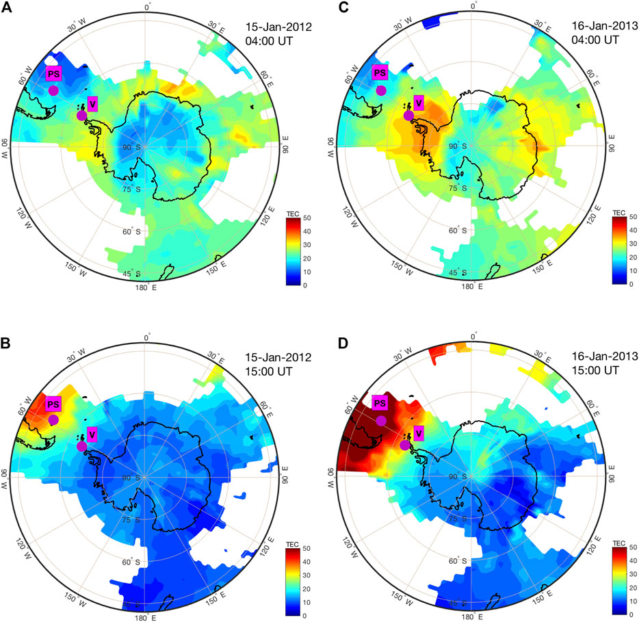
FIGURE 3. Southern hemisphere polar maps showing TEC behavior during undisturbed Arctic conditions in January 2012 (left side, A, B) and during an SSW in January 2013 (right side, C, D). Top panels show snapshots at 4:00 UT and demonstrate increases in TEC over the entire Antarctic continent, with particularly large enhancement around the Antarctic Peninsula (30–120°W). Bottom panels (snapshots at 15:00 UT) demonstrate a strong increase in TEC from ∼60°E to 120°W, with largest increases in the American longitudinal sector. Magenta dots indicate the locations of the Port Stanley and Vernadsky ionosondes stations.

Independent confirmation of the impact of an Arctic SSW on the ionosphere over the middle and high latitudes of southern hemisphere is further obtained using a different observational technique, namely ionosondes. Figure 4 shows diurnal variations in the peak electron density NmF2 at mid- and high-latitude stations: Port Stanley (51.6°S, 57.9°W) and Vernadsky (65.1°S, 64.2°W), respectively. Typical diurnal variations of NmF2 (black lines) at these locations are very different. Daytime NmF2 (at ∼12–18 UT) over Port Stanley (Figure 4A) exceeds nighttime NmF2 (at ∼1-6 UT) by ∼50–60%, as expected in the mid-latitude summer hemisphere, consistent with effects of maximum photo-ionization rates at noon due to the smallest solar zenith angle and indicating that solar photoionization is the dominant mechanism responsible for NmF2 behavior. In contrast to middle latitude, at high latitude over the Vernadsky location (Figure 4B) nighttime NmF2 exceeds daytime NmF2 by a factor of ∼2, as expected for the area of the Weddell Sea Anomaly. This behavior in typical NmF2 indicates significant contributions to NmF2 from ionospheric dynamics, including thermospheric neutral wind and E x B drift, and from composition (Chen et al., 2011; Richards et al., 2017). During the SSW, similar ionospheric anomalies are observed at both locations: dramatic increases (up to a factor of 2) in NmF2 during daytime hours (∼12–18 UT), weaker increases at night (1-6 UT), and a slight decrease in the morning hours (6-9 UT). These anomalies are fully consistent with the GNSS TEC observations shown in Figures 2, 3. The similarity of the diurnal behavior in ionospheric anomalies in the geographic mid- and high-latitude southern hemisphere suggest that they could be driven by the same mechanism, despite very different mechanisms being responsible for the typical/climatological ionospheric behavior in these regions. Seasonal variations in the meridional wind have long been considered an important driver of the Weddell Sea Anomaly (Jee et al., 2009). Thus, we suggest that SSW-associated semidiurnal variations in the upper thermospheric wind system is likely a leading mechanism responsible for large ionospheric disturbances in the high-latitude southern hemisphere during this SSW event.

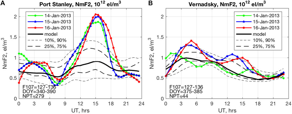
FIGURE 4. Variations in the peak electron density NmF2 as measured by ionosondes at Port Stanley (A) and Vernadsky (B). Highly anomalous increases in NmF2 are observed at both locations during the SSW, as illustrated with data from January 14–16, 2013.

Discussion

Our observations demonstrate that during the 2013 Arctic SSW event, an extended region of atmospheric anomalies formed in the southern hemisphere. This region spans the mesosphere (60–90 km) to the ionosphere (∼100–1,000 km) and from summer mid-latitudes to the South Pole, and persists for days. The formation of mesospheric and ionospheric anomalies in the mid- and high-latitude southern hemisphere during the northern hemisphere winter SSW presents a fascinating example of atmospheric coupling that is most likely driven by multiple mechanisms. Although we do not fully understand how the Arctic SSW leads to the ionospheric variability in the summer hemisphere, the following discussion presents some hypotheses about associated mechanisms. These hypotheses need to be tested with both additional observations and numerical simulations.

In the mesosphere, warming of the summer mesopause region in late January 2013 and associated decrease in the frequency of PMCs has been attributed to IHC. The notion that large planetary wave activity and warming in the polar winter stratosphere is correlated with increasing temperatures at the polar summer mesopause is well accepted. However, as explained above, several mechanisms have been proposed to explain this global teleconnection. It is still unclear whether one or more of these mechanisms are at play in different situations. The weakened ascent near the summer mesopause due to IHC is also consistent with the SSW-induced weakening of the residual circulation in the lower thermosphere reported by Miyoshi et al. (2015).

In the ionosphere, the formation of anomalous features over the entire Antarctic continent likely results from thermospheric wind changes brought about by the SSW. At thermospheric altitudes, the wind changes could result from the superposition of migrating semidiurnal solar tides (SW2), non-migrating solar semidiurnal tides (SW1), and semidiurnal lunar tides (M1, M2). Enhancement of the SW2 tide during SSWs is a well-known phenomenon documented in both observations and simulations (Liu et al., 2010; Pedatella and Liu, 2013; Limpasuvan et al., 2016). The SW1 tide is generated through interaction of planetary wave 1 with solar semidiurnal migrating tide SW2. Simulations by Liu et al. (2010) indicate that amplitudes of the resulting SW1 tide in the meridional wind are larger in the mid-latitude southern hemisphere than in the northern hemisphere, and are particularly strongly enhanced in the high-latitude southern hemisphere. The SW1 tide remains strong even in the high-latitude upper thermosphere, making it potentially a key component for ionospheric variability above Antarctica. The semidiurnal lunar tide was particularly strongly amplified during the January 2013 SSW, as reported by Zhang and Forbes (2014). Liu et al. (2021) found that lunar tides in ionospheric TEC are not symmetric in latitude in several cases of analyzed SSW events, and signatures of lunar tides extend deep into middle latitudes of the southern hemisphere and weaken the Weddell Sea Anomaly. We thus can expect that amplification of any of the above-mentioned tides in association with SSWs can influence thermospheric winds at middle to high latitudes in the southern hemisphere. Superposition of these tidal components (SW2, SW1, M1, M2) of varying amplitudes and phases creates a complicated pattern of anomalies in the thermospheric wind and, consequently, in the ionosphere above Antarctica.

Additionally, Miyoshi et al. (2015) found that the effect of a winter SSW is to weaken the summer residual circulation between ∼80 and ∼400 km, including decreased descent in the summer polar lower thermosphere and weakened ascent above ∼120 km. These thermospheric circulation changes are compounded with IHC effects to weaken ascent near the summer mesopause. In general, upwelling decreases the O/N₂ ratio and tends to decrease ionospheric electron density (e.g., Rishbeth, 1998). Weaker upwelling in the upper thermosphere at high latitudes of the southern hemisphere predicted by Miyoshi et al. (2015) would result in a higher thermospheric O/N₂ ratio and contribute to an overall increase in ionospheric electron density and TEC observed over Antarctica. Such an increase is seen in Figure 2A as a general enhancement in TEC at 60–70°S, which is observed in addition to the quasi-semidiurnal variation discussed above. An increase in TEC at even higher latitudes, including the overall increase in TEC above Antarctica seen in Figure 3C, might also be linked to SSW-induced variations in thermospheric composition. Pedatella et al. (2016) reveled a slight increase in O/N₂ at high latitudes of the southern hemisphere in TIE-GCM simulations and in COSMIC zonal mean peak electron density during the SSW of January 2009. Although their study was limited to lower latitudes than Antarctica, it is consistent with the general increase in TEC above Antarctica reported here. We note that SSW-induced changes in the thermospheric composition can vary strongly with latitude, as they are driven by variations in thermospheric circulation. Other simulations emphasized changes in thermospheric composition [such as (O), (O₂), (N₂), (H)] induced by the dissipation of amplified tides and generally predicted a decrease in the O/N₂ ratio at low and middle latitudes that would lead to a decrease in ionospheric electron density and TEC (Yamazaki and Richmond, 2013; Pedatella et al., 2016; Jones et al., 2020). The topic of changes in composition of different species has not been explored yet with sufficient detail and requires additional observational and modeling effort.

We cannot rule out the influence on ionospheric electron density that is produced by electric fields; these effects contribute significantly to the vertical plasma motion in the low-latitude ionosphere and are a well-known driver of the EIA (Anderson, 1981). Usually, effects of the electric field are not expected to contribute significantly to variations in electron density at middle and high latitudes, due to the high inclination angle of the Earth’s magnetic field lines closer to its poles. However, the inclination angle at high latitudes in the southern hemisphere (58 at Vernadsky) is smaller than in the northern hemisphere (for American longitudes), and an electric field can produce non-negligible electron density variations. Numerical simulations demonstrate that significant perturbations in the mid-to-high latitude F-region vertical ion drift can be generated by inclusion of planetary waves at the model’s lower boundary (Liu et al., 2010).

Conclusion

This study investigated the behavior of the mesosphere and ionosphere at geographic high latitudes of the southern hemisphere during and after the Arctic SSW of January 2013. We use a combination of stratospheric, mesospheric, and ionospheric ground-based and satellite data to demonstrate anomalous behavior in multiple parameters during a multi-day period in January 2013—neutral temperature, PMC frequency, TEC, and peak electron density. Our observations show that persistent mesospheric and ionospheric anomalies that are observed above Antarctica in January 2013 may be related to the SSW in the Arctic stratosphere. The results provide strong observational evidence that SSW events generate truly global disturbances that reach the high latitudes of the opposite hemisphere; thus, this study extends the concept of inter-hemispheric coupling to polar ionosphere. A variety of mechanisms is proposed to interpret the observed atmospheric and ionospheric variations at middle and high latitudes in the southern hemisphere, but their relative importance is not known yet. This paper aims to spark curiosity and encourage the scientific community to quantify the contributions of the different mechanisms proposed here, and to suggest or consider other mechanisms responsible for the mesospheric and ionospheric variability seen in the observations. Continuous, high-quality observations of mesospheric, thermospheric and ionospheric parameters are critical for the robust identification of essential features. As the southern hemisphere remains poorly instrumented, detailed studies of this coupling remain a matter of future research.

Data Availability Statement

Publicly available datasets were analyzed in this study. This data can be found here: MLS satellite data is available via http://mls.jpl.nasa.gov/. GNSS TEC data are publicly available through the CEDAR Madrigal database at http://cedar.openmadrigal.org. The Port Stanley digisonde data is available at http://giro.uml.edu/. Data obtained by Vernadsky ionosonde is available at http://geospace.com.ua/databrowser.

Author Contributions

LPG: all aspects of paper; VLH and CER: analysis and interpretation of MLS and CIPS data; S-RZ: interpretation of ionospheric data; AJC: TEC data coordination and interpretation; AZ and IG: ionosonde data coordination and interpretation; MS: TEC data processing.

Funding

Research and operations at MIT Haystack Observatory are supported by the cooperative agreement AGS-1952737 between the US National Science Foundation and the Massachusetts Institute of Technology. LPG was also supported by the NASA grant 80NSSC19K0262 and NSF grant AGS-1132267. VLH was supported by the NASA grants 80NSSC18K1046 and 80NSSC20K0628. CER was supported by the NASA Small Explorer Program through contract # NAS5-03132. CER and VLH were also supported by the NASA grant 80NSSC20K0628. SZ was supported by the AFOSR FA9559-16-1-0364. AZ is partially supported through EOARD-STCU- IRA NASU Partner projects P667 and P735. MS was supported by the Research Experience for Undergraduates grant for her internship at MIT Haystack Observatory.

Conflict of Interest

The authors declare that the research was conducted in the absence of any commercial or financial relationships that could be construed as a potential conflict of interest.

Publisher’s Note

All claims expressed in this article are solely those of the authors and do not necessarily represent those of their affiliated organizations, or those of the publisher, the editors and the reviewers. Any product that may be evaluated in this article, or claim that may be made by its manufacturer, is not guaranteed or endorsed by the publisher.

Acknowledgments

We thank the MLS science team for processing and freely distributing the satellite data via http://mls.jpl.nasa.gov/. GNSS TEC data are publicly available through the CEDAR Madrigal database at http://cedar.openmadrigal.org. We thank the operators of the digisonde at Port Stanley (United Kingdom) for sharing their data through http://giro.uml.edu/. Data obtained by Vernadsky ionosonde is available at http://geospace.com.ua/databrowser.

References

Anderson, D. N. (1981). Modeling the Ambient, Low Latitude F-Region Ionosphere-A Review. J. Atmos. Terrestrial Phys. 43, 753–762. doi:10.1016/0021-9169(81)90051-9
Becker, E., and Fritts, D. C. (2006). Enhanced Gravity-Wave Activity and Interhemispheric Coupling during the MacWAVE/MIDAS Northern Summer Program 2002. Ann. Geophys. 24, 1175–1188. doi:10.5194/angeo-24-1175-2006
Becker, E., Müllemann, A., Lübken, F.-J., Körnich, H., Hoffmann, P., and Rapp, M. (2004). High Rossby-Wave Activity in Austral winter 2002: Modulation of the General Circulation of the MLT during the MaCWAVE/MIDAS Northern Summer Program. Geophys. Res. Lett. 31, L24S03. doi:10.1029/2004GL019615
Becker, E., and Schmitz, G. (2003). Climatological Effects of Orography and Land-Sea Heating Contrasts on the Gravity Wave-Driven Circulation of the Mesosphere. J. Atmos. Sci. 60, 103–118. doi:10.1175/1520-0469(2003)060<0103:ceooal>2.0.co;2
Chau, J. L., Goncharenko, L. P., Fejer, B. G., and Liu, H.-L. (2012). Equatorial and Low Latitude Ionospheric Effects during Sudden Stratospheric Warming Events. Space Sci. Rev. 168, 385–417. doi:10.1007/s11214-011-9797-5
Chen, C. H., Huba, J. D., Saito, A., Lin, C. H., and Liu, J. Y. (2011). Theoretical Study of the Ionospheric Weddell Sea Anomaly Using Sami2. J. Geophys. Res. 116, a–n. doi:10.1029/2010JA015573
de Wit, R. J., Hibbins, R. E., Espy, P. J., and Hennum, E. A. (2015). Coupling in the Middle Atmosphere Related to the 2013 Major Sudden Stratospheric Warming. Ann. Geophys. 33, 309–319. doi:10.5194/angeo-33-309-2015
England, S. L. (2011). A Review of the Effects of Non-migrating Atmospheric Tides on the Earth's Low-Latitude Ionosphere. Space Sci. Rev. 168, 211–236. doi:10.1007/s11214-011-9842-4
Fang, T.-W., Fuller-Rowell, T., Akmaev, R., Wu, F., Wang, H., and Anderson, D. (2012). Longitudinal Variation of Ionospheric Vertical Drifts during the 2009 Sudden Stratospheric Warming. J. Geophys. Res. 117, A03324. doi:10.1029/2011JA017348
France, J. A., Randall, C. E., Lieberman, R. S., Harvey, V. L., Eckermann, S. D., Siskind, D. E., et al. (2018). Local and Remote Planetary Wave Effects on Polar Mesospheric Clouds in the Northern Hemisphere in 2014. J. Geophys. Res. Atmos. 123, 5149–5162. doi:10.1029/2017JD028224
Fritts, D. C., and Lund, T. S. (2011). “Gravity Wave Influences in the Thermosphere and Ionosphere: Observations and Recent Modeling,” in A. Bhattacharyya (Coed.), Aeronomy of the Earth’s Atmosphere and Ionosphere, IAGA Special Sopron Book Series 2. Editors M. A. Abdu, and D. Pancheva (© Springer Science+Business Media B.V), 109–130. doi:10.1007/978-94-007-0326-1_8
Goncharenko, L., Chau, J. L., Condor, P., Coster, A., and Benkevitch, L. (2013). Ionospheric Effects of Sudden Stratospheric Warming during Moderate-To-High Solar Activity: Case Study of January 2013. Geophys. Res. Lett. 40, 4982–4986. doi:10.1002/grl.50980
Goncharenko, L., Harvey, V., Liu, H., and Pedatella, N. (2021). “Sudden Stratospheric Warming Impacts on the Ionosphere‐thermosphere System—A Review of Recent Progress,”. Space Physics and Aeronomy: Advances in Ionospheric Research: Current Understanding and Challenges. Editors C. Huang, and G. Lu (Hoboken, NJ: Wiley), Vol. 3.
Goncharenko, L. P., Chau, J. L., Liu, H.-L., and Coster, A. J. (2010). Unexpected Connections between the Stratosphere and Ionosphere. Geophys. Res. Lett. 37. doi:10.1029/2010GL043125
Goncharenko, L. P., Coster, A. J., Zhang, S. R., Erickson, P. J., Benkevitch, L., Aponte, N., et al. (2018). Deep Ionospheric Hole Created by Sudden Stratospheric Warming in the Nighttime Ionosphere. J. Geophys. Res. Space Phys. 123, 7621–7633. doi:10.1029/2018JA025541
He, M., Liu, L., Wan, W., Ning, B., Zhao, B., Wen, J., et al. (2009). A Study of the Weddell Sea Anomaly Observed by FORMOSAT-3/COSMIC. J. Geophys. Res. 114 (A12). doi:10.1029/2009ja014175
Jee, G., Burns, A. G., Kim, Y.-H., and Wang, W. (2009). Seasonal and Solar Activity Variations of the Weddell Sea Anomaly Observed in the TOPEX Total Electron Content Measurements. J. Geophys. Res. 114. doi:10.1029/2008JA013801
Jin, H., Miyoshi, Y., Pancheva, D., Mukhtarov, P., Fujiwara, H., and Shinagawa, H. (2012). Response of Migrating Tides to the Stratospheric Sudden Warming in 2009 and Their Effects on the Ionosphere Studied by a Whole Atmosphere-Ionosphere Model GAIA with COSMIC and TIMED/SABER Observations. J. Geophys. Res. 117, 463. doi:10.1029/2012JA017650
Jonah, O. F., de Paula, E. R., Kherani, E. A., Dutra, S. L. G., and Paes, R. R. (2014). Atmospheric and Ionospheric Response to Sudden Stratospheric Warming of January 2013. J. Geophys. Res. Space Phys. 119, 4973–4980. doi:10.1002/2013JA019491
Jones, M., Siskind, D. E., Drob, D. P., McCormack, J. P., Emmert, J. T., Dhadly, M. S., et al. (2020). Coupling from the Middle Atmosphere to the Exobase: Dynamical Disturbance Effects on Light Chemical Species. J. Geophys. Res. Space Phys. 125, e2020JA028331. doi:10.1029/2020JA028331
Karlsson, B., Körnich, H., and Gumbel, J. (2007). Evidence for Interhemispheric Stratosphere-Mesosphere Coupling Derived from Noctilucent Cloud Properties. Geophys. Res. Lett. 34, L16806. doi:10.1029/2007GL030282
Karlsson, B., Randall, C. E., Benze, S., Mills, M., Harvey, V. L., Bailey, S. M., et al. (2009). Intra-seasonal Variability of Polar Mesospheric Clouds Due to Inter-hemispheric Coupling. Geophys. Res. Lett. 36, L20802. doi:10.1029/2009GL040348
Körnich, H., and Becker, E. (2010). A Simple Model for the Interhemispheric Coupling of the Middle Atmosphere Circulation. Adv. Space Res. 45 (5), 661–668. doi:10.1016/j.asr.2009.11.001
Lieberman, R. S., France, J., Ortland, D. A., and Eckermann, S. D. (2021). The Role of Inertial Instability in Cross-Hemispheric Coupling. J. Atmos. Sci. 78, 1113–1127. doi:10.1175/JAS-D-20-0119.1
Limpasuvan, V., Orsolini, Y. J., Chandran, A., Garcia, R. R., and Smith, A. K. (2016). On the Composite Response of the MLT to Major Sudden Stratospheric Warming Events with Elevated Stratopause. J. Geophys. Res. Atmos. 121, 4518–4537. doi:10.1002/2015JD024401
Liu, H.-L., Wang, W., Richmond, A. D., and Roble, R. G. (2010). Ionospheric Variability Due to Planetary Waves and Tides for Solar Minimum Conditions. J. Geophys. Res. 115. doi:10.1029/2009JA015188
Liu, J., Zhang, D., Goncharenko, L. P., Zhang, S. R., He, M., Hao, Y., et al. (2021). The Latitudinal Variation and Hemispheric Asymmetry of the Ionospheric Lunitidal Signatures in the American Sector during Major Sudden Stratospheric Warming Events. J. Geophys. Res. Space Phys. 126 (5), e2020JA028859. doi:10.1029/2020JA028859
Lumpe, J. D., Bailey, S. M., Carstens, J. N., Randall, C. E., Rusch, D. W., Thomas, G. E., et al. (2013). Retrieval of Polar Mesospheric Cloud Properties from CIPS: Algorithm Description, Error Analysis and Cloud Detection Sensitivity. J. Atmos. Solar-Terrestrial Phys. 104, 167–196. doi:10.1016/j.jastp.2013.06.007
McClintock, W. E., Rusch, D. W., Thomas, G. E., Merkel, A. W., Lankton, M. R., Drake, V. A., et al. (2009). The Cloud Imaging and Particle Size experiment on the Aeronomy of Ice in the Mesosphere mission: Instrument Concept, Design, Calibration, and On-Orbit Performance. J. Atmos. Solar-Terrestrial Phys. 71, 340–355. doi:10.1016/j.jastp.2008.10.011
Miyoshi, Y., Fujiwara, H., Jin, H., and Shinagawa, H. (2015). Impacts of Sudden Stratospheric Warming on General Circulation of the Thermosphere. J. Geophys. Res. Space Phys. 120, 10,897–10,910. doi:10.1002/2015JA021894
Pancheva, D., and Mukhtarov, P. (2011). Stratospheric Warmings: the Atmosphere- Ionosphere Coupling Paradigm. J. Atmos. Sol. Terr. Phys. 73, 1697–1702. doi:10.1016/j.jastp.2011.03.006
Pedatella, N. M., Chau, J. L., Schmidt, H., Goncharenko, L. P., Stolle, C., Hocke, K., et al. (2018). How Sudden Stratospheric Warming Impacts on the Whole Atmosphere. Eos, 99. doi:10.1029/2018EO092441
Pedatella, N. M., and Liu, H.-L. (2013). The Influence of Atmospheric Tide and Planetary Wave Variability during Sudden Stratosphere Warmings on the Low Latitude Ionosphere. J. Geophys. Res. Space Phys. 118, 5333–5347. doi:10.1002/jgra.50492
Pedatella, N. M., and Maute, A. (2015). Impact of the Semidiurnal Lunar Tide on the Midlatitude Thermospheric Wind and Ionosphere during Sudden Stratosphere Warmings. J. Geophys. Res. Space Phys. 120, 10740–10753. doi:10.1002/2015JA021986
Pedatella, N. M., Richmond, A. D., Maute, A., and Liu, H. L. (2016). Impact of Semidiurnal Tidal Variability during SSWs on the Mean State of the Ionosphere and Thermosphere. J. Geophys. Res. Space Phys. 121, 8077–8088. doi:10.1002/2016JA022910
Penndorf, R. (1965). The Average Ionospheric Conditions over the Antarctic. Geomagnetism Aeronomy: Stud. Ionosphere, Geomagnetism Atmos. Radio Noise 4, 1–45. doi:10.1029/ar004p0001
Randel, W. J. (1993). Global Variations of Zonal Mean Ozone during Stratospheric Warming Events. J. Atmos. Sci. 50, 3308–3321. doi:10.1175/1520-0469(1993)050<3308:gvozmo>2.0.co;2
Reinisch, B. W., and Galkin, I. A. (2011). Global Ionospheric Radio Observatory (GIRO). Earth Planet. Sp 63, 377–381. doi:10.5047/eps.2011.03.001
Reinisch, B. W. (1986). New Techniques in Ground-Based Ionospheric Sounding and Studies. Radio Sci. 21 (3), 331–341. doi:10.1029/rs021i003p00331
Richards, P. G., Meier, R. R., Chen, S. P., Drob, D. P., and Dandenault, P. (2017). Investigation of the Causes of the Longitudinal Variation of the Electron Density in the Weddell Sea Anomaly. J. Geophys. Res. Space Phys. 122, 6562–6583. doi:10.1002/2016JA023565
Rishbeth, H. (1998). How the Thermospheric Circulation Affects the Ionospheric F2-Layer. J. Atmos. Solar-Terrestrial Phys. 60 (14), 1385–1402. doi:10.1016/s1364-6826(98)00062-5
Russell, J. M., Bailey, S. M., Gordley, L. L., Rusch, D. W., Horányi, M., Hervig, M. E., et al. (2009). The Aeronomy of Ice in the Mesosphere (AIM) mission: Overview and Early Science Results. J. Atmos. Solar-Terrestrial Phys. 71, 289–299. doi:10.1016/j.jastp.2008.08.011
Smith, A. K., Pedatella, N. M., and Mullen, Z. K. (2020). Interhemispheric Coupling Mechanisms in the Middle Atmosphere of WACCM6. J. Atmos. Sci. 77, 1101–1118. doi:10.1175/JAS-D-19-0253.1
Wang, H., Akmaev, R. A., Fang, T.-W., Fuller-Rowell, T. J., Wu, F., Maruyama, N., et al. (2014). First Forecast of a Sudden Stratospheric Warming with a Coupled Whole-Atmosphere/ionosphere Model IDEA. J. Geophys. Res. Space Phys. 119, 2079–2089. doi:10.1002/2013JA019481
Waters, J. W., Froidevaux, L., Harwood, R. S., Jarnot, R. F., Pickett, H. M., Read, W. G., et al. (2006). The Earth Observing System Microwave Limb Sounder (EOS MLS) on the Aura Satellite. IEEE Trans. Geosci. Remote Sens. 44, 1075–1092. doi:10.1109/TGRS.2006.873771
Yamazaki, Y., and Richmond, A. D. (2013). A Theory of Ionospheric Response to Upward-Propagating Tides: Electrodynamic Effects and Tidal Mixing Effects. J. Geophys. Res. Space Phys. 118, 5891–5905. doi:10.1002/jgra.50487
Keywords: sudden stratospheric warming, stratosphere, ionosphere, Antarctica, tides
Citation: Goncharenko LP, Harvey VL, Randall CE, Coster AJ, Zhang S-R, Zalizovski A, Galkin I and Spraggs M (2022) Observations of Pole-to-Pole, Stratosphere-to-Ionosphere Connection. Front. Astron. Space Sci. 8:768629. doi: 10.3389/fspas.2021.768629
Received: 31 August 2021; Accepted: 22 December 2021;
Published: 19 January 2022.
Edited by:
Yoshizumi Miyoshi, Nagoya University, JapanReviewed by:
Alexei V. Dmitriev, Lomonosov Moscow State University, RussiaNickolay Ivchenko, Royal Institute of Technology, Sweden
Copyright © 2022 Goncharenko, Harvey, Randall, Coster, Zhang, Zalizovski, Galkin and Spraggs. This is an open-access article distributed under the terms of the Creative Commons Attribution License (CC BY). The use, distribution or reproduction in other forums is permitted, provided the original author(s) and the copyright owner(s) are credited and that the original publication in this journal is cited, in accordance with accepted academic practice. No use, distribution or reproduction is permitted which does not comply with these terms.
*Correspondence: L. P. Goncharenko, lpg@mit.edu