 Subhadeep Roy
 Santanu Sinha
 Alex Hansen
- 1PoreLab, Department of Physics, University of Oslo (UiO), Oslo, Norway
- 2PoreLab, Department of Physics, Norwegian University of Science and Technology (NTNU), Trondheim, Norway
- 3Beijing Computational Science Research Center, Beijing, China
Immiscible two-phase flow of Newtonian fluids in porous media exhibits a power law relationship between flow rate and pressure drop when the pressure drop is such that the viscous forces compete with the capillary forces. When the pressure drop is large enough for the viscous forces to dominate, there is a crossover to a linear relation between flow rate and pressure drop. Different values for the exponent relating the flow rate and pressure drop in the regime where the two forces compete have been reported in different experimental and numerical studies. We investigate the power law and its exponent in immiscible steady-state two-phase flow for different pore size distributions. We measure the values of the exponent and the crossover pressure drop for different fluid saturations while changing the shape and the span of the distribution. We consider two approaches, analytical calculations using a capillary bundle model and numerical simulations using dynamic pore-network modeling. In case of the capillary bundle when the pores do not interact to each other, we find that the exponent is always equal to 3/2 irrespective of the distribution type. For the dynamical pore network model on the other hand, the exponent varies continuously within a range when changing the shape of the distribution whereas the width of the distribution controls the crossover point.
1. Introduction
Multiphase flow is relevant for a wide variety of different applications which deal with the flow of multiple immiscible fluids in single capillaries to more complex porous media (Bear, 1988; Dullien, 1992). The rheology of such flow is guided by a series of parameters: capillary forces at the interfaces, viscosity contrast between the fluids, wettability, and geometry of the system, which collectively make the flow properties different compared to single phase flow. The study of two-phase flow is generally divided in two regimes: (i) the transient regime and (ii) the steady-state flow. In the transient regime, one can obtain different types of flow patterns, namely capillary fingering (Lenormand and Zarcone, 1985), viscous fingering (Chen and Wilkinson, 1985; Måløy et al., 1985), and stable displacement (Lenormand et al., 1988), and models such as diffusion limited aggregation (DLA) (Witten and Sander, 1981) and invasion percolation (Wilkinson and Willemsen, 1983) are used to describe the patterns. When the steady state sets in after the initial instabilities, the flow properties are determined by the global parameters such as global pressure drops, flow rates, saturation, and fractional flow (Valavanides, 2018).
In recent years, many studies on the steady-state two phase flow on Newtonian fluids have revealed a non-trivial rheology, that is, in the regime where capillary forces are comparable to viscous forces, the relation between the total flow rate Q in a sample and the global pressure drop ΔP across it differs from a linear Darcy law (Darcy, 1856; Whitaker, 1986). Instead, Q increases much faster with ΔP, obeying a power law where the power-law exponent β is larger than 1 (Tallakstad et al., 2009a,b; Rassi et al., 2011; Sinha et al., 2017). Furthermore, studies have also shown that it undergoes crossovers to linear regimes at both sides of the non-linear regime, that is, at flow rates below a threshold and at flow rates higher than another larger threshold. Experiments by Tallakstad et al. (2009a,b) for a two-dimensional (2D) Hele-Shaw cell filled with glass beads measured this exponent β as 1.85 (≈ 1/0.54)1. For a three-dimensional (3D) porous media, this exponent was observed to vary between 2.2 (≈ 1/0.45) and 3.3 (≈ 1/0.3) (Rassi et al., 2011) depending on the saturation. It was later found to converge to a certain value ≈ 2.17 when a global yield pressure is considered in the system, below which there is no flow (Sinha et al., 2017). By using pore-network modeling with 2D and 3D pore networks, Sinha et al. found the exponent to be close to 2 in the non-linear regime (Sinha and Hansen, 2012; Sinha et al., 2017). They also have reported a crossover to linear Darcy type regime at high capillary number when capillary forces are insignificant. Yiotis et al. (2013) performed Lattice-Boltzmann simulations with stochastically reconstructed porous system and studied the dynamics of fluid blobs in the presence of gravity. In the steady state, they found a non-linear regime with quadratic dependence with an exponent 2, which is bounded by two linear regimes at both the high and low capillary numbers. The blobs were then studied experimentally and the non-linear exponent was found as 1.54 (≈ 1/0.65) (Chevalier et al., 2015). Very recently, Gao et al. (2020) performed experiments of two-phase flow in sandstone samples. They used x-ray micro-tomography measurements and for a fractional flow of 0.5 they found the exponent in the non-linear regime to be equal to 1.67 (≈ 1/0.6). They also reported a regime with linear Darcy type behavior at lower capillary numbers where the conductance does not change significantly. Further experiments by Zhang et al. (2021) explore the dependence of the exponent on fractional flow and reported values in the range of 1.35 (≈ 1/0.74) to 2.27 (≈ 1/0.44). They presented a theory that can predict the boundary between the linear regime and the non-linear intermittent flow regime.
A simple explanation for the observed power law relation between flow rate and pressure drop may be found by following the arguments of Roux and Herrmann (1987), concerning the conductivity of a disordered network of resistors, where each resistor has a threshold voltage to start conducting current. If we compare the voltage across a resistor in this system to the pressure drop over a link in a network of pores, and the threshold voltage to the pressure drop necessary to overcome capillary forces due to the presence of fluid interfaces (Sinha et al., 2013), we may translate the Roux and Herrmann arguments into a language appropriate for porous media. When the pressure drop ΔP across a network of pores containing fluid interfaces is increased by an amount dΔP, an additional number of pores (dN) will start contributing to the flow. This leads to an increase in the effective conductivity K of the network as more links are participating to the flow. If correlations between the opened links are ignored, the increase in conductivity dK will be proportional to the increase in the number of opened links, dK ∝ dN. We integrate to find
where the lower integration limit Pc is the threshold pressure necessary to induce a flow across the network and can be determined from the effective threshold pressure of the first flow path. If the pressure drop ΔP is less than Pc, there will be no flow across the porous media. The flow rate is then given by
Tallakstad et al. (2009a,b) provided another explanation by considering the scaling of clusters that are trapped by capillary forces. They assumed that the flow occurs in channels in between trapped clusters. In a two-dimensional system of length L under a pressure drop ΔP, a cluster will be trapped if the capillary force pc > λ∥|ΔP|/L, where the λ∥ is the length of such a cluster. The maximum length of a such a trapped cluster is therefore given by . By assuming the distance between the flow channels equal to the typical cluster length, the total number of flow channels will be . The total flow through all the channels is therefore the number of channels multiplied by the flow rate in each channel, which leads to . However, if this formalism is extended to three dimensions, it leads to a cubic relationship, Q ∝ |ΔP|3, which is in contrary to what is observed in experiments and simulations.
Sinha and Hansen (2012) developed a mean-field theory for a disordered network. By analytically calculating the average rheological behavior for such a pore (Sinha et al., 2013) and using Kirkpatrick's self-consistent expression for the equivalent conductivity for a homogeneous network (Kirkpatrick, 1973), they derived the relationship,
Note that the above theoretical approaches find the exponent in the non-linear regime β to be equal to 2, thus hinting at universality.
Recently, Roy et al. (2019) have studied the effect of the threshold distribution on the effective rheology of two Newtonian fluids in a capillary bundle model. The model consists of a bundle of parallel capillary tubes with variable diameters along their lengths which introduce thresholds for each tube (Scheidegger, 1953, 1974). For power-law type distributions of the thresholds they find analytically and numerically that the non-linear exponent β can be related to α, the exponent for the power-law distribution, by the relationships β = α + 1 or β = α + 1/2 depending on whether the distribution starts from zero or has lower cut off, respectively. This means, for α = 1, the uniform threshold distribution, β will be equal to 2 and 3/2, respectively for the two cases. This study clearly hints that the non-linear exponent depends on the distributions related to the system properties. We note that the capillary fiber bundle model in the form studied by Roy et al. only considered variations in the flow thresholds and not directly on the variations in the pore sizes, nor fluctuations in the saturation.
In this article, we present a detailed study on how the distribution of pore sizes controls the effective rheology of the two-phase flow in the steady state. We will first study analytically the capillary bundle model, as it is an analytically tractable model for two-phase flow and provides deeper understanding of the underlying physical mechanism. There we will show that as the applied pressure is increased there exists a transition point below which the relation between flow rate and pressure drop is non-linear. We will investigate how the degree of such non-linearity depends on the shape and width of the distribution of the pore sizes. Above the transition point, we observe that the flow rate increases in a Darcy-like linear manner with the increase in pressure drop and the linearity do not depend on the distribution. We will then move to numerical simulation with dynamic pore-network modeling, where a similar transition is observed. There the variation in exponent in the non-linear regime and the transition point is studied by varying three parameters: the saturation of the wetting fluid, and the span and shape related to the pore-size distribution. Finally, with a two-dimensional plane of the non-linear exponent vs. the transition point, we show how the above three parameters control the effective rheology of two-phase flow.
2. Capillary Fiber Bundle Model
In this section, we will study the analytically solvable capillary fiber bundle model (CFBM) (Scheidegger, 1953, 1974), which can be considered as a prototype for a one-dimensional porous medium. The model was recently studied by the present authors to explore the non-linearity in the effective rheology in two-phase flow in a bundle of capillary tubes (Roy et al., 2019). Here we will analytically derive the relation between average flow rate and pressure drop for this model for different distributions of pore-radii. CFBM is a hydrodynamic analog of the fiber bundle model (Hansen et al., 2015), which is a disordered system driven by threshold activated dynamics and often used as a model system to study mechanical failure under stress.
The model consists of a bundle of N independent parallel tubes each of length L, carrying train of bubbles with different distributions of wetting and non-wetting fluids. A global pressure drop ΔP is applied across the bundle, creating a global flow rate Q. In the steady state, Q is the sum of all the time averaged flow rates 〈q〉 in each individual tube. The diameter of each tube varies along the length of the tubes which makes the interfacial forces vary as the bubble train moves along the tubes. We assume no film flow so the fluids do not pass each other. The total length of the sections along the tube containing the more wetting fluid (called the wetting fluid) is Lw and the total length of the sections containing the less wetting fluid (called the non-wetting fluid) is Ln. The corresponding volumes are therefore given by and , where r is the average radius of the capillary tube. The saturations in each tube are then Sw = Lw/L and Sn = Ln/L. Each tube making up the bundle contains the same amount of each fluid but with its own division of the fluids into bubbles.
The total volumetric flow rate q in a capillary tube at any instant of time is given by,
where |ΔP| is the pressure drop across the capillary tube, pc is the instantaneous capillary pressure given by the sum of all the capillary forces along the capillary tube due to the interfaces and μav is the effective viscosity given by μav = Swμw + Snμn. Here μw and μn are the visocities of the wetting and the non-wetting fluids. Here Θ(|ΔP| − pc) is the Heaviside function which is 0 for negative arguments and 1 for positive arguments. When the pressure difference across the tube is kept fixed, the average volumetric flow rate 〈q〉 in the steady state can be obtained by averaging Equation (4) over a time interval,
where sgn(ΔP) is the sign of the argument. Here the parameter γ is the effective threshold pressure for the single tube below which there is no flow, and a function of the average pore radii, surface tension, contact angle, and bubble sizes. If the tube is assumed to have a sinusoidal variation in radius with amplitude a about an average radius r and a period of length l, then the exact form of γ is given by,
where
and
Here xj is the position of center of the jth bubble if the tube is filled with 2K + 1 bubbles. Its width is Δxj. The surface tension times the cosine of the average contact angle is σ.
We are interested in the effect due to the variation in the pore radii assuming that the average contribution due to the bubble sizes are the same for all tubes. In such a scenario, γ can be expressed in terms of the link radius r as,
where k is a proportionality constant. Equation (9) implies that the larger the radius of a tube, the lower the threshold pressure will be and the fluids will start flowing at a relatively lower value for |ΔP|.
We now consider a bundle of N tubes with average radii drawn from a distribution ρ(r). We assume there is a smallest radius rmin and a largest radius rmax, so that ρ(r) = 0 for r < rmin and for r > rmax. This means that there is a smallest threshold Pm = k/rmax and a largest threshold PM = k/rmin among the N tubes as N → ∞.
Let us define a radius
The total flow rate is then given by
which combined with Equations (9), (5), and (11) give.
2.1. Uniform Distribution
We use a uniform distribution of r between rmin > 0 and rmax > rmin as a first illustration. We have that
Equation (12) then gives for |ΔP| > k/rmax
We now have two possibilities, either |ΔP| > k/rmin, making rc(|ΔP|)|ΔP|/k = rmin|ΔP|/k. The other possibility is that |ΔP| < k/rmin making rc(|ΔP|)|ΔP|/k = 1.
We consider the |ΔP| > k/rmin case first. This is when there is flow in all the fibers. We get
For large pressure drops |ΔP| ≫ k/rmin, this expression reduces to
We now consider the opposite case, i.e., when |ΔP| < k/rmin. In this case, rc(|ΔP|)|ΔP|/k = rmin|ΔP|/k. The flow rate is then
If we now assume that |ΔP| − k/rmax = |ΔP| − Pm ≪ Pm, we may expand this expression in terms of |ΔP| − Pm, finding to lowest order.
2.2. Power Law Distribution
We now consider a power law distribution where link radii are chosen with different probabilities depending on the slope of the distribution. The expression for ρ(r) we assume to be
The uniform distribution (Equation 13) illustrated in the previous section is a special case of this distribution with α = 0. The global flow rate obtained from Equation (13) is
As for the uniform distribution, we have two cases to consider: |ΔP| > k/rmin for which rc(|ΔP|) = rmin and |ΔP| < k/rmin for which rc(|ΔP|) = k/|ΔP|.
We consider the case |ΔP| > k/rmin first. Then, there is flow in all the fibers and we have
When the pressure drop |ΔP| becomes very large, i.e., |ΔP| ≫ k/rmin, the integral in Equation (21) simplifies by having in the integrand, and we find
The other case, |ΔP| < k/rmin leads to rc(|ΔP|) = k/|ΔP| and Equation (20) becomes
We now assume that |ΔP| − Pm ≪ Pm. We expand the integral in Equation (23) to find
to lowest order in Δ. Hence, the total flow rate is to lowest order in |ΔP| − Pm
We see that the exponent α does not affect the exponent β for |ΔP| larger than but close to Pm. Furthermore, for α = 0 we retrieve Equation (18).
Here Pm = k/rmax plays the role of a threshold pressure Pc below which there is no flow, whereas PM = k/rmin is the crossover pressure drop at which there is flow in all fibers. This pressure (PM) signals the transition to the Darcy-type flow where Q is proportional to |ΔP|.
In gist, the analytical calculations with the capillary bundle model show that as soon as the pressure drop over the fiber bundle is large enough for flow to start, it enters a non-linear regime where the total flow rate Q is proportional to irrespective of the exponent α, defined in Equation (19). When the threshold pressure PM is crossed, the non-linear behavior subsides and we find Darcy-type flow. Mobility is sensitive to the details of the radius distribution for low flow rates and insensitive at higher flow rates. We like to point out here that, unlike the radii distribution, when a distribution of pore thresholds is considered, a quadratic regime with β = 2 can also obtained for CFBM when the distribution has no lower cutoff (Roy et al., 2019). With any non-zero lower cut-off in the thresholds, β is also 3/2 there. In the present study we considered the distribution of pore radii rather than the thresholds, and for any finite pore radii, there is always a lower cutoff in the thresholds.
3. Dynamic Pore Network Model (DPNM)
Pore-network modeling is a computational technique to simulate two-phase flow in porous media where the porous matrix is represented by a network of pores with simplified geometries (Joekar-Niasar and Hassanizadeh, 2012). In comparison to other computational methods for simulating two-phase flow in porous media, such as the lattice Boltzmann method (Gunstensen et al., 1991) which solves Boltzmann transport equations at discretized pore space, the pore-network model is a more computationally efficient method when doing simulation with large number of pores. The model is therefore useful to study up-scaled properties of two-phase flow in porous media in the steady state (Sinha et al., 2017) or drainage displacements (Zhao et al., 2019). Here we will use this model to simulate the two-phase flow in the networks with different pore size distributions and will measure total flow rate as a function of the global pressure drop in the steady-state. In this model, one pore is the smallest computational unit and the fluid displacements inside the pores are governed by equations for fully developed flow. We use a dynamic pore-network model where the menisci positions between the fluids track the flow (Aker et al., 1998; Sinha et al., 2021). The network in this model is defined in such a way that total pore space related to both the pore-throat and pore-bodies are represented by composite links of varying radii. The nodes of the network therefore only represent the positions of the link intersections and do not contain any volume. We considered a tilted square lattice in two dimensions as a network with coordination number 4. The flow rate in a link in the network is given by (Washburn, 1921),
where Δpj is the local pressure drop across the jth link. The terms lj, gj, and μj, respectively define the length, mobility, and effective fluid viscosity related to that link. If μw and μn are the wetting and non-wetting viscosities, respectively, then μj = sn,jμn + sw,jμw, where sn,j and sw,j are wetting and non-wetting saturations inside that link. In this study, we consider links with circular cross sections with radii rj, for which where , the cross-sectional area (Langglois, 1964). The interfacial pressure due to surface tension between the fluids is indicated by pc which is summed over all the interfaces inside the link j, taking into account the direction of the capillary forces. The links here represent the total pore space that consists of a pore throat in between pore bodies and the variation in the link radii along its length is therefore modeled by a sinusoidal periodic shape. The interfacial pressure at a meniscus inside such a pore can be expressed by a modified Young-Laplace equation (Sinha et al., 2013),
where x ∈ [0, lj], the position of a meniscus inside the jth link. Here σ is the surface tension times the cosine of the contact angle for the set of fluids and pores which are kept constant throughout the simulations. We considered σ = 0.03N/m here. We study in-compressible fluids and therefore at every time step Δt we have for each node i from Kirchhoff law, ∑qi = 0, where the sum is over all the links connected to ith link. This, together with Equations (26) and (27), constructs a set of linear equations. We solve these equations by conjugate gradient method (Batrouni and Hansen, 1988) and determine the flow rates qj in every link. All the menisci in each link are then advanced by an amount Δxj = qjΔt. Further technical details related to the menisci displacements can be found in Sinha et al. (2021). We consider periodic boundary conditions that lead the system to evolve to a steady state.
The network we consider in this study consists of 64 × 64 links in two dimensions (2D) which form a diamond lattice. All the links are therefore at an angle 45° with respect to the overall flow direction. The links have equal lengths, lj = 1mm, and the disorder appears in their radii rj. We choose the values of rj from a distribution ρ(rj) with a power α and in the range rmin to rmax given by the same type of distribution as in Equation (19),
We denote the width of the distribution by δ = rmax − rmin. The power α generates different distribution types, α = 0 corresponds to a uniform distribution whereas positive and negative values of α imply higher probability to find narrower and wider links, respectively. Figure 1 shows ρ(rj) for α = 0.0, 1.7, and −1.7. For α = 0, we show the distributions for δ = 0.1, 0.3, and 0.7.
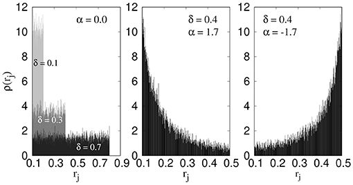
Figure 1. Distributions of link radii rj for different values of the power α and width δ. For α = 0 all the radii within the interval have equal probability whereas for positive and negative values of α there is higher probability to have narrow and wide links, respectively.
4. Numerical Results From DPNM
We perform simulations with constant global pressure drop ΔP and evolve the systems to steady state, where the macroscopic quantities fluctuate around a steady average. In the steady state, we measure the total flow rate Q. Results are averaged over 20 different realizations of the pore network. By fitting the numerical data with Equation (3) for the low capillary number regime, we calculate the exponent β and the threshold pressure Pc. As there are two parameters to determine from each data set, we considered a method of minimizing the error related to the least square fit (Sinha and Hansen, 2012). We illustrate this procedure briefly here. First we choose a trial value of β and perform least square fitting with the data points. This will provide a value of Pc and an error associated with it. We perform this for a set of β values and find the corresponding error values. We then plot the errors as a function of β. This is shown in Figure 2 for five different saturations where we see non-monotonic behavior of the errors with a minimum. We then consider the value of β that corresponds to the minimum error and use the corresponding value of Pc. When plotting log(ΔP − Pc) with logQ, we find the crossover point between a non-linear and a linear regime from eye approximation. From this crossover, we then identify the crossover pressure drop Pt.
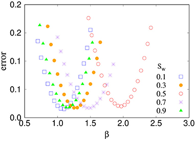
Figure 2. The error associated with least-square fitting of the numerical results to Equation (3) as a function of the trial values of β. Results are shown for five different saturations Sw. The minima of these plots decide the final values of β and Pc.
In the following we present the results showing how the steady-state rheology depends on the three parameters, (A) the wetting saturation Sw, (B) the power α, and (C) the width δ related to the pore-size distribution. Sw is varied between 0 and 1. We keep rmin = 0.1 and vary rmax from 0.2 to 0.8. In case of real a porous media, the pore sizes generally vary over a few orders of magnitude. In the pore-network simulations however, making the pores very small will lead the simulations to reach the steady state in a slower rate and will make the simulations computationally very expensive. Furthermore, as we will see in the following, δ do not affect the value of the exponent β and only controls the crossover point. We therefore considered δ to vary from 0.1 to 0.7 in the present study. The exponent α is varied in the range −2.0 ≤ α ≤ 2.0. We will focus on the non-linear exponent β and the pressure Pt related to the cross-over from non-linear to linear regime. Then in a Pt vs. β plane we will highlight how the two quantities vary when we change the values of Sw, α and δ.
4.1. Effect of Sw
The variation of the flow rate Q with the pressure drop ΔP is shown in Figure 3 for three different wetting saturations (Figure 3A) 0.1, (Figure 3B) 0.5, and (Figure 3C) 0.9 where we plotted log(Q) as a function of log(ΔP − Pc). The value of α and δ are kept constant here at 0.0 and 0.3, respectively. The respective threshold pressures (Pc), measured by the minimum error method, are indicated in the plots. All the plots show a non-linear regime at lower pressure drops and then a crossover to a linear regime. However, the slope in the non-linear regime is much higher for Sw = 0.5 than 0.1 or 0.9. Similarly, the threshold pressure Pc is also higher for Sw = 0.5. This indicates the fact that as Sw → 0 or Sw → 1, the two-phase flow essentially approach to the single phase flow and it should eventually follow the linear Darcy law without any threshold pressure. In order to see the nature of this variation toward the linear regime, we plot in Figures 3D–F, the values of β and Pt and Pc as a function of Sw, where Sw is varied from 0.1 to 0.9 with an interval of 0.1. All three plots show a peak around Sw = 0.5 with β = 1.97 and then continuously decrease in both sides. The decrease in both β and Pt suggests that not only the non-linearity gradually disappears as Sw deviates from 0.5, but also the linear Darcy regime can be obtained at a relatively lower pressure drop. At the same time, the overall threshold pressure Pc also decreases as the saturation approaches to 0 or 1.
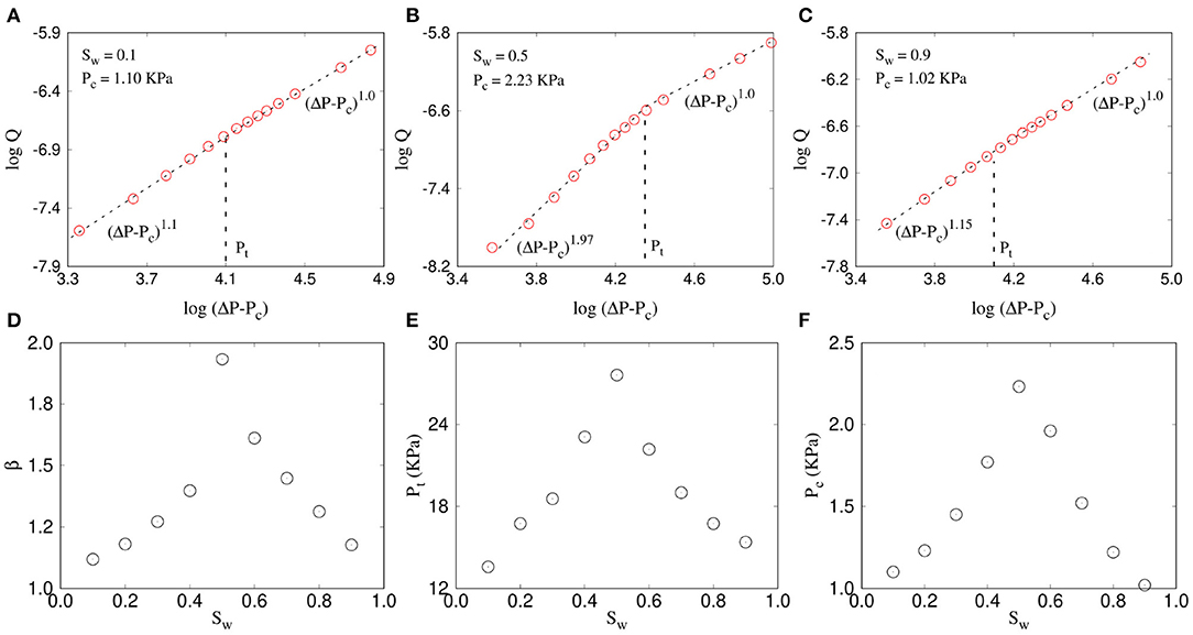
Figure 3. Plot of ΔP − Pc (Pa) vs. Q (m3/s) for a network of 64 × 64 links in 2D for three different wetting saturations Sw = 0.1, 0.5, and 0.9 are shown in (A–C), respectively. The plots show a non-linear regime at low pressure drop and a liner regime at high pressure drop. The variations of the slopes β in the non-linear regime, the crossover pressure drop Pt (KPa) and the threshold pressure Pc (KPa) as a function of Sw are shown in (D–F), respectively. All the β, Pt, and Pc have a maximum around Sw = 0.5 and decreases on either side.
If we consider that the flow occurs in channels with capillary barriers (Roux and Herrmann, 1987), that is, the increase in Q with ΔP is contributed from two factors, the increase in the number of conducting flow paths and the increase in the flow in each path, then that explains the reduction in both β and Pt as Sw → 0 or 1. As the saturation of a certain fluid decreases, either it reduces the number of fluid-fluid interfaces or produces smaller bubbles of one fluid. In both the cases the effective capillary barriers corresponding to any flow path decreases. This results in more flow paths with one fluid or with negligible capillary barriers which will start flowing as soon as any pressure drop is applied, making the β to move toward 1. At the same time, the maximum capillary barrier that the model needs to overcome to make all possible paths flowing also decreases, which moves the non-linear to linear transition point to a lower value of ΔP. Experimental observation of the variation of β with saturation was first reported in Rassi et al. (2011). No threshold pressure was considered in that study while analyzing the results. A recent experimental study (Zhang et al., 2021) explores the variation of β and the crossover point as a function of fractional flow, Fw = Qw/Q. By balancing the surface energy to create fluid meniscus to the injection energy, they developed a theory that can predict the crossover point between the two regimes they have studied. However, they have studied the crossover from the linear regime at very low pressure drop to the non-linear regime at the intermediate pressure drop, whereas our present study addresses the crossover from the non-linear regime at the intermediate pressure drop to the linear regime at high pressure drop.
4.2. Effect of α
The power α related to the pore-size distribution function defined in Equation (28) determines the shape of the distribution and tells us how the probability of having the wider pores are compared to the narrower ones. All the pore radii within the range δ are equally probable for α = 0 whereas positive and negative values of α indicate lower or higher probability of having wider pores, respectively (Figure 1). As the interfacial pressures are inversely proportional to ri (Equation 27), the local capillary barriers are larger for α > 0 compared to α < 0. In Figure 4, we plot log(ΔP − Pc) with log(Q) for three different values of α (Figure 4A) 0, (Figure 4B) 0.5, and (Figure 4C) −0.5. The wetting saturation and the distribution width are kept constant here at Sw = 0.5 and δ = 0.3, respectively. A few things are to be noticed. The non-linear regime here is highly influenced by the value of α whereas the slope in linear regime remains at ≈ 1 independent of α. The exponent β is maximum for α = 0, and then falls to 1.46 and 1.58 at α = 0.5 and −0.5, respectively. Moreover, the threshold pressure Pc also decreases with the increase of |α|. The decrease in Pc for α < 0 is intuitive, since the wider pores are in larger quantity compared to smaller pores, which will cause a less capillary barrier to start the flow. The decrease in Pc for α > 0 is rather counter intuitive and may be related to the decrease in slope in the non-linear regime.
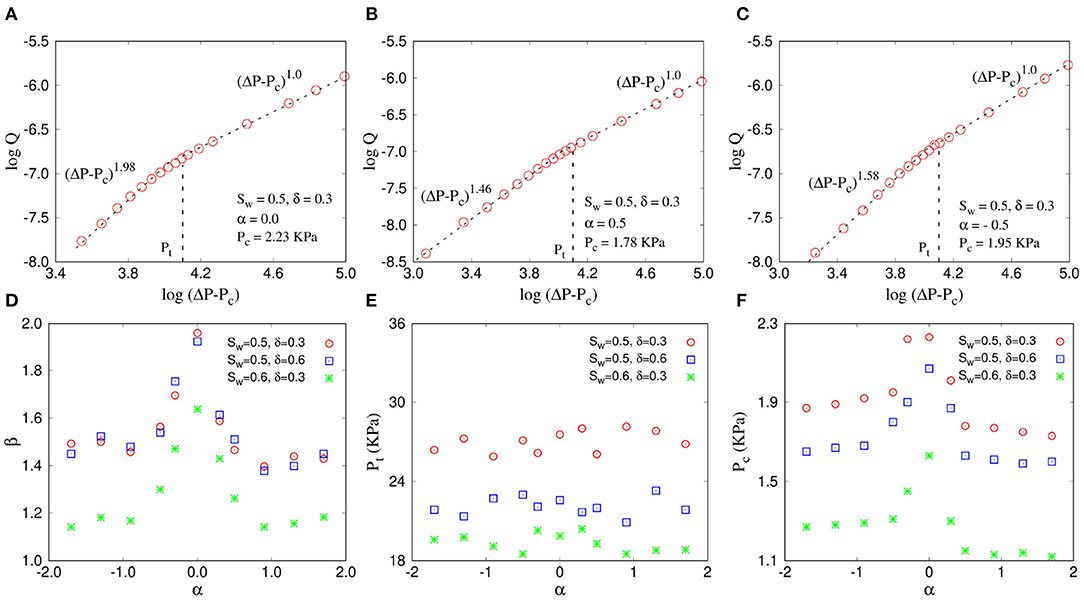
Figure 4. Variation of Q (m3/s) as a function of ΔP − Pc (Pa) for a network of 64 × 64 links and for α = 0, +0.5, and −0.5 are shown in (A–C), respectively. The wetting saturation Sw = 0.5 and the distribution width δ = 0.3 here. The variations of the slopes β in the non-linear regime, the crossover pressure drop Pt (KPa) and the threshold pressure Pc (KPa) as a function of Sw are shown in (D–F), respectively where β has a maximum at α = 0 whereas Pt does not show any specific dependence on α. Pc has a maximum around α = 0 and decreases on either side.
In Figure 4D, we plot β as a function of α which shows the decreasing trends of β on both sides of α = 0 and then becomes constant after it reaches to ≈ 1.5 around |α| = 1. This indicates that any change in the fluctuations among the link radii than the uniform distribution causes slower increase in the conductive paths when increasing the ΔP. The crossover pressure drop Pt is plotted in Figure 4E which shows that Pt remains constant independent of the value or sign of α. Figure 4F shows that Pc shows a maximum at Sw = 0.5 and decreases on either side. The decrease of Pc for negative α is understandable as there will more links with larger radius in this case. For positive α we have less links with large radius. Pc is still observed to decrease, most probably because of the nature of the fitting since β decreases here.
Notice that, such a variation in the non-linear exponent β while varying α was not observed in case of CFBM where β has a value of 3/2 irrespective of the radii distribution (Equation 25). This indicates that the mixing of the fluids at the nodes in a pore network has more complex effect than the flow in individual channels in CFBM. The crossover point Pt here is analogous to the maximum threshold PM in CFBM which do not depend on α in both the models as it only depends on the span of the distribution and not on the shape. Therefore, as we will see in the next section, Pt has a strong dependence on δ, the span of the distribution.
4.3. Effect of δ
We now perform simulations by varying the width of the radii distribution give by, δ = rmax − rmin = 0.1, 0.2, 0.3, 0.5, and 0.7, where rmin was kept constant at 0.1. The wetting saturation and the distribution power are kept constant here at Sw = 0.5 and α = 0, respectively. The results are illustrated in Figure 5. Interestingly, unlike the variation of β with the distribution power α as seen before, here the slopes in the non-linear regime are almost independent of the distribution width δ and remains constant around 2.0 (Figure 5A). The crossover pressure drop Pt, on the other hand, decreases with increase in δ, which was almost constant when we varied the distribution power α. We also found that the global threshold pressure Pc gradually decreases with increasing δ, from Pc ≈ 2.5KPa at δ = 0.1 to ≈ 1.5KPa at δ = 0.7. This is because as we increase δ, rmax also increases and the system contains more pores with larger pore radii. This decreases the capillary barriers and hence reduces the global threshold pressure Pc.
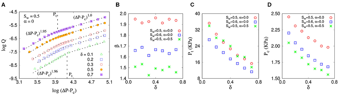
Figure 5. (A) Plot of Q (m3/s) vs. ΔP − Pc (Pa) when varying the distribution width δ where the slopes in the non-linear, as well as in the linear regimes do not show any variation with δ. In (B–D), respectively, we show the variation of β, Pt (KPa) and Pc (KPa) with δ.
4.4. The Pt vs. β Plane
To illustrate the all variations in the rheological behavior as a function of different parameters, we constructed a Pt − β plane. This is shown in Figure 6. We indicate all the data points there corresponding to the three sets. The variation in the β and Pt as we increase Sw, α, and δ are indicated by arrows in the plot. They can be summarized as:
Varying α: When α is increased, β decreases keeping Pt constant, and the points moves to left along a horizontal line (green squares).
Varying δ: When δ is increased, Pt decreases keeping β constant, and the points move down along a vertical line (red circles).
Varying Sw: When Sw deviates from 0.5, both β and Pt decreases and the points move to lower values along a diagonal line (purple triangles).
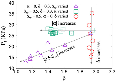
Figure 6. The Pt − β plane, which shows the effect of varying Sw, α, and δ on the rheological behavior. As Sw deviates from 0.5 (triangles), both β and Pt decreases. On the other hand, with increasing α (squares) and δ (circles), respectively, either β or Pt decreases keeping the other one constant.
5. Discussion
In this article we explored how the rheological properties two-phase flow in porous media in steady state is affected by the underlying system disorder. We performed analytical calculations with a capillary bundle model and numerical simulations with dynamic pore-network model. We varied the shape and width of the distribution of the pore-radii with two distribution parameters α and δ, respectively, and studied the transition from a non-linear flow regime to a linear Darcy flow. We found that the exponent β related to the non-linearity is equal to 3/2 for the capillary bundle model and do not depend on α. For the pore-network model on the other hand, β ≈ 2 for uniform distribution (α = 0) and approaches toward 1.5 as |α| is increased. The width δ of the distribution affects the crossover point Pt in both the models. When δ is increased, the linear regime becomes achievable at a relatively lower pressure drop. Both β and Pt depends on the saturation Sw. As Sw deviates from 0.5, the two-phase flow moves closer to single phase flow and both β and Pt decreases simultaneously making the linear region more and more prominent. These numerical results can be explained qualitatively with the hypothesis that the total flow rate is contributed from the number of conducting paths and the flow in those paths (Roux and Herrmann, 1987), which makes it to increase faster than a linear behavior.
It is worth mentioning here that the single phase flow of Bingham fluid in porous media also shows similar non-linearity with a global yield threshold and a crossover to a linear regime (Roux and Herrmann, 1987; Talon and Bauer, 2013; Chevalier and Talon, 2015). Nash and Rees (2017) has studied Bingham fluid flow in one dimension and obtained different relations between applied pressure drop and Darcy velocity depending on the distribution of channel widths. Talon et al. (2014) have analytically explored the flow of Bingham fluid in 1d channels with aperture variation and observed different scaling between pressure drop and flow rate depending on such variation in apertures. Above studies support the fact that, when up-scaled to a certain pore-network, both Bingham flow and two-phase flow is affected by the pore-size distribution and hence the topology of the network.
The dependency of the effective rheological properties on the pore-size distribution indicates a possibility to predict the transport properties directly from the geometrical properties of the porous media. Puyguiraud et al. (2021) in a recent letter developed a model for single phase flow for the prediction of transport from knowledge of the characteristic pore length and of the Eulerian velocity distribution. Another approach is based on the Hadwiger theorem stating that any extensive function (such as the free energy) describing the flow may be expressed in terms of the Minkowski functionals describing the geometry of the porous medium. The transport properties may then be found from the free energy (see Khanamiri et al., 2018). Roy et al. (2020) proposed a framework that connects the average seepage velocities to the distribution of local fluid velocities. This means, obtaining the velocity or flow distribution from the distribution of pores is the missing link that would allow the prediction of hydrodynamic transport from geometrical information only. For random bead packs, Coppersmith et al. (1996) showed that the variations of contact angles allow for the relation between distribution of throat radii and the distribution of the flow fractions that depart a pore body. With that, Alim et al. (2017) proposed an approach for single phase flow to predict the flow distribution from the geometrical properties of porous media that is based on Kirchhoff's law for fluid mass conservation coupled with assumptions on the distribution of coordination numbers of pore bodies. There are more studies on the local velocity distribution for single phase flow (Siena et al., 2014; Wu et al., 2016; De Anna et al., 2017; Aramideh et al., 2018; An et al., 2020; Souzy et al., 2020), but detailed study for two-phase flow are lacking. Furthermore, Alim et al. (2017) also emphasized that, in addition to the distribution of pore sizes, the local correlations between adjacent pores are necessary to predict the flow distribution. The observation in our present study, that the non-linear exponent β does not depend on the radii distribution in case of the capillary bundle with disconnected links, whereas it varies continuously with the distribution for the pore-network, also indicates the same, that the network connectivity plays a key role in the transport properties in addition to the pore-size distribution. In our present study we considered a fixed coordination number, and therefore further study is necessary to explore the role of network connectivity on the effective rheology.
Data Availability Statement
The raw data supporting the conclusions of this article will be made available by the authors, without undue reservation.
Author Contributions
SR and AH performed all the analytical derivations related to CFBM. The code for DNPM was written by SS. SR performed all numerical simulations and data analysis related to DNPM. The initial draft of the manuscript was written by SR and SS which was then updated by all the authors. All authors contributed to the article and approved the submitted version.
Funding
This work was partly supported by the Research Council of Norway through its Centers of Excellence funding scheme, project number 262644. SS was partially supported by the National Natural Science Foundation of China under grant number 11750110430.
Conflict of Interest
The authors declare that the research was conducted in the absence of any commercial or financial relationships that could be construed as a potential conflict of interest.
Publisher's Note
All claims expressed in this article are solely those of the authors and do not necessarily represent those of their affiliated organizations, or those of the publisher, the editors and the reviewers. Any product that may be evaluated in this article, or claim that may be made by its manufacturer, is not guaranteed or endorsed by the publisher.
Footnotes
1. ^The values in the brackets are the exponents reported in the literature, the reciprocals of them should be compared here, as we express our results as Q as a power law in ΔP, whereas the cited articles expressed ΔP as a power law in Q, or rather the corresponding capillary number Ca.
References
Aker, E., Maloy, K. J., Hansen, A., and Batrouni, G. G. (1998). A two-dimensional network simulator for two-phase flow in porous media. Transp. Porous Med. 32:163. doi: 10.1023/A:1006510106194
Alim, K., Parsa, S., Weitz, D. A., and Brenner, M. P. (2017). Local pore size correlations determine flow distributions in porous media. Phys. Rev. Lett. 119:144501. doi: 10.1103/physrevlett.119.144501
An, S., Hasan, S., Erfani, H., Babaei, M., and Niasar, V. (2020). Unravelling effects of the pore-size correlation length on the two-phase flow and solute transport properties: GPU-based pore-network modeling. Water Resour. Res. 56:e2020WR027403. doi: 10.1029/2020WR027403
Aramideh, S., Vlachos, P. P., and Ardekani, A. M. (2018). Pore-scale statistics of flow and transport through porous media. Phys. Rev. E 98:013104. doi: 10.1103/PhysRevE.98.013104
Batrouni, G. G., and Hansen, A. (1988). Fourier acceleration of iterative processes in disordered systems. J. Stat. Phys. 52:747. doi: 10.1007/BF01019728
Chen, J. D., and Wilkinson, D. (1985). Pore-scale viscous fingering in porous media. Phys. Rev. Lett. 55:1892. doi: 10.1103/PhysRevLett.55.1892
Chevalier, T., Salin, D., Talon, L., and Yiotis, A. G. (2015). History effects on nonwetting fluid residuals during desaturation flow through disorderedporous media. Phys. Rev. E 91:043015. doi: 10.1103/PhysRevE.91.043015
Chevalier, T., and Talon, L. (2015). Generalization of Darcys law for Bingham fluids in porous media: from flow-field statistics to the flow-rate regimes. Phys. Rev. E 91:023011. doi: 10.1103/PhysRevE.91.023011
Coppersmith, S. N., Liu, C. -H., Majumdar, S., Narayan, O., and Witten, T. A. (1996). Model for force fluctuations in bead packs. Phys. Rev. E 53:4673. doi: 10.1103/physreve.53.4673
De Anna, P., Quaife, B., Biros, G., and Juanes, R. (2017). Prediction of the low-velocity distribution from the pore structure in simple porous media. Phys. Rev. Fluids 2:124103. doi: 10.1103/PhysRevFluids.2.124103
Dullien, F. A. L. (1992). Porous media: Fluid, transport and pore structure. San Diego, CA: Academic Press.
Gao, Y., Lin, Q., Bijeljic, B., and Blunt, M. J. (2020). Pore-scale dynamics and the multiphase Darcy law. Phys. Rev. Fluids 5:013801. doi: 10.1103/PhysRevFluids.5.013801
Gunstensen, A. K., Rothman, D. H, Zaleski, S, and Zanetti, G. (1991). Lattice Boltzmann model of immiscible fluids. Phys. Rev. A 43:4320. doi: 10.1103/PhysRevA.43.4320
Hansen, A., Hemmer, P. C., and Pradhan, S. (2015). The Fiber Bundle Model: Modeling Failure in Materials. Berlin: Wiley.
Joekar-Niasar, V., and Hassanizadeh, S. M. (2012). Analysis of fundamentals of two-phase flow in porous media using dynamic pore-network models: a review. Crit. Rev. Environ. Sci. Technol. 42:1895. doi: 10.1080/10643389.2011.574101
Khanamiri, H. H., Berg, C. F., Slotte, P. A., Schlüter, S., and Torsaeter, O. (2018). Description of free energy for immiscible two-fluid flow in porous media by integral geometry and thermodynamics. Water Resour. Res. 54, 9045–9059. doi: 10.1029/2018WR023619
Kirkpatrick, S. (1973). Percolation and conduction. Rev. Mod. Phys. 45:574. doi: 10.1103/RevModPhys.45.574
Lenormand, R., Touboul, E., and Zarcone, C. (1988). Numerical models and experiments on immiscible displacements in porous media. J. Fluid Mech. 189:165. doi: 10.1017/S0022112088000953
Lenormand, R., and Zarcone, C. (1985). Invasion percolation in an etched network: measurement of a fractal dimension. Phys. Rev. Lett. 54:2226. doi: 10.1103/PhysRevLett.54.2226
Måløy, K. J., Feder, J., and Jøssang, T. (1985). Viscous fingering fractals in porous media. Phys. Rev. Lett. 55:2688. doi: 10.1103/PhysRevLett.55.2688
Nash, S., and Rees, D. A. S. (2017). The effect of microstructure on models for the flow of a Bingham fluid in Porous media: one-dimensional flows. Transp. Porous Med. 116:1073. doi: 10.1007/s11242-016-0813-9
Puyguiraud, A., Gouze, P., and Dentz, M. (2021). Pore-scale mixing and the evolution of hydrodynamic dispersion in porous media. Phys. Rev. Lett. 126:164501. doi: 10.1103/PhysRevLett.126.164501
Rassi, E. M., Codd, S. L., and Seymour, J. D. (2011). Nuclear magnetic resonance characterization of the stationary dynamics of partially saturated media during steady-state infiltration flow. New J. Phys. 13:015007. doi: 10.1088/1367-2630/13/1/015007
Roux, S., and Herrmann, H. J. (1987). Disorder-induced nonlinear conductivity. Europhys. Lett. 4:1227. doi: 10.1209/0295-5075/4/11/003
Roy, R., Sinha, S., and Hansen, H. (2020). Flow-area relations in immiscible two-phase flow in porous media. Front. Phys. 8:4. doi: 10.3389/fphy.2020.00004
Roy, S., Hansen, A., and Sinha, S. (2019). Effective rheology of two-phase flow in a capillary fiber bundle model. Front. Phys. 7:92. doi: 10.3389/fphy.2019.00092
Scheidegger, A. E. (1974). The Physics of Flow Through Porous Media. Toronto, ON: University of Toronto Press.
Siena, M., Riva, M., Hyman, J. D., Winter, C. L., and Guadagnini, A. (2014). Relationship between pore size and velocity probability distributions in stochastically generated porous media. Phys. Rev. E 89:013018. doi: 10.1103/PhysRevE.89.013018
Sinha, S., Bender, A. T., Danczyk, M., Keepseagle, K., Prather, C. A., Bray, J. M., et al. (2017). Effective rheology of two-phase flow in three-dimensional porous media: experiment and simulation. Transp. Porous Med. 119:77. doi: 10.1007/s11242-017-0874-4
Sinha, S., Gjennestad, M. Aa., Vassvik, M., and Hansen, A. (2021). Fluid meniscus algorithms for dynamic pore-network modeling of immiscible two-phase flow in porous media. Front. Phys. 8:548497. doi: 10.3389/fphy.2020.548497
Sinha, S., and Hansen, A. (2012). Effective rheology of immiscible two-phase flow in porous media. Europhys. Lett. 99:44004. doi: 10.1209/0295-5075/99/44004
Sinha, S., Hansen, A., Bedeaux, D., and Kjelstrup, S. (2013). Effective rheology of bubbles moving in a capillary tube. Phys. Rev. E 87:025001. doi: 10.1103/PhysRevE.87.025001
Souzy, M., Lhuissier, H., Meheust, Y., Le Borgne, T., and Metzger, B. (2020). Velocity distributions, dispersion and stretching in three-dimensional porous media. J. Fluid Mech. 891:A16. doi: 10.1017/jfm.2020.113
Tallakstad, K. T., Knudsen, H. A., Ramstad, T., Løvoll, G., Måløy, K. J., Toussaint, R., et al. (2009a). Steady-state two-phase flow in porous media: statistics and transport properties. Phys. Rev. Lett. 102:074502. doi: 10.1103/PhysRevLett.102.074502
Tallakstad, K. T., Løvoll, G., Knudsen, H. A., Ramstad, T., Flekkøy, E. G., and Måløy, K. J. (2009b) Steady-state, simultaneous two-phase flow in porous media: an experimental study. Phys. Rev. E 80:036308. doi: 10.1103/PhysRevE.80.036308
Talon, L., Auradou, H., and Hansen, A. (2014). Effective rheology of Bingham fluids in a rough channel. Front. Phys. 2:24. doi: 10.3389/fphy.2014.00024
Talon, L., and Bauer, D. (2013). On the determination of a generalized Darcy equation for yield-stress fluid in porous media using a lattice-Boltzmann TRT scheme. Eur. Phys. J. E 36:139. doi: 10.1140/epje/i2013-13139-3
Valavanides, M. (2018). Review of steady-state two-phase flow in porous media: independent variables, universal energy efficiency map, critical flow conditions, effective characterization of flow and pore network. Transp. Porous Med. 123:45. doi: 10.1007/s11242-018-1026-1
Washburn, E. W. (1921). The dynamics of capillary flow. Phys. Rev. 17:273. doi: 10.1103/PhysRev.17.273
Whitaker, S. (1986). Flow in porous media I: a theoretical derivation of Darcy's law. Transp. Porous Med. 1:3. doi: 10.1007/BF01036523
Wilkinson, D., and Willemsen, J. F. (1983). Invasion percolation: a new form of percolation theory. J. Phys. A 16:3365. doi: 10.1088/0305-4470/16/14/028
Witten, T. A. Jr., and Sander, L. M. (1981). Diffusion-limited aggregation, a kinetic critical phenomenon, Phys. Rev. E 47:1400. doi: 10.1103/PhysRevLett.47.1400
Wu, A., Liu, C., Yin, S., Xue, Z., and Chen, X. (2016). Pore structure and liquid flow velocity distribution in water-saturated porous media probed by MRI. Trans. Nonferrous Met. Soc. China 26:1403. doi: 10.1016/S1003-6326(16)64208-5
Yiotis, A. G., Talon, L., and Salin, D. (2013). Blob population dynamics during immiscible two-phase flows in reconstructed porous media. Phys. Rev. E 87:033001. doi: 10.1103/PhysRevE.87.033001
Zhang, Y., Bijeljic, B., Gao, Y., Lin, Q., and Blunt, M. J. (2021). Quantification of non-linear multiphase flow in porous media. Geophys. Res. Lett. 48:e2020GL090477. doi: 10.1029/2020GL090477
Keywords: non-linear fluid flow, two-phase flow, porous media, pore-size distribution, effective rheology
Citation: Roy S, Sinha S and Hansen A (2021) Role of Pore-Size Distribution on Effective Rheology of Two-Phase Flow in Porous Media. Front. Water 3:709833. doi: 10.3389/frwa.2021.709833
Received: 14 May 2021; Accepted: 02 July 2021;
Published: 30 July 2021.
Edited by:
Charlotte Garing, University of Georgia, United StatesReviewed by:
Alexandre Puyguiraud, Instituto de Diagnóstico Ambiental y Estudios del Agua (IDAEA), SpainJesse Dickinson, United States Geological Survey (USGS), United States
Copyright © 2021 Roy, Sinha and Hansen. This is an open-access article distributed under the terms of the Creative Commons Attribution License (CC BY). The use, distribution or reproduction in other forums is permitted, provided the original author(s) and the copyright owner(s) are credited and that the original publication in this journal is cited, in accordance with accepted academic practice. No use, distribution or reproduction is permitted which does not comply with these terms.
*Correspondence: Subhadeep Roy, subhadeeproy03@gmail.com