Water Quality Sampling Frequency Analysis of Surface Freshwater: A Case Study on Bristol Floating Harbour

Introduction

The ability to monitor water quality is critical to managing precious freshwater resources for drinking water, recreation and ecosystem support purpose. As climate-related and other anthropogenic impacts on water quality increase, it is more and more important to be able to design monitoring networks that provide real time information on water quality, and track short, medium and long term changes in water quality.

Designers of water quality networks (WQMNs) must consider a range of factors including monitoring locations, water quality parameters, frequency of sampling, identify human and technical resources, as well as constraints such as cost, accessibility, data collection and handling in order to design a program that meets the overall purpose of the monitoring network (Behmel et al., 2016). Until the 21st century, water quality monitoring networks (WQMNs) were typically reliant on manual (grab) sampling, followed by transportation to a laboratory for chemical and biological analysis (Strobl and Robillard, 2008; Tapparello et al., 2017). This provides adequate information for long-term monitoring of many water quality parameters but it can become time consuming and costly if needs to provide data for analysing short-term trends or changes in time and indeed may be impractical for detecting rapid changes in variables that are highly sensitive to weather and other environmental influences, for example turbidity, temperature, conductivity and dissolved oxygen and dissolved organic matter (Ivanovsky et al., 2016). These manual networks are highly dependent on human interaction time to obtain results due to transportation of samples and potential loss of quality control (Tapparello et al., 2017), and sometimes during extreme events involve health and safety risks.

Two key technological advances have significantly changed collection of water quality data and can overcome disadvantages of manual sampling. The first of these is the use of in-situ sensors to provide high frequency measurement of a range of physical and chemical water quality parameters without the need for labour-intensive grab sampling and laboratory analysis. The second is the ability to connect these in-situ sensors to wireless sensor networks, significantly increasing both the amount of data that can be collected and the ability to observe water quality in real time (Kirchner et al., 2004; Halliday et al., 2015; Chen and Han, 2018).

This type of high frequency data supports a range of applications including water quality forecasting models, compliance monitoring, baseline characterisation and event based monitoring. However, a very high volume of data is not necessarily an advantage as consideration also needs to be given to capacity to store, handle and process data as well as associated costs. There is a need to optimise the frequency vs. manageability of data, however this optimisation will vary depending on the overall purpose of any monitoring network. Further, these networks need to be set up in advance, and have limited flexibility in terms of responding to unexpected events at different locations.

Naddeo et al. (2007) and Liu et al. (2013) used statistical techniques to optimise low frequency (monthly or daily) datasets, and only two studies have been identified that deal with high frequency datasets (Anvari et al., 2009; Zhou et al., 2018).

This study further explores the issue of frequency optimisation by applying three different statistical approaches for determining the optimum sampling frequency for different water quality parameters using a high frequency dataset. It intends to determine the minimum frequency required to communicate periodic fluctuations in water quality and investigate the additional benefit of recording data at a frequency higher than the minimum required.

Three approaches are tested: (i) Analysing the frequency components of each parameter at each site to quantify the Nyquist frequency and supposed minimum sampling rate for determination of periodic fluctuations, proposed by Zhou (1996) and Khalil and Ouarda (2009). (ii) Using spectral analysis to determine the Power Spectral Density cumulation curve (Otis and Solomon, 1991) to determine reasonable frequencies to monitor water quality determinants; for each frequency evaluate the loss of information (da Silva et al., 2019). (iii) Analysing the limits of the spectral analysis computing spectrograms using Wavelet analysis (Torrence and Compo, 1998).

The proposed approaches are tested utilising a high frequency dataset built from recording continuous physical and chemical water quality parameters (conductivity, dissolved organic matter, dissolved oxygen, temperature, turbidity) with multiparameter sondes at 3 sites in Bristol's Floating Harbour. This dataset has been obtained by building on the work of Chen and Han (2018).

In this paper, a background section (section Background) is presented which reviews the use of wireless sensors in water quality monitoring networks, the benefits of high frequency monitoring. The importance of selecting a suitable sampling frequency is also discussed. In section Materials and Methods, relevant information about the history and known dynamics of the Floating Harbour are presented and the methods of data collection and frequency analysis are discussed. Results are presented in section Results, followed by the discussion (section Discussion and Conclusions) about the suitability and limitations of the different approaches used to assess and select sampling frequencies and possible areas for further research.

Background

Use of Wireless Sensor Networks for Water Quality Monitoring

In recent decades, wireless sensor networks (WSNs) have been developed and are being increasingly deployed by researchers, councils and commercial companies alike for water quality monitoring. General WSN system architecture consists of data acquisition, transmission, processing, storage and redistribution (Tapparello et al., 2017; Chen and Han, 2018; Hadimani et al., 2021). Data acquisition is achieved by a network of in-situ sensor(s) using a given sampling frequency, and these sensor probes have evolved to now be capable of measurement a broad range of physicochemical parameters such as conductivity, turbidity, dissolved oxygen (DO) and pH (Marcé et al., 2016). Collected data is transferred to the central monitoring hub by technologies commonly including cellular networks such as GSM or newer networks including ZigBee or even Wi-Fi. These networks are expected to continue to develop as the Internet of Things (IoT) grows commercially and gains research attention. Once transferred, the data can be processed, stored, and analysed. Technologies such as these make possible remote continuous real-time monitoring and visualisation of water-body quality parameters at fixed locations (Tapparello et al., 2017; Chen and Han, 2018; Hadimani et al., 2021) and have been found to better describe water-bodies when compared to manual methods, allowing the understanding of biogeochemical processes (Kirchner et al., 2004; Ivanovsky et al., 2016).

WSNs offer much freedom in the selection of frequency for monitoring water quality parameters, with systems monitoring at low frequency being prone to uncertainty (Birgand et al., 2013). A review by Khalil and Ouarda (2009) found that the use of multiparameter sondes and the much finer possible temporal sampling resolutions were able to capture transient events likely to have been missed by grab sampling; this is particularly important for flashy streams where timing sampling with peak flow is challenging. However, despite high-frequency data collection not incurring excessive cost, there are constraints to data transfer and storage in systems without automated telemetry (Chappell et al., 2017). Also, too high a monitoring frequency can return redundant information (Khalil and Ouarda, 2009), increasing potential noise in the data, as well as power demand, increasing capital cost of setting up a renewable source (e.g., a solar panel) if mains electricity is unavailable. These considerations necessitate finding a balance in frequency for analysis of each physicochemical parameter.

Frequency Considerations in Water Quality Monitoring Network Design

There is no universally accepted method of designing a WQMN (Strobl and Robillard, 2008), yet it is a general consensus that a successful design is dependent on the clear definition of system objectives, which should identify the information to be gathered (Bartram and Ballance, 1996; Khalil and Ouarda, 2009; Behmel et al., 2016). The monitoring objectives are often set to provide the information necessary for water quality management, for example to meet legislative targets, mitigate immediate threats to human health, or improve long-term biodiversity and eco-system quality (Bartram and Ballance, 1996). As summarised by Strobl and Robillard (2008), monitoring programs must be designed with consideration given to the type of water body and classification system, capabilities of the existing network and pressures and risks associated with that water body. A monitoring network can then be designed by selecting (i) The variables to be monitored, (ii) the spatial arrangement and density of sampling sites, and (iii) the frequency of measurements to fulfil monitoring objectives (Bartram and Ballance, 1996; Strobl and Robillard, 2008).

Jiang et al. (2020) highlighted how the quantitative design of an optimal WQMN is very challenging. Defining the sampling frequency when designing a water quality monitoring network has a key role in determining the efficiency of the network, affecting both data quality and operation costs.

When defining the sampling frequency a range of consideration should be addressed (Table 1).

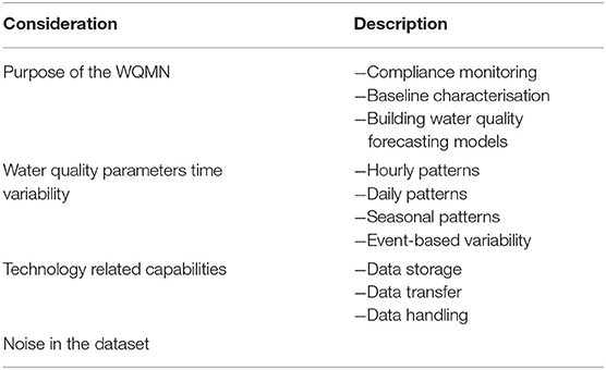
Table 1. Considerations to address when defining the sampling frequency for a high frequency WQMN.

The selection of the sampling frequency is influenced by the purpose of the WQMN. The need for different level of accuracy in representing the water quality changes according to the purpose of the WQMN: a network designed for routine water quality cheques will not need the same accuracy of a network that is created for water quality forecast or for identification of sources of pollution.

The sampling frequency changes with the type of parameters that are selected to be monitored in the WQMN. Different water quality parameters are affected by different external factors (i.e., tide, rainfall, solar radiation), hence defining a unique sampling frequency for the whole monitoring network is not ideal.

By sampling too frequently the obtained information is redundant and expensive furthermore will contain noise, while if the frequency is too low the collected data will represent an inaccurate water quality pattern (Skeffington et al., 2015).

Approaches to Selection of Sampling Frequency

There are two main approaches when designing monitoring frequency for a water quality monitoring network: the low frequency and the high frequency approach. The low frequency approach can be useful when the intended outcome of the monitoring network is to characterise water quality over a long period to detect seasonal variation or long-term trends. In these cases, the recommended sampling frequencies range from monthly to tri-monthly or even half-yearly (Zhou, 1996; Naddeo et al., 2007; Guigues et al., 2013; Liu et al., 2013; Khalil et al., 2014). In small study areas or small rivers, a low frequency approach is not a suitable approach since discharges and atmospheric events cause more sudden changes in water quality. In literature, continuous high frequency monitoring strategies are suggested for small study areas, without providing statistical explanation to the chosen monitoring frequency (Anvari et al., 2009; Chen and Han, 2018).

According to Nguyen et al. (2019) qualitative criteria were used in literature to identify the monitoring frequencies based on the knowledge or requirements of stakeholders or adapted from existing regulations as well as quantitative methods such as confidence interval (CI), entropy, analysis of variance (ANOVA), and hierarchical cluster analysis (HCA).

Table 2 summarises the optimisation approaches used in both low and high frequency monitoring studies and the conclusions drawn in each study in relation to actual vs. optimum data frequency.

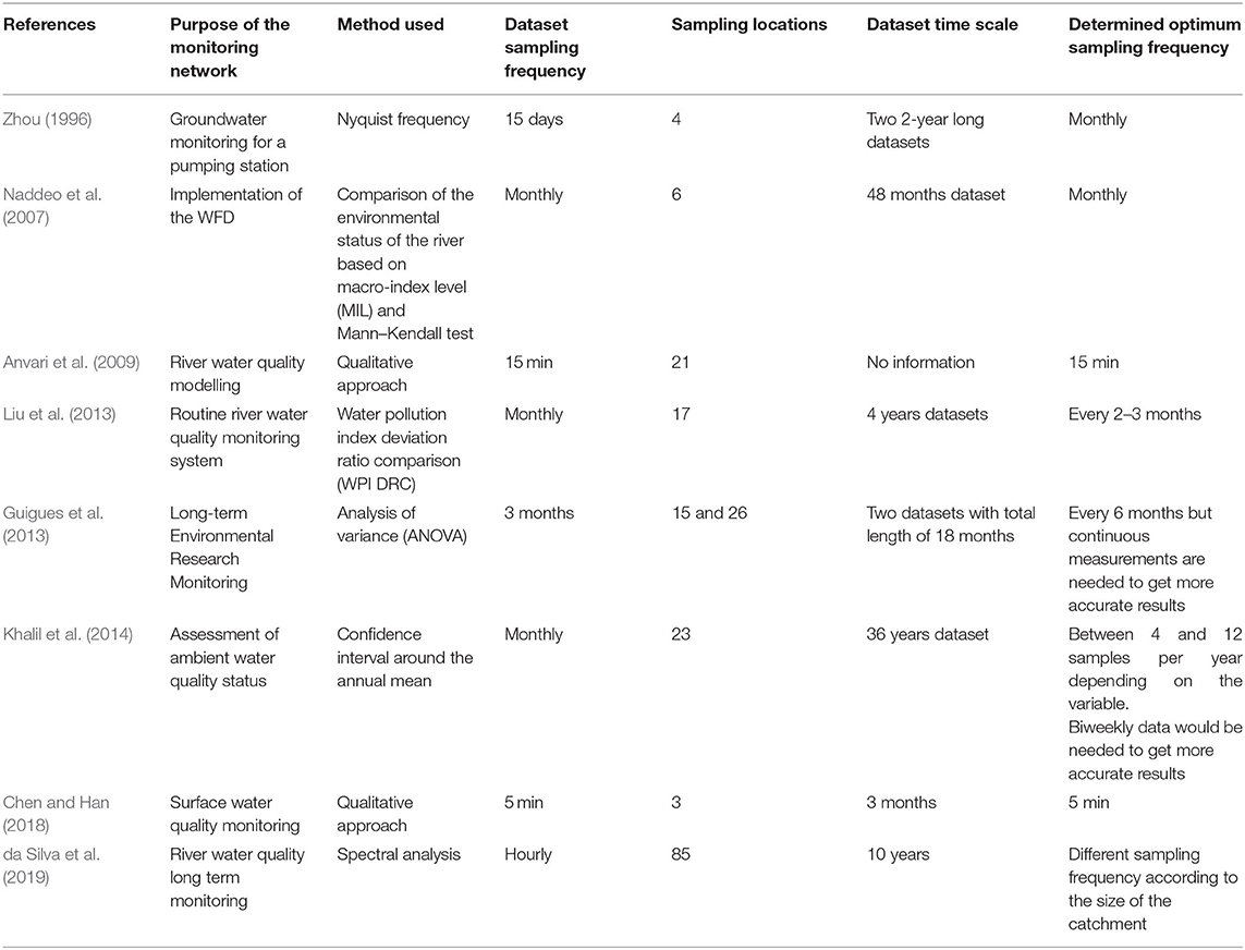
Table 2. Sampling frequency optimisation approaches used in literature.

In this paper three statistical approaches have been used to define a procedure to establish the appropriate sampling frequency for water quality parameters to be used when designing a high frequency monitoring quality network.

The first approach aims at finding the minimum sampling frequency for each water quality parameter to quantify the Nyquist frequency and supposed minimum sampling rate for determination of periodic fluctuations, proposed by Zhou (1996) and Khalil and Ouarda (2009).

The second approach proposed by da Silva et al. (2019) is used to determine reasonable frequencies to monitor water quality determinants and for each frequency evaluate the loss of information using the spectral analysis. It also used to determine the optimum sampling frequency in cases where there is no constant periodicity in the water quality parameter time series.

Lastly, to overcome the limits of the spectral analysis, a spectrogram is computed using Wavelet analysis (Torrence and Compo, 1998). This third approach completes the spectral analysis by adding information both the time and the frequency domain. The detailed methods for these are described in the next section.

Materials and Methods

Study Area

The historic Floating Harbour is at the heart of Bristol's city centre (Figure 1). Constructed in the 19th Century to rival Liverpool's shipping capabilities, the harbour is a large standing body of water retained by systems of locks. The harbour has evolved to be the setting for many recreational activities, notably paddle boarding and river cruises, while swimming in the harbour is not advised due to poor water quality. The old warehouses and shipping infrastructure have been transformed, regenerating the area as a tourist attraction and recreational area with museums, restaurants, and bars. Furthermore, the annual harbour festival each July brings influxes of visitors and residents to the harbour for demonstrations on the water, traditional sailing vessels, and street performances. The water quality in the harbour is therefore of value not just to the health of the ecosystem, but also to the city's heritage, tourism businesses and the value of adjacent properties.

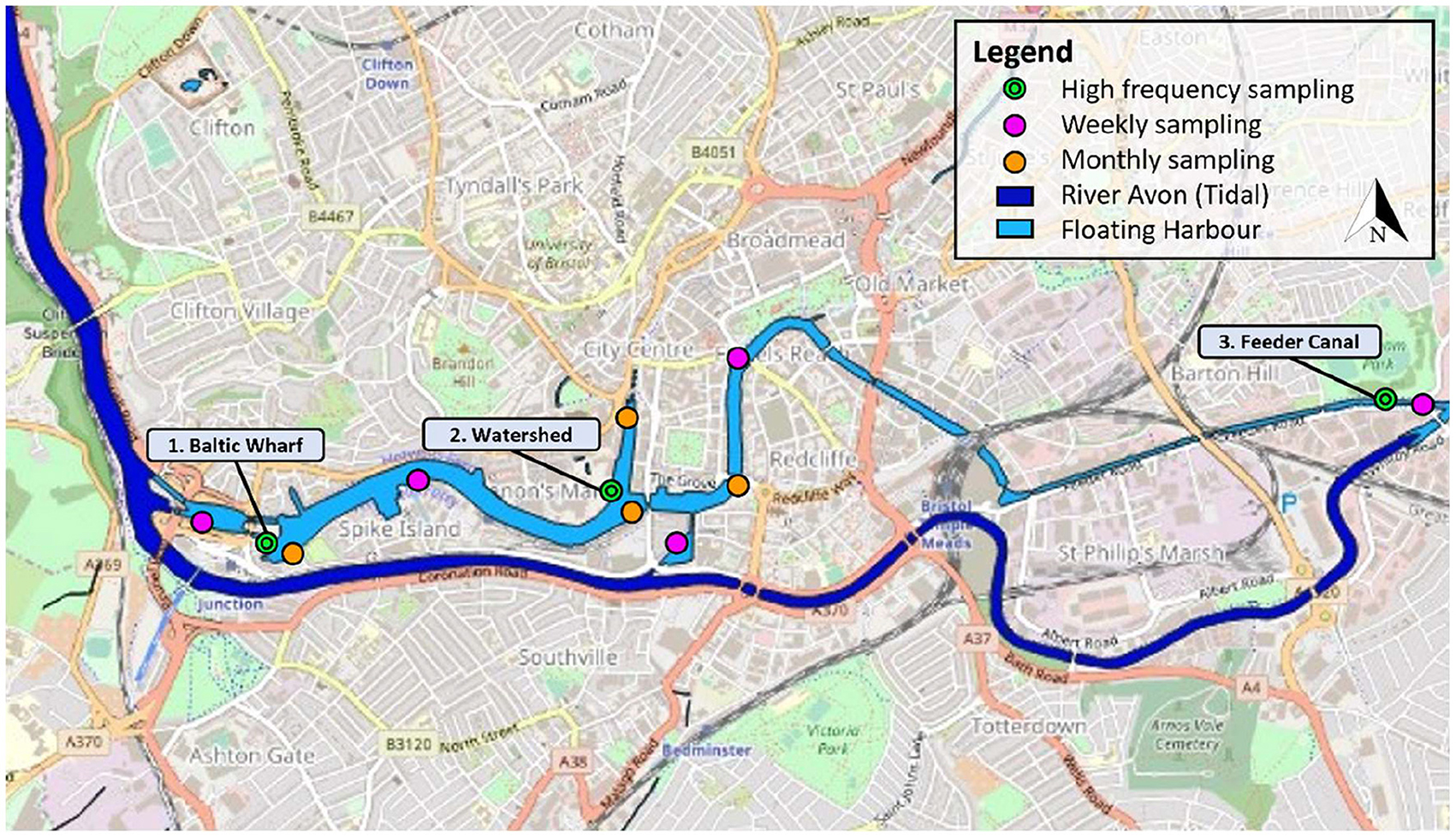
Figure 1. Bristol City Council sampling sites (Bristol City Council, 2019; Ordnance Survey, 2019) and monitoring stations used in this study.

It is primarily fed by the River Avon, which has most input into background water quality in the harbour. The Avon's catchment drains a large portion of the south west of England, taking in tributaries from the Cotswolds, Salisbury Plain and The Mendips before reaching Bristol, therefore having a number of potential polluting sources upstream including the sewage treatment works at Saltford and Keynsham and catchment runoffs (Bristol City Council, 2006). The Avon is tidal, hence the harbour experiences some limited saline intrusion through lock operations and spring tide, from the upstream and downstream locks. Henceforth in this study the harbour is compared to transitional waters or river systems where appropriate.

Also, at times of high flow and high tide, Mylne's culvert which transports the Bristol Frome beneath the harbour to the Avon new cut can become tidally locked, causing discharge into the harbour. This is the primary source of contamination at times of heavy rainfall. Other inputs include surface water and highway drains, which can negatively impact water quality, particularly during heavy rain after a dry spell. Much of the drainage in Bristol remains combined, hence there are three combined sewage overflows in the area, which according to Bristol City Council (2013) discharge infrequently. There are also moored boats at several locations—owners are required to follow proper waste discharge protocol, yet it is possible illegal disposal of sewage and grey water is taking place. Other minimal sources of pollution may include urile contamination from sewer rats or faecal contamination from water-bird populations. Lastly, the harbour is periodically scoured via the opening of locks at both ends of the harbour to prevent silt build-up at the Cumberland Basin. The scouring operations cause a drop in the water level in the harbour and resuspension of settled solids.

Historical Manual Sampled Datasets

Water quality in the Floating Harbour is currently monitored by grab sampling managed by Bristol City Council, with records of total coliforms, E-coli and Faecal streptococci beginning April 1994. The breadth of data has increased since then, with temperature, pH, conductivity and dissolved oxygen (DO) being measured since February 2004 and salinity, phosphates and presumptive Enterococci being available since 2010 (Bristol City Council, 2010). Today, the council operates the lab-based approach to measure the above-mentioned parameters at 9 sites across the Harbour. As shown in Figure 1, five sites are sampled weekly with the remaining four are sampled monthly (Bristol City Council, 2019). As discussed above, this may not be adequate to capture short-term trends and is economically inefficient. In response, Chen and Han (2018) successfully implemented a high-frequency WSN in Bristol using the city's smart infrastructure to allow remote connection and visualisation of results.

Site Selection for High Frequency Monitoring

Three sites are chosen for high frequency monitoring within the main body of the harbour, as shown in Figure 1. These were chosen to cover a wide area and varying water depth and land use, although location was also determined by accessibility and security of sensor equipment. At Site 1 – Baltic Wharf - (Figure 2A), the sensor was deployed adjacent to an impoundment pontoon, near the downstream lock. This is one of the wider and deeper regions of the harbour, with occasional sea water intrusions. The water quality in this area is also influenced by boat traffic and land use including a mix of residential and food and drink businesses. There are also recreational facilities including a caravan site and water sports centre on the southern shore. Site 2 – Watershed - (Figure 2B) is located off a jetty in the heart of the harbourside. This site is likely to be more influenced by discharges from boats at the jetty and is within a popular region of Bristol, particularly in the summer for the harbour festival and outdoor concerts. The sensor at Site 3 – Feeder Canal - (Figure 2C) was deployed at the entrance of the Avon Feeder Canal into the harbour. The channel is much narrower and shallower at this location and boat traffic more limited. Featured land use adjacent to this site that could impact the water quality is Temple Meads train station and several industrial properties, hence runoff in this region could be more contaminated than downstream.

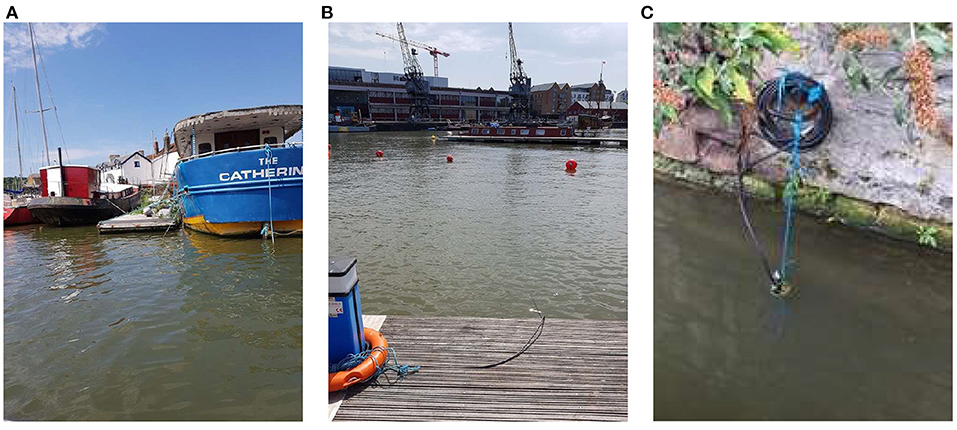
Figure 2. Sensor deployment sites. (A) Baltic Wharf. (B) Watershed. (C) Feeder Canal.

Data Collection

The data used in this study was collected using three EXO2 water quality sondes from YSI Inc. These are multiparameter sondes equipped with up to seven sensors capable of measuring a wide range of variables (YSI, 2019), found to be largely successful in the field by other researchers (Snazelle, 2015; Snyder et al., 2018). For the purposes of this study, turbidity, fDOM (fluorescent dissolved organic matter, a surrogate for dissolved organic content), conductivity, temperature, and dissolved oxygen (DO) were considered sufficient to capture changes in the harbour due to weather, pollutant, and tidal stimuli.

Data from the three monitoring sites were collected continuously between 2018 and 2020, with occasional interruptions due to calibration of the sensors, loss of battery and sensor's failures. At each site, data was taken every 5 min (0.0033 Hz), with the aim of finding an adequate monitoring frequency lower than this for each variable. The three datasets obtained from the data collection are presented in Table 3.

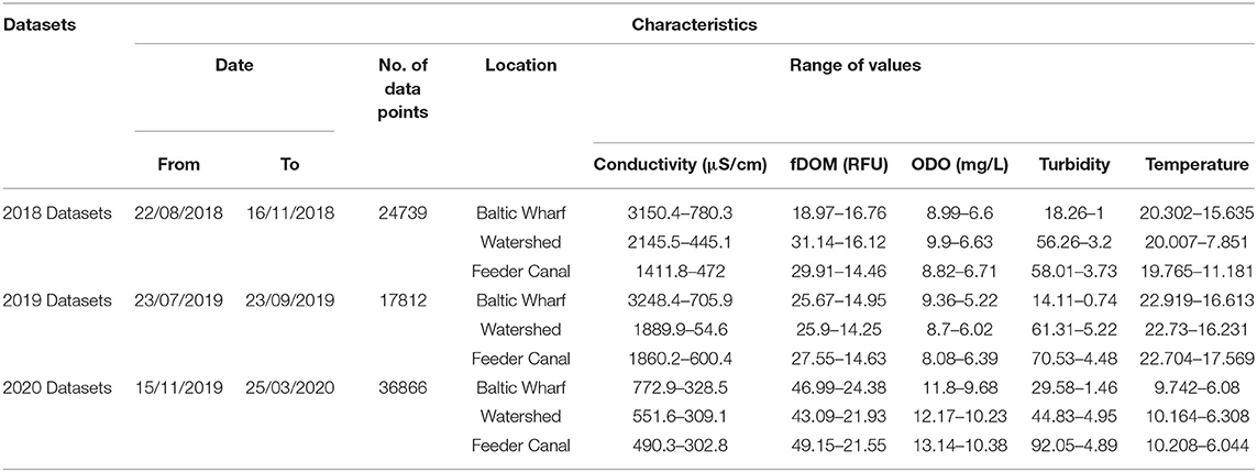
Table 3. Dataset characteristics.

Frequency Analysis

Many signals within water quality parameters exhibit cyclic variability. These are commonly found to have annual, weekly, or diurnal variation. For example, DO and temperature commonly exhibit diurnal variability whereas a location immediately downstream of a dam or sewage treatment plant may exhibit weekly cycles due to reduced water and power usage at weekends (Khalil and Ouarda, 2009). Given this, adequately representing the periodicity of signals of water quality parameters could reflect the worst and best values on the required scale (diurnally, seasonally etc.). Hence, sampling frequency is a very important aspect of water quality monitoring networks. The following subsections describe the three quantitative methods that have been used in this paper to define a procedure to establish the appropriate sampling frequency for water quality parameters to be used when designing a high frequency monitoring quality network.

Harmonic Analysis

Zhou (1996) defines the minimum sampling frequency to achieve this in terms of harmonic analysis. A historical time series can be transformed using Fast Fourier Transform (FFT) from the time domain into frequency domain.

The Fast Fourier Transform is an algorithm that computes the discrete Fourier transform which is obtained by decomposing a sequence of values into components of different frequencies.

The FFT amplitude spectra equation is defined as:

For a timeseries sampled at a given constant interval Δt, harmonics can be observed at frequencies from 0 to 1/(2Δt), where the frequency 1/(2Δt) is known as Nyquist frequency (fn). The Nyquist frequency is the minimum sampling frequency that will allow to truly represent a signal. Thus, fn gives the minimum sampling frequency required (Khalil and Ouarda, 2009). Any harmonics at higher frequencies than fn fold into the signal to appear at lower frequencies. This is known as aliasing and can be avoided by selecting a sufficient minimum sampling rate to capture the highest frequency significant periodic fluctuations in the signal. For a signal with a frequency of the highest significant harmonic f_H, the minimum sampling frequency to avoid aliasing f_S,min = 2f_H (Rorabaugh, 1986; Zhou, 1996).

In this paper, the frequencies f_H− and f_S,min are obtained for each signal using Python. The first step is to determine if there is a trend in the data. If a trend is detected it should be removed before obtaining the frequency amplitude spectra using the fast Fourier transform. From the amplitude spectra, the highest frequency harmonics are identified to find the minimum required sampling rate.

Spectral Analysis—Power Spectral Density

Decomposing the timeseries into a sum of weighted sinusoids allows to assess the frequency content of the signal analysed. Powerful tools such as spectral analysis allow to determine the importance of each frequency. The water quality parameter signal can be concentrated in some narrow frequency band, or it may be spread across a broad range of frequencies.

da Silva et al. (2019) in their study used spectral analysis to evaluate the representativeness of water quality sampling frequencies for different catchments. In particular, the representation of the spectral coefficients of a signal as a function of frequency results in a graph of frequency densities, which is also called Power Spectral Density (PSD).

The purpose of computing PSD analysis is to see how the frequency content of the signal varies with the frequency and how, after a certain frequency, the PSD reach a steady point. This means that after a certain point with an increase in the frequency there won't be an increase in the information collected.

In this study the PSD has been computed with the Welch's method according to Otis and Solomon (1991).

Welch's method (also called the periodogram averaging method) for estimating power spectra is carried out by dividing the time signal into successive segments or blocks, forming the periodogram for each block, and averaging. The computation is described in the following steps:

1) The data sequence is divided into K segments:

where: M = Number of points in each segment

S = Number of points to shift between each segment

K = Number of segments.

2) The windowed discrete Fourier transform is computed for each segment at a frequency

3) For each segment, the modified periodogram value [P_k(f)] is obtained from the discrete Fourier Transform:

Where:

4) Averaging the periodogram values, the Welch's estimate of the PSD will be obtained:

In other words, the PSD it's just an average of periodograms across time and describe how the power of a signal is distributed over frequency.

After obtaining the power spectral density for each parameter at each monitoring station, the worst-case scenario has been analysed. The curve containing the lowest power for each frequency has been selected and the accumulation curve of the PSD has been calculated:

After the accumulation, the values have been replaced by relative values (percentage of the total accumulated in each curve) to normalise all the curves.

These curves have been used to determine the sampling intervals for each cumulated density. In each of these curves the frequency values corresponding to the cumulated PSD were extracted from 10 to 90% in increments of 10% and elbow points were found using the Kneedle Python library. The Kneedle algorithm detects those beneficial data points that identify the maximum curvature and capture the levelling off effect. These points are called “knees” and they are calculated in discrete data sets based on the mathematical definition of curvature for continuous functions (Satopää et al., 2011).

This algorithm has been used to detect the point on the PSD curve after which the amount of information collected increases at a slower rate.

Wavelet Analysis

The Wavelet transforms are mathematical techniques that use analysing functions, localised in space, called wavelets. Unlike the Fourier transform, that can only give precise information on the frequency spectrum of the signal, wavelet analysis can give information on both time and frequency; it sacrifices frequency precision but gains temporal information.

Choosing between different wavelet shape it's possible to find the one that fits best with the feature of the signal that will be analysed.

For the purpose of this paper, the Morlet wavelet has been selected as “mother wavelet” and it's defined as:

The Continuous Wavelet Transform (CWT) can be described by the following equation:

The scale factor corresponds to how much a signal is scaled in time and it is inversely proportional to frequency. This means that the higher the scale, the finer the scale discretion.

The different wavelets in scales and time are shifted along the entire signal and multiplied by its sampling interval to obtain physical significances, resulting in coefficients that are a function of wavelet scales and shift parameters.

In this study we applied the CWT to the non-stationary signal and we visualised the resulting coefficient in a scalogram using the Waipy Python library based on Torrence and Compo (1998).

Results

Nyquist Frequencies

The frequency analysis applied to the time series of temperature, dissolved oxygen (ODO), and fDOM has shown that the sampling interval to adequately characterise the water body should be at least 6 h (see Figure 3).

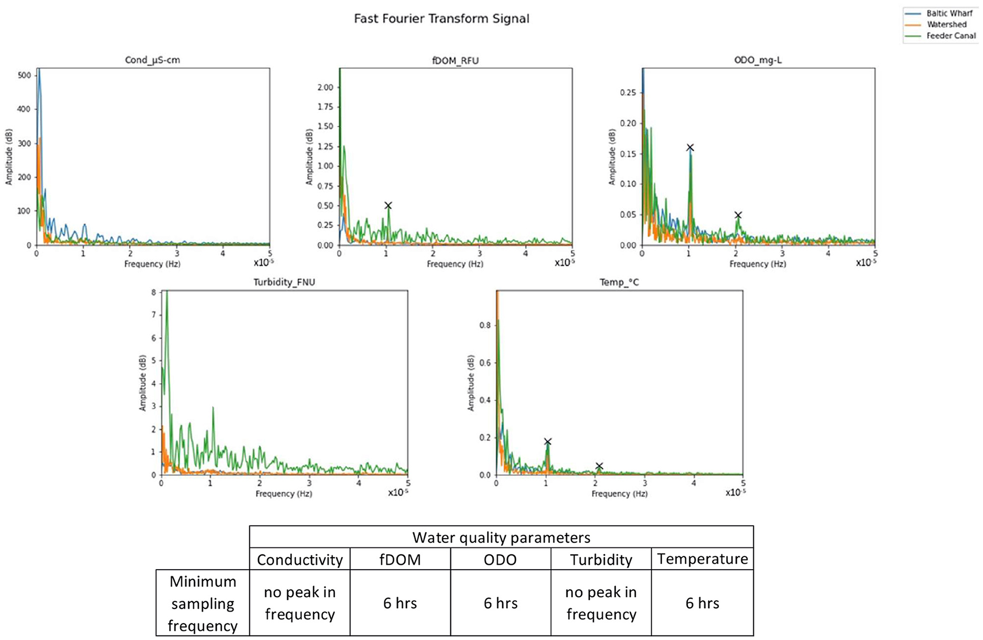
Figure 3. Fast Fourier transform signal for the monitored parameters at 3 different locations. The marked peaks represent the minimum sampling frequencies. The values of the minimum sampling frequency marked on the plots are shown in the table.

The water temperature sampling intervals resulted as 12 and 6 h intervals were expected since water temperature vary in response to diurnal and seasonal changes in solar radiation.

Similar results are obtained for the dissolved oxygen since it is highly dependent on temperature and salinity. In the Floating Harbour dissolved oxygen is mainly affected by temperature changes since levels of salinity are quite low compared to sea water so the effect of changes in salinity on dissolved oxygen is negligible.

The dissolved organic matter is measuring the fDOM (fluorescent dissolved organic matter), a fraction of CDOM that fluoresces when it absorbs light of a certain spectrum. The CDOM (coloured dissolved organic matter) is a naturally occurring dissolved matter that absorbs UV light in water. It is usually material that is released from the breakdown of plant material. The observed values for fDOM in the Floating Harbour vary significantly in the three different sites due to different landscape characteristics, also showing a diurnal change due to the important influence of solar radiation on the measurements.

For the turbidity measurements there is no constant periodicity in the recorded time series, resulting in noisy frequency spectrum. This shows that turbidity in the Floating Harbour is not controlled by a cyclic phenomenon but by external forces. It was unexpected that the scouring operations happening in the harbour did not have an immediate effect on the turbidity measurements. This might be because the sites chosen for the deployment of sensors were not reached by the main flow during scouring operations.

The conductivity signal doesn't show frequency peaks but the conductivity timeseries show a high correlation to the tide affecting the Bristol Channel and River Avon. Concluding that the tides are primarily responsible for the cyclic variation of conductivity in the Floating Harbour, a monitoring frequency must be high enough to capture the extreme levels of conductivity caused by the tidal water entering the harbour. As very high tides are not strictly periodic in time, the harmonic analysis is not completely applicable.

Power Spectral Density Cumulation Plots

From the harmonic analysis it has been possible to find the minimum required sampling frequency for some of the parameters, but it has not been possible to verify which frequencies have the highest density in the signal.

The PSD cumulation curve is the integration of the PSD function. It allows us to assess at specific sampling frequencies how representative would be the sampling and vice versa. Figure 4 is an example of the percentage of signal that is recorded at different frequencies for different parameters. The curve represents the worst-case curve among the different sampling locations. The PSD curves, after a certain frequency, reach a steady point. This means that with an increase in the frequency there won't be an increase in the information collected. Parameters that have recurrent paths (i.e., temperature, conductivity, and dissolved oxygen) reach the steady point quicker than the ones that don't show strong periodicity.

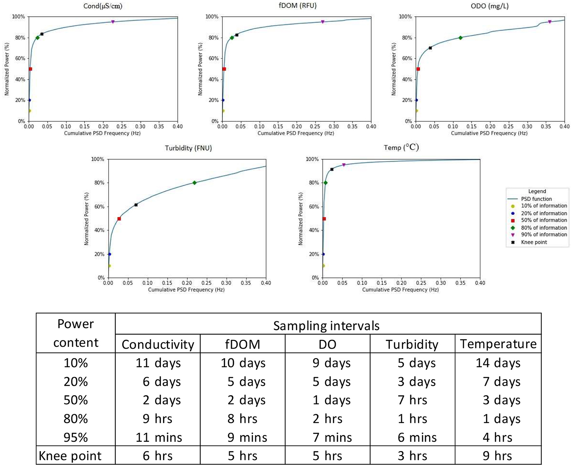
Figure 4. Cumulation PSD plots using the worst-case scenario dataset. The values for the points marked on the plots are shown in the table. The accumulated frequency shows the quantity of information that will be collected with a specific sampling interval for a water quality parameter.

Wavelet Transform

Timeseries give precise information on the amplitude of the signal changing with time but don't give information on the frequency spectrum of the signal. The spectral analysis instead can evaluate the size of the component of the frequencies but gives no information on spatial duration. When it comes to parameters that don't have fixed fluctuations it's important to be able to link the time to the frequency domain in order to understand their pattern. In the spectrograms obtained from the Wavelet analysis, each wavelet measurement (the wavelet transform corresponding to a fixed parameter) tells something about the temporal extent of the signal, as well as something about the frequency spectrum of the signal.

The scalograms containing the results of the Wavelet transform (Figures 5, 6) display the frequency the period scale on the y-axis, and their prevalence on the x-axis. The wavelet scale (the power) is represented at the bottom of the plot. The cone shaped line is the cone of impact (COI), an area where the wavelet power spectra are distorted due to the influence of the end points of finite-length signals. Peaks within these regions have been reduced in magnitude (Torrence and Compo, 1998).

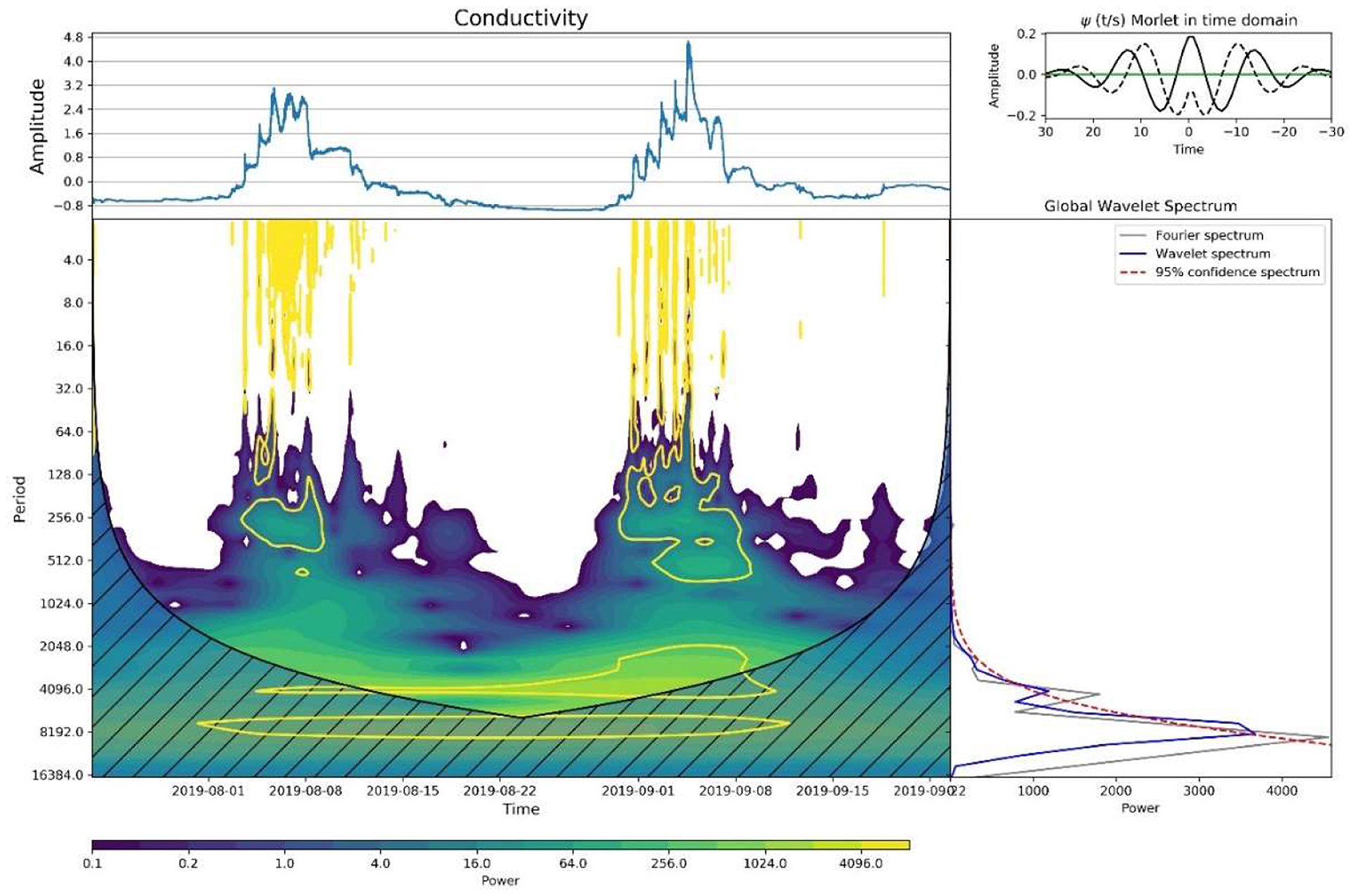
Figure 5. Wavelet analysis – conductivity.

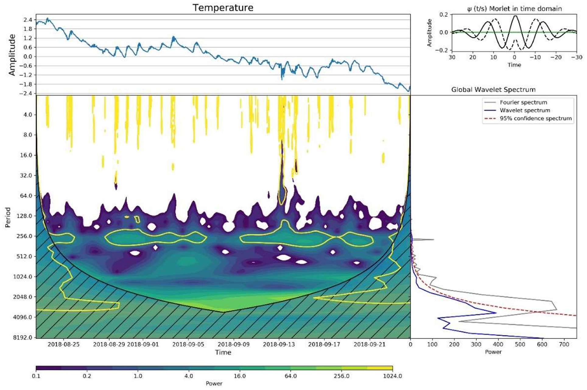
Figure 6. Wavelet analysis – temperature.

From Figure 5 it is possible to see that the sampling frequency changes with time, in this case when peaks in the conductivity timeseries occur the sampling frequency required is higher compared to periods where the conductivity is stable. Therefore, for conductivity measurements it is not accurate to define one sampling frequency constant in time. The sampling frequency should be linked to the tide measurements. A low frequency/low tide—high frequency/high tide sampling frequency should be defined. This sampling scheme will better represent the conductivity peaks and avoid oversampling in the time windows when the tide is not entering the Floating Harbour.

Figure 6 shows how diurnal variation of water quality parameter can easily be identified using Wavelet analysis. To be able to catch the presence of daily pattern a high required sampling frequency is needed according to the PSD analysis.

From the Wavelet analysis it's possible to see that measuring at a sampling frequency lower than the one suggested by the PSD analysis, although will miss the daily variations, will still show the overall trend creating a good compromise between sampling frequency and information collected.

Discussion and Conclusions

This study investigated the sampling frequency required to communicate periodic fluctuations in various water quality parameters and evaluated the benefit of recording data at higher frequencies while considering external factors. The results can be used to match sampling frequency with the purpose of the monitoring programme so that the accuracy is adequate to achieve the purpose. We consider three broad purposes for monitoring: understanding long term baselines and trends, understanding events and providing input to models and in particular machine learning applications.

Using the time series of water quality data available in Bristol Floating Harbour the frequency components of each water quality parameter has been analysed to quantify the Nyquist frequency and the supposed minimum sampling rate for determination of periodic fluctuations, as proposed by Zhou (1996) and Khalil and Ouarda (2009). For most of the monitored water quality parameters it has been possible to identify minimum frequencies that can be used in cases where there are constraints on data storage and handling, providing a means for robustly defending the sampling frequency in the design of the WQMN.

Designing a WQMN with a frequency equal to the minimum sampling frequency is useful if the network is set up for event based monitoring. For this purpose there is no need to have a real-time WQMN set up in advance and grab sampling would perform well.

When designing a WQMN with the purpose of monitoring long term trends and baselines the minimum sampling frequency can also be used with the advantage of minimising data storage.

The minimum sampling frequency approach is not a suitable choice if the purpose of the WQMN is providing input to models, higher frequency data is needed to ensure the accuracy of the model.

Using the PSD function, it has been possible to determine which frequencies have the highest density in the signal, therefore, how representative of the overall situation a particular frequency will be. The PSD cumulation curve showed that after a certain point, increasing the frequency does not deliver an increase in information gained, allowing to find the compromise between having enough data to fully characterise the variability in water quality while not overwhelming the databases. This point is identified by finding the maximum curvature of the PSD cumulative function also called the Knee point.

In this paper it is demonstrated that the frequency corresponding to the PSD function knee point supports the results obtained with harmonic analysis.

One of the main advantages of this method over the harmonic analysis is that it has been possible to define an optimum sampling frequency for parameters that do not show periodicity such as conductivity and turbidity. Although there is a mathematical function that defines the optimum sampling frequency, when defining the optimum frequency it is also important to consider the main purpose of the monitoring network, financial resources and data storage capabilities.

In particular, the results obtained with the PSD function give precious information for designing a WQMN with the purpose of collecting input data for machine learning models. In these models having a high accuracy in the input data helps with achieving a good overall performance of the model.

High frequency data comes with the need to have a real-time monitoring network set up in specific locations, this puts limits on the flexibility of the purpose of the network and on the network itself. For this reason high frequency data collection is less suitable for event based monitoring where flexibility is important.

To have a complete understand of the optimum frequencies obtained with the PSD analysis and to tailor them to the purpose of the network it is important to look at the timeseries as well as at the frequency spectra.

The problem of losing time localisation in the spectral analysis is mitigated by the use of a wavelet analysis. The Wavelet analysis gives information on both the amplitude of the signal and the frequency spectrum. In this paper the spectrogram of the wavelet analysis has been used qualitatively. Looking at the spectrograms it is possible to gain extra information on parameters that do not have constant periodicity and it is possible to better tailor the frequency interval to the purpose of the sampling network.

Estimating sampling frequency according to the accuracy needed in the WQMN, allows for the optimization of monitoring methodologies and improvement in decision-making and regulatory development. Quality-assurance protocols are implemented by water-monitoring agencies to reduce overall uncertainty; however, sampling precision estimations were previously under-quantified or overlooked due to lack of high-frequency data with which to compare sample estimates. Many previous studies have noted the substantial errors that result from sampling frequency that were not representative of the actual water quality parameter trends; this was mostly due to lack of continuous and high frequency datasets (Jones et al., 2014; Reynolds et al., 2016).

Although results of this study would provide the stakeholders with the optimum sampling frequency needed to get most accurate water quality trends, this may not be economically feasible in long terms or for large-scale applications. Understanding the marginal return on sampling effort will lead to obtain more useful information and adjust sampling strategy or frequency to balance effort and accuracy. Further investigations flowing from these findings include:

- Exploring spatial variability of sampling locations and its effect on sampling frequency.

- Understanding how the proposed techniques can be used for event based monitoring and also investigating how to filter out the effects of events on baseline water quality.

- Defining a statistical method to link the sampling frequency to a specific WQMN purpose.

- Evaluating the impact of the sampling frequency on the noise in the data. This could be done by comparing higher and lower frequency datasets for the same parameter/period.

Data Availability Statement

The raw data supporting the conclusions of this article will be made available by the authors, without undue reservation.

Author Contributions

EC carried out data collection, data analysis, and wrote the paper. DH provided guidance. CG and TT provided advice on the manuscript enhancement. All authors contributed to the article and approved the submitted version.

Funding

This work was funded as part of the Water Informatics Science and Engineering Centre for Doctoral Training (WISE CDT) under a grant from the Engineering and Physical Sciences Research Council (EPSRC), grant number EP/L016214/1. This work was supported in part by the Engineering and Physical Sciences Research Council's (ESPRC) UK Collaboratorium for Research in Infrastructure & Cities (UKCRIC): Urban Observatories grant (ref. EP/P016782/1).

Conflict of Interest

The authors declare that the research was conducted in the absence of any commercial or financial relationships that could be construed as a potential conflict of interest.

Publisher's Note

All claims expressed in this article are solely those of the authors and do not necessarily represent those of their affiliated organizations, or those of the publisher, the editors and the reviewers. Any product that may be evaluated in this article, or claim that may be made by its manufacturer, is not guaranteed or endorsed by the publisher.

Acknowledgments

Many thanks to Bristol City Council's Harbour Master's office for their kind aid in deploying the sensors in the harbour and to Dr. Yiheng Chen that helped with the data collection.

References

Anvari, A., Delos Reyes, J., Esmaeilzadeh, E., Jarvandi, A., Langley, N., and Navia, K. R. (2009). “Designing an automated water quality monitoring system for West and Rhode Rivers,” in Systems and Information Engineering Design Symposium (Charlottesville, VA: IEEE). doi: 10.1109/SIEDS.2009.5166167
Bartram, J., and Ballance, R. (1996). Water Quality Monitoring: A Practical Guide to the Design and Implementation of Frewshwater Quality Studies and Monitoring Programmes. London: E & FN SPON.
Behmel, S., Damour, M., Ludwig, R., and Rodriguez, M. J. (2016). Water quality monitoring strategies - A review and future perspectives. Sci. Total Environ. 571, 1312–1329. doi: 10.1016/j.scitotenv.2016.06.235
Birgand, F., Appelboom, T. W., Chescheir, G. M., and Skaggs, R. W. (2013). Estimating nitrogen, phosphorus, and carbon fluxes in forested and mixed-use watersheds of the lower coastal plain of North Carolina: uncertainties associated with infrequent sampling. Transact. ASABE 54, 2099–2110. doi: 10.13031/2013.40668
Bristol City Council (2006). Bristol Floating Harbour Recreational Water Profile. Bristol. Available online at: https://www.bristol.gov.uk/documents/20182/32707/Harbour%20Water%20Profile%202013.pdf/7984ce98-8830-4f19-9f4f-fe7fc233b734 (accessed April 26, 2019).
Bristol City Council (2013). Bristol Floating Harbour Recreational Water Profile. Available online at: https://www.bristol.gov.uk/documents/20182/32707/HarbourWaterProfile%202013.pdf/7984ce98-8830-4f19-9f4f-fe7fc233b734 (accessed October 4, 2021).
Chappell, N. A., Jones, T. D., and Tych, W. (2017). Sampling frequency for water quality variables in streams: Systems analysis to quantify minimum monitoring rates. Water Res. 123, 49–57. doi: 10.1016/j.watres.2017.06.047
Chen, Y., and Han, D. (2018). Water quality monitoring in smart city: A pilot project. Automation Const. 89, 307–316. doi: 10.1016/j.autcon.2018.02.008
da Silva, R. L. L., da Silveira, A. L. L., and da Silveira, G. L. (2019). Spectral analysis in determining water quality sampling intervals. Rev. Brasil. Recursos Hidricos 24:80077. doi: 10.1590/2318-0331.241920180077
Guigues, N., Desenfant, M., and Hance, E. (2013). Combining multivariate statistics and analysis of variance to redesign a water quality monitoring network. Environ. Sci. 15, 1692–1705. doi: 10.1039/c3em00168g
Hadimani, P. S., Mane, S. B., Korvi, R. S., and Saurabh, P. R. (2021). IOT based water quality monitoring system. Int. J. Sci. Res. Eng. Trends 7, 2395–2566. Available online at: https://ijsret.com/wp-content/uploads/2021/05/IJSRET_V7_issue3_370.pdf
Halliday, S. J., Skeffington, R. A., Wade, A. J., Bowes, M. J., Gozzard, E., Newman, J. R., et al. (2015). High-frequency water quality monitoring in an urban catchment: hydrochemical dynamics, primary production and implications for the Water Framework Directive. Hydrol. Process. 29, 3388–3407. doi: 10.1002/hyp.10453
Ivanovsky, A., Criquet, J., Dumoulin, D., Alary, C., Prygiel, J., Duponchel, L., et al. (2016). Water quality assessment of a small peri-urban river using low and high frequency monitoring. Environ. Sci. 18, 624–637. doi: 10.1039/C5EM00659G
Jiang, J., Tang, S., Han, D., Fu, G., Solomatine, D., and Zheng, Y. (2020). A comprehensive review on the design and optimization of surface water quality monitoring networks. Environ. Model. Software 132:104792. doi: 10.1016/j.envsoft.2020.104792
Jones, T., Chappell, N. A., and Tych, W. (2014). First dynamic model of dissolved organic carbon derived directly from high frequency observations through contiguous storms. Environ. Sci. Technol. 48, 13289–13297. doi: 10.1021/es503506m
Khalil, B., Ou, C., Proulx-McInnis, S., St-Hilaire, A., and Zanacic, E. (2014). Statistical Assessment of the Surface Water Quality Monitoring Network in Saskatchewan. Water, Air, & Soil Pollution 225, 1–22. doi: 10.1007/s11270-014-2128-1
Khalil, B., and Ouarda, T. B. M. J. (2009). Statistical approaches used to assess and redesign surface water-quality-monitoring networks. J. Environ. Monitor. 2009, 1915–1929. doi: 10.1039/b909521g
Kirchner, J. W., Feng, X., Neal, C., and Robson, A. J. (2004). The fine structure of water-quality dynamics: The (high-frequency) wave of the future. Hydrol. Process. 18, 1353–1359. doi: 10.1002/hyp.5537
Liu, Y., Zheng, B., Wang, M., Xu, Y., and Qin, Y. (2013). Optimization of sampling frequency for routine river water quality monitoring. Sci. China Chem. 57, 772–778. doi: 10.1007/s11426-013-4968-8
Marcé, R., George, G., Buscarinu, P., Deidda, M., Dunalska, J., De Eyto, E., et al. (2016). Automatic high frequency monitoring for improved lake and reservoir management. Environ. Sci. Technol. 50, 10780–10794. doi: 10.1021/acs.est.6b01604
Naddeo, V., Zarra, T., and Belgiorno, V. (2007). Optimization of sampling frequency for river water quality assessment according to Italian implementation of the EU Water Framework Directive. Environ. Sci. Policy 10, 243–249. doi: 10.1016/j.envsci.2006.12.003
Nguyen, T. H., Helm, B., Hettiarachchi, H., Caucci, S., and Krebs, P. (2019). The selection of design methods for river water quality monitoring networks: a review. Environ. Earth Sci. 75:321. doi: 10.1007/s12665-019-8110-x
Ordnance Survey (2019). 1:25000 Scale Colour Raster'. Ordnance Survey (GB), Using: EDINA Digimap Ordnance Survey Service.
Otis, M., and Solomon, J. (1991). PSD Computations Using Welch's Method. Available online at: https://www.osti.gov/servlets/purl/5688766 (accessed September 16, 2021).
Reynolds, K. N., Loecke, T. D., Burgin, A. J., Davis, C. A., Riveros-Iregui, D., Thomas, S. A., et al. (2016). Optimizing sampling strategies for riverine nitrate using high-frequency data in agricultural watersheds. Environ. Sci. Technol. 50, 6406–6414. doi: 10.1021/acs.est.5b05423
Satopää, V., Albrecht, J., Irwin, D., and Raghavan, B. (2011). “Finding a “Kneedle” in a haystack: detecting knee points in system behavior,” in Notes Proceedings of the 30th International Conference on Distributed Computing Systems SIMPLEX Workshop (Minneapolis, MN). doi: 10.1109/ICDCSW.2011.20
Skeffington, R. A., Halliday, S. J., Wade, A. J., Bowes, M. J., and Loewenthal, M. (2015). Using high-frequency water quality data to assess sampling strategies for the EU Water Framework Directive. Hydrol. Earth Syst. Sci 19, 2491–2504. doi: 10.5194/hess-19-2491-2015
Snazelle, T. T. (2015). Evaluation of Xylem EXO Water-Quality Sondes and Sensors: U.S. Geological Survey open-File Report 2015–1063, 28. doi: 10.3133/ofr20151063
Snyder, L., Potter, J. D., and McDowell, W. H. (2018). An evaluation of nitrate, fDOM, and turbidity sensors in new hampshire streams. Water Resour. Res. 54, 2466–2479. doi: 10.1002/2017WR020678
Strobl, R. O., and Robillard, P. D. (2008). Network design for water quality monitoring of surface freshwaters: A review. J. Environ. Manage. 87, 639–648. doi: 10.1016/j.jenvman.2007.03.001
Tapparello, C., Abdulai, J. D., Katsriku, F. A., Heinzelman, W., and Adu-Manu, K. S. (2017). Water quality monitoring using wireless sensor networks. ACM Transact. Sensor Networks 13, 1–41. doi: 10.1145/3005719
Torrence, C., and Compo, G. (1998). A Practical Guide to Wavelet Analysis in: Bulletin of the American Meteorological Society. American Meteriology Society. Available online at: https://journals.ametsoc.org/view/journals/bams/79/1/1520-0477_1998_079_0061_apgtwa_2_0_co_2.xml (accessed September 16, 2021).
Zhou, C., Zhang, C., Tian, D., Wang, K., Huang, M., and Liu, Y. (2018). A software sensor model based on hybrid fuzzy neural network for rapid estimation water quality in Guangzhou section of Pearl River, China. J. Environ. Sci. Health Part A 53, 91–98. doi: 10.1080/10934529.2017.1369815
Keywords: sampling frequency, water quality, monitoring network design, high frequency data analysis, wireless sensor network (WSN)
Citation: Coraggio E, Han D, Gronow C and Tryfonas T (2022) Water Quality Sampling Frequency Analysis of Surface Freshwater: A Case Study on Bristol Floating Harbour. Front. Sustain. Cities 3:791595. doi: 10.3389/frsc.2021.791595
Received: 08 October 2021; Accepted: 21 December 2021;
Published: 31 January 2022.
Edited by:
James Evans, The University of Manchester, United KingdomReviewed by:
Prashant Rajput, Banaras Hindu University, IndiaTomiwa Sunday Adebayo, Cyprus International University, Cyprus
Copyright © 2022 Coraggio, Han, Gronow and Tryfonas. This is an open-access article distributed under the terms of the Creative Commons Attribution License (CC BY). The use, distribution or reproduction in other forums is permitted, provided the original author(s) and the copyright owner(s) are credited and that the original publication in this journal is cited, in accordance with accepted academic practice. No use, distribution or reproduction is permitted which does not comply with these terms.
*Correspondence: Elisa Coraggio, elisa.coraggio@bristol.ac.uk