A Mathematical Formalization of Hierarchical Temporal Memory’s Spatial Pooler
 James Mnatzaganian
 Ernest Fokoué
 Dhireesha Kudithipudi1
- 1NanoComputing Research Laboratory, Computer Engineering Department, Kate Gleason College of Engineering, Rochester Institute of Technology, Rochester, NY, USA
- 2Data Science Research Group, School of Mathematical Sciences, College of Science, Rochester Institute of Technology, Rochester, NY, USA
Hierarchical temporal memory (HTM) is an emerging machine learning algorithm, with the potential to provide a means to perform predictions on spatiotemporal data. The algorithm, inspired by the neocortex, currently does not have a comprehensive mathematical framework. This work brings together all aspects of the spatial pooler (SP), a critical learning component in HTM, under a single unifying framework. The primary learning mechanism is explored, where a maximum likelihood estimator for determining the degree of permanence update is proposed. The boosting mechanisms are studied and found to be a secondary learning mechanism. The SP is demonstrated in both spatial and categorical multi-class classification, where the SP is found to perform exceptionally well on categorical data. Observations are made relating HTM to well-known algorithms such as competitive learning and attribute bagging. Methods are provided for using the SP for classification as well as dimensionality reduction. Empirical evidence verifies that given the proper parameterizations, the SP may be used for feature learning.
1. Introduction
Hierarchical temporal memory (HTM), created by Hawkins and George (2007), is a machine learning algorithm that was inspired by the neocortex and designed to learn sequences and make predictions. In its idealized form, it should be able to produce generalized representations for similar inputs. Given time-series data, HTM should be able to use its learned representations to perform a type of time-dependent regression. Such a system would prove to be incredibly useful in many applications utilizing spatiotemporal data. One instance for using HTM with time-series data was recently demonstrated by Cui et al. (2016), where HTM was used to predict taxi passenger counts. Lavin and Ahmad (2015), additionally, used HTM for anomaly detection. HTM’s prominence in the machine learning community has been hampered, largely due to the evolving nature of HTM’s algorithmic definition and the lack of a formalized mathematical model. This work aims to bridge the gap between a neuroscience inspired algorithm and a math-based algorithm by constructing a purely mathematical framework around HTM’s original algorithmic definition.
HTM models at a high-level, some of the structures and functionality of the neocortex. Its structure follows that of the cortical minicolumns, where an HTM region is comprised of many columns, each consisting of multiple cells. One or more regions form a level. Levels are stacked hierarchically in a tree-like structure to form the full network depicted in Figure 1. Within HTM, connections are made via synapses, where both proximal and distal synapses are utilized to form feedforward and neighboring connections, respectively.
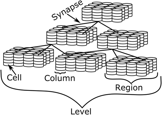
Figure 1. Depiction of HTM, showing the various levels of detail.
The current version of HTM is the successor to HTM cortical learning algorithm (Hawkins et al., 2011). In the current version of HTM, the two primary algorithms are the spatial pooler (SP) and the temporal memory (TM). The SP is responsible for taking an input, in the format of a sparse distributed representation (SDR), and producing a new SDR, where an SDR is a binary vector typically having a sparse number of active bits, i.e., a bit with a value of “1” (Ahmad and Hawkins, 2015). In this manner, the SP can be viewed as a mapping function from the input domain to a new feature domain. In the feature domain, a single SDR should be used to represent similar SDRs from the input domain. The algorithm is a type of unsupervised competitive learning algorithm (Rumelhart and Zipser, 1985) that uses a form of vector quantization (Gersho and Gray, 2012) resembling self-organizing maps (Kohonen, 1982). The TM is responsible for learning sequences and making predictions. This algorithm follows Hebb’s rule (Hebb, 1949), where connections are formed between cells that were previously active. Through the formation of those connections, a sequence may be learned. The TM can then use its learned knowledge of the sequences to form predictions.
HTM originated as an abstraction of the neocortex; as such, it does not have an explicit mathematical formulation. Without a mathematical framework, it is difficult to understand the key characteristics of the algorithm and how it can be improved. In general, very little work exists regarding the mathematics behind HTM. Hawkins and Ahmad (2016) recently provided a starting mathematical formulation for the TM. Ahmad and Hawkins (2015) additionally provided some initial formalizations for the SP. Lattner (2014) provided an initial insight about the SP, by relating it to vector quantization. He additionally provided some equations governing computing overlap and performing learning; however, those equations were not generalized to account for local inhibition. Byrne (2015) began the use of matrix notation and provided a basis for those equations; however, certain components of the algorithm, such as boosting, were not included. Leake et al. (2015) provided some insights regarding the initialization of the SP. He also provided further insights into how the initialization may affect the initial calculations within the network; however, his focus was largely on the network initialization. The goal of this work is to provide a complete mathematical framework for HTM’s SP and to demonstrate how it may be used in various machine learning tasks. Having a mathematical framework creates a basis for future algorithmic improvements, allows for a more efficient software implementation, and eases the path for hardware engineers to develop scalable HTM hardware.
The major, novel contributions provided by this work are as follows:
• Creation of a complete mathematical framework for the SP, including boosting and local inhibition.
• Using the SP to perform feature learning.
• Using the SP as a preprocessor for non-spatial (categorical) data.
• Creation of a possible mathematical explanation for the permanence update amount.
• Insights into the permanence selection.
2. Spatial Pooler Algorithm
The SP consists of three phases, namely overlap, inhibition, and learning. In this section, the three phases will be presented based off their original, algorithmic definition. This algorithm follows an iterative, online approach, where the learning updates occur after the presentation of each input. Before the execution of the algorithm, some initializations must take place.
Within an SP, there exist many columns. Each column has a unique set of proximal synapses connected via a proximal dendrite segment. Each proximal synapse tentatively connects to a single column from the input, i.e., each column in the SP connects to a specific attribute within the input. The input column’s activity level is used as the synaptic input, i.e., an active column is a “1” and an inactive column is a “0”.
To determine whether a synapse is connected or not, the synapse’s permanence value is checked. If the permanence value is at least equal to the connected threshold the synapse is connected; otherwise, it is unconnected. The permanence values are scalars in the closed interval [0, 1].
Prior to the first execution of the algorithm, the potential connections of proximal synapses to the input space and the initial permanence values must be determined. Following Hawkins et al. (2011), each synapse is randomly connected to a unique attribute in the input, i.e., the number of synapses per column and the number of attributes are binomial coefficients. The permanences of the synapses are then randomly initialized to a value close to the connected permanence threshold. The permanences are then adjusted such that shorter distances between the SP column’s position and the input column’s position will result in larger initial permanence values. The three phases of the SP are explained in the following subsections.
2.1. Phase 1: Overlap
The first phase of the SP is used to compute the overlap between each column and its respective input, as shown in Algorithm 1. In Algorithm 1, the SP is represented by the object sp. The method col.connected_synapses() returns an instance to each synapse on col’s proximal segment that is connected, i.e., synapses having permanence values greater than the permanence connected threshold, psyn_th. The method syn.active() returns “1” if syn’s input is active and “0” otherwise. pseg_th1 is a parameter that determines the activation threshold of a proximal segment, such that there must be at least pseg_th active connected proximal synapses on a given proximal segment for it to become active. The parameter col.boost is the boost value for col, which is initialized to “1”.
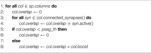
Algorithm 1. SP phase 1: overlap.
2.2. Phase 2: Inhibition
The second phase of the SP is used to compute the set of active columns after they have been inhibited, as shown in Algorithm 2. In Algorithm 2, kmax_overlap(C, k) is a function that returns the k-th largest overlap of the columns in C. The method sp.neighbors(col) returns the columns that are within col’s neighborhood, including col, where the size of the neighborhood is determined by the inhibition radius. The parameter k is the desired column activity level. In line 2 in Algorithm 2, the k-th largest overlap value out of col’s neighborhood is being computed. A column is then said to be active if its overlap value is greater than zero and the computed minimum overlap, mo.
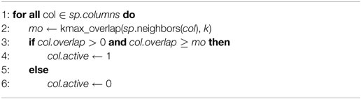
Algorithm 2. SP phase 2: inhibition.
2.3. Phase 3: Learning
The third phase of the SP is used to conduct the learning operations, as shown in Algorithm 3. This code contains three parts – permanence adaptation, boosting operations, and the inhibition radius update. In Algorithm 3, syn.p refers to the permanence value of syn. The functions min and max return the minimum and maximum values of their arguments, respectively, and are used to keep the permanence values bounded in the closed interval [0, 1]. The constants syn.psyn_inc and syn.psyn_dec are the proximal synapse permanence increment and decrement amounts, respectively.
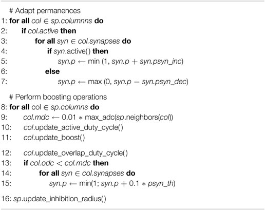
Algorithm 3. SP phase 3: learning.
The function max_adc(C) returns the maximum active duty cycle of the columns in C, where the active duty cycle is a moving average denoting the frequency of column activation. Similarly, the overlap duty cycle is a moving average denoting the frequency of the column’s overlap value being at least equal to the proximal segment activation threshold. The functions col.update_active_duty_cycle() and col.update_overlap_duty_ cycle() are used to update the active and overlap duty cycles, respectively, by computing the new moving averages. The parameters col.odc, col.adc, and col.mdc refer to col’s overlap duty cycle, active duty cycle, and minimum duty cycle, respectively. Those duty cycles are used to ensure that columns have a certain degree of activation.
The method col.update_boost() is used to update the boost for column, col, as shown in Algorithm 4, where maxb refers to the maximum boost value. It is important to note that the whitepaper did not explicitly define how the boost should be computed. This boost function was obtained from the source code of Numenta’s implementation of HTM, Numenta platform for intelligent computing (NuPIC) (Numenta, 2016).
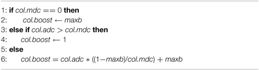
Algorithm 4. Boost update: col.update_boost( ).
The method sp.update_inhibition_radius() is used to update the inhibition radius. The inhibition radius is set to the average receptive field size, which is average distance between all connected synapses and their respective columns in the input and the SP.
3. Mathematical Formalization
The aforementioned operation of the SP lends itself to a vectorized notation. By redefining the operations to work with vectors it is possible not only to create a mathematical representation but also to greatly improve upon the efficiency of the operations. The notation described in this section will be used as the notation for the remainder of the document.
All vectors will be lowercase, bold-faced letters with an arrow hat. Vectors are assumed to be row vectors, such that the transpose of the vector will produce a column vector. All matrices will be uppercase, bold-faced letters. Subscripts on vectors and matrices are used to denote where elements are being indexed, following a row–column convention, such that Xi,j ∈ X refers to X at row index2 i and column index j. Similarly, Xi is a row vector containing all elements in row i. The symbols ⊙ and ⊕ are used to represent element-wise multiplication and addition, respectively. Element-wise operations between a vector and a matrix are performed columnwise, such that .
Let I(k) be defined as the indicator function, such that the function will return 1 if event k is true and 0 otherwise. If the input to this function is a vector of events or a matrix of events, each event will be evaluated independently, with the function returning a vector or matrix of the same size as its input. Any variable with a superscript in parentheses is used to denote the type of that variable. For example, is used to state that the variable is of type y. In the event that an operation has a before and after the states will be denoted using superscripts, such that and will represent the initial and final versions of , respectively.
All of the user-defined parameters are defined in Table 1.3 These are parameters that must be defined before the initialization of the algorithm. All of those parameters are constants. Let the terms s, a, i, j, and k be defined as integer indices. They are henceforth bounded as follows: s ∈ [0, ns), a ∈ [0, na), i ∈ [0, nc), j ∈ [0, nc], and k ∈ [0, nps).
Table 1. User-defined parameters for the SP.
3.1. Initialization
Competitive learning networks typically have each node fully connected to each attribute in the input. The SP follows a different line of logic, posing a new problem concerning the visibility of an input. As previously explained, the subset of input attributes that connect to a particular column are determined randomly. Let be defined as the set of all columns indices, such that is the column’s index at i. Let be defined as the set of attributes for all inputs, such that Us,a is the attribute for input s at index a. Let be the source column indices for each proximal synapse on each column, such that is the source column’s index of ’s proximal synapse at index k. In other words, each refers to a specific index in Us.
Let be defined as vector of events, such that . Therefore, is the event of attribute a connecting to column a, where is defined to be the uniqueness quantification. The probability of a single attribute, Us,a, connecting to a column is the ratio of nps and na, as shown in equation (1).
It is also desired to know the average number of columns an attribute will connect with. To calculate this, let be defined as a vector of random quantities, such that . Therefore, is the count of connections between each attribute and all columns. Recognizing that the probability of a connection forming in nc follows a binomial distribution, the expected number of columns that an attribute will connect to is simply equation (2).
Using equation (1), it is possible to calculate the probability of an attribute never connecting, as shown in equation (3). Since the probabilities are independent, it simply reduces to the product of the probability of an attribute not connecting to a column, taken over all columns. Let , the random variable governing the number of unconnected attributes. From equation (3), the expected number of unobserved attributes may then be trivially obtained as equation (4). Using equations (3) and (2), it is possible to obtain a lower bound for nc and nps, by choosing those parameters such that a certain amount of attribute visibility is obtained. To ensure, with high probability, the observance of all attributes, equation (3) must be sufficiently close to zero. This is obtained by fully connecting the SP columns to the input columns or by having a sufficiently large number of columns. Once that is satisfied, the desired number of times an attribute is observed may be determined by using equation (2).
Once each column has its set of inputs, the permanences must be initialized. As previously stated, permanences were defined to be initialized with a random value close to ρs but biased based off the distance between the synapse’s source (input column) and destination (SP column). To obtain further clarification, NuPIC’s source code (Numenta, 2016) was consulted. It was found that the permanences were randomly initialized, with approximately half of the permanences creating connected proximal synapses and the remaining permanences creating potential (unconnected) proximal synapses. Additionally, to ensure that each column has a fair chance of being selected during inhibition, there are at least ρd connected proximal synapses on each column.
Let be defined as the set of permanences for each column, such that is the set of permanences for the proximal synapses for . Let be defined as a function that will return the maximum value in . Similarly, let be defined as a function that will return the minimum value in . Each is randomly initialized as shown in equation (5), where Unif represents the uniform distribution. Using equation (5), the expected permanence value is ρs; therefore, half of the proximal synapses connected to each column will be initialized in the connected state. This means that ρd should be chosen such that ρd ≤ nps/2 to sufficiently ensure that each column will have a greater than zero probability for becoming active. Additionally, the columns’ inputs must also be taken into consideration, such that ρd should be chosen to be small enough to take into consideration the sparseness in the input.
It is possible to predict, before training, the initial response of the SP to a given input. This insight allows parameters to be crafted in a manner that ensures a desired amount of column activity. Let be defined as the set of inputs for each column, such that Xi is the set of inputs for . Each Xi,k is mapped to a specific Us,a, such that Xi ⊂ Us when nps ≠ na and Xi ⊆ Us otherwise. Let be defined as a matrix of events, such that Ai,k ≡ Xi,k = 1. Ai,k is therefore the event that the attribute connected via proximal synapse k to column i is active. Let be defined as the probability of the attribute connected via proximal synapse k to column i being active. Therefore, is defined to be the probability of any proximal synapse connected to column i being active. Similarly, is defined to be the probability of any proximal synapse on any column being active. The relationship between these probabilities is given in equations (6) and (7).
Let be defined as a vector of random quantities, such that . Therefore, is the number of active proximal synapses on column i. The expected number of active proximal synapses on column i is then given by equation (8). Let , the random variable governing the average number of active proximal synapses on a column. Equation (8) is then generalized to equation (9), the expected number of active proximal synapses for each column. If , it is very unlikely that there will be enough active proximal synapses on a given column for that column to become active. This could result in an insufficient level of column activations, thereby degrading the quality of the SP’s produced output. Therefore, it is recommended to select ρd as a function of the sparseness of the input, such that . Reducing ρd will increase the level of competition among columns; however, it will also increase the probability of including noisy columns, i.e., columns whose synapses’ inputs are connected to attributes within the input that collectively provide little contextual meaning.
Let be defined as a matrix of events, such that . Therefore, is the event that proximal synapse k is active and connected on column i. Let be defined as a vector of random quantities, such that . Therefore, is the count of active and connected proximal synapses for column i. Let , the probability that a proximal synapse is active and connected.4 Following equation (8), the expected number of active connected proximal synapses on column i is given by equation (10).
Let Bin(k; n, p) be defined as the probability mass function (PMF) of a binomial distribution, where k is the number of successes, n is the number of trials, and p is the success probability in each trial. Let , the random variable governing the number of columns having at least ρd active proximal synapses. Let , the random variable governing the number of columns having at least ρd active connected proximal synapses. Let πx and πac be defined as random variables that are equal to the overall mean of and , respectively. The expected number of columns with at least ρd active proximal synapses and the expected number of columns with at least ρd active connected proximal synapses are then given by equations (11) and (12), respectively.
In equation (11), the summation computes the probability of having less than ρd active connected proximal synapses, where the individual probabilities within the summation follow the PMF of a binomial distribution. To obtain the desired probability, the complement of that probability is taken. It is then clear that the mean is nothing more than that probability multiplied by nc. For equation (12), the logic is similar, with the key difference being that the probability of a success is a function of both X and ρs, as it was in equation (10).
3.2. Phase 1: Overlap
Let be defined as the set of boost values for all columns, such that is the boost for . Let , the bit-mask for the proximal synapse’s activations. Therefore, Yi is a row-vector bit-mask, with each “1” representing a connected synapse and each “0” representing an unconnected synapse. In this manner, the connectivity (or lack thereof) for each synapse on each column is obtained. The overlap for all columns, , is defined by equation (13), which is a function of . is the sum of the active connected proximal synapses for all columns and is defined by equation (14).
Comparing these equations with Algorithm 1, it is clear that will have the same value as col.overlap before line five and that the final value of col.overlap will be equal to . To help provide further understanding, a simple example demonstrating the functionality of this phase is shown in Figure 2.
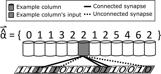
Figure 2. SP phase 1 example where nc = 12, nps = 5, and ρd = 2. It was assumed that the boost for all columns is at the initial value of “1”. For simplicity, only the connections for the example column, highlighted in gray, are shown. The example column’s overlap is two since it has exactly two active and connected synapses.
3.3. Phase 2: Inhibition
Let be defined as the neighborhood mask for all columns, such that Hi is the neighborhood for . is then said to be in ’s neighborhood if and only if Hi,j is “1”. Let kmax(S, k) be defined as the k-th largest element of S. The set of active columns, , is defined by equation (15), such that is an indicator vector representing the activation (or lack of activation) for each column. The result of the indicator function is determined by , which is defined by equation (16) as the ρc-th largest overlap (lower bounded by one) in the neighborhood of .
Comparing these equations with Algorithm 2, is a slightly altered version of mo. Instead of just being the ρc-th largest overlap for each column, it is additionally lower bounded by one. Referring back to Algorithm 2, line 3 is a biconditional statement evaluating to true if the overlap is at least mo and greater than zero. By simply enforcing mo to be at least one, the biconditional is reduced to a single condition. That condition is evaluated within the indicator function; therefore, equation (15) carries out the logic in the if statement in Algorithm 2. Continuing with the demonstration shown in Figures 2 and 3 shows an example execution of phase two.
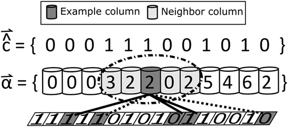
Figure 3. SP phase 2 example where ρc = 2 and the inhibition radius has a size of two. The overlap values were determined from the SP phase 1 example. The ellipse represents the inhibition radius, extending two units in all directions from the example column. The example column is active, because it has an overlap value of two which is at least as large as the ρc-th largest overlap value. It is noted that in this example, within the example column’s inhibition radius, more than ρc columns are active. This situation is valid and occurs when neighboring columns have overlap values that are large enough and close to the example column.
3.4. Phase 3: Learning
Let clip(M, lb, ub) be defined as a function that will clip all values in the matrix M outside of the range [lb, ub] to lb if the value is less than lb, or to ub if the value is greater than ub. Φ is then recalculated by equation (17), where δΦ is the proximal synapse’s permanence update amount given by equation (18).5
The result of these two equations is equivalent to the result of executing the first seven lines in Algorithm 3. If a column is active, it will be denoted as such in ; therefore, using that vector as a mask, the result of equation (18) will be a zero if the column is inactive, otherwise it will be the update amount. From Algorithm 3, the update amount should be ϕ+ if the synapse was active and ϕ− if the synapse was inactive. A synapse is active only if its source column is active. That activation is determined by the corresponding value in X. In this manner, X is also being used as a mask, such that active synapses will result in the update equaling ϕ+ and inactive synapses (selected by inverting X) will result in the update equaling ϕ−. By clipping the element-wise sum of Φ and δΦ, the permanences stay bounded between [0, 1]. As with the previous two phases, the visual demonstration is continued, with Figure 4 illustrating the primary functionality of this phase.
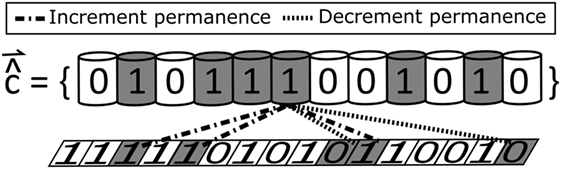
Figure 4. SP phase 3 example, demonstrating the adaptation of the permanences. The gray columns are used to denote the active columns, where those activations were determined from the SP phase 2 example. Permanences are adapted based off the synaptic input for all active columns. If the synaptic input is active, the permanence is incremented otherwise it is decremented.
Let be defined as the set of active duty cycles for all columns, such that is the active duty cycle for . Let be defined by equation (19) as the set of minimum active duty cycles for all columns, such that is the minimum active duty cycle for . This equation is clearly the same as line 9 in Algorithm 3.
Let update_active_duty_cycle () be defined as a function that updates the moving average duty cycle for the active duty cycle for each . That function should compute the frequency of each column’s activation. After calling update_active_duty_cycle (), the boost for each column is updated by using equation (20). In Equation (20), is defined as the boost function, following equation (21).6 The functionality of equation (20) is therefore shown to be equivalent to Algorithm 4.
Let be defined as the set of overlap duty cycles for all columns, such that is the overlap duty cycle for . Let update_overlap_duty_cycle() be defined as a function that updates the moving average duty cycle for the overlap duty cycle for each . That function should compute the frequency of each column’s overlap being at least equal to ρd. After applying update_overlap_duty_cycle(), the permanences are then boosted by using equation (22). This equation is equivalent to lines 13–15 in Algorithm 3, where the multiplication with the indicator function is used to accomplish the conditional and clipping is done to ensure the permanences stay within bounds.
Let d(x, y) be defined as the distance function7 that computes the distance between x and y. To simplify the notation,8 let pos(c, r) be defined as a function that will return the position of the column indexed at c located r regions away from the current region. For example, pos(0, 0) returns the position of the first column located in the SP and pos(0, −1) returns the position of the first column located in the previous region. The distance between and pos is then determined by .
Let be defined as the distance between an SP column and its corresponding connected synapses’ source columns, such that is the distance between and ’s proximal synapse’s input at index k. D is defined by equation (23), where Yi is used as a mask to ensure that only connected synapses may contribute to the distance calculation. The result of that element-wise multiplication would be the distance between the two columns or zero for connected and unconnected synapses, respectively.9
The inhibition radius, σ0, is defined by equation (24). The division in equation (24) is the sum of the distances divided by the number of connected synapses.10 That division represents the average distance between connected synapses’ source and destination columns and is therefore the average receptive field size. The inhibition radius is then set to the average receptive field size after it has been floored and raised to a minimum value of one, ensuring that the radius is an integer at least equal to one. Comparing equation (24) to line 16 in Algorithm 3, the two are equivalent.
Two types of inhibition exist, namely global and local inhibition. With global inhibition, the neighborhood is taken to be all columns in the SP, i.e., every value in H would be set to one regardless of the system’s topology. With local inhibition, the neighborhood is determined by the inhibition radius. Using the desired inhibition type, the neighborhood for each column is updated. This is done using the function , which is dependent upon the type of inhibition as well as the topology of the system. This function is shown in equation (25), where represents all of the columns located at the set of integer Cartesian coordinates bounded by an n-dimensional shape. Typically the n-dimensional shape is a represented by an n-dimensional hypercube. Note that if global inhibition is used, additional optimizations of equations (16) and (19) may be made, and the need for equations (24) and (25) is eliminated. For simplicity, only the generalized forms of the equations, supporting both global and local inhibition, were shown.
4. Boosting
It is important to understand the dynamics of boosting utilized by the SP. The SP’s boosting mechanism is similar to DeSieno (1988) conscience mechanism. In that work, clusters that were too frequently active were penalized, allowing weak clusters to contribute to learning. The SP’s primary boosting mechanism takes the reverse approach by rewarding infrequently active columns. Clearly, the boosting frequency and amount will impact the SP’s learned representations.
The degree of activation is determined by the boost function, equation (21). From that equation, it is clear that a column’s boost is determined by the column’s minimum active duty cycle as well as the column’s active duty cycle. Those two values are coupled, as a column’s minimum active duty cycle is a function of its duty cycle, as shown in equation (19). To study how those two parameters affect a column’s boost, Figure 5 was created. From this plot, it is found that the non-boundary conditions for a column’s boost follow the shape . It additionally shows the importance of evaluating the piecewise boost function in order. If the second condition is evaluated before the first condition, the boost will be set to its minimum, instead of its maximum value.
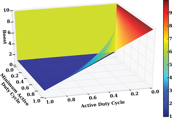
Figure 5. Demonstration of boost as a function of a column’s minimum active duty cycle and active duty cycle.
To study the frequency of boosting, the average number of boosted columns was observed by varying the level of sparseness in the input for both types of inhibition, as shown in Figure 6.11 For the overlap boosting mechanism, equation (20), very little boosting occurs, with boosting occurring more frequently for denser inputs. This is to be expected, as more input columns would be active; thus, causing more competition to occur among the SP’s columns.
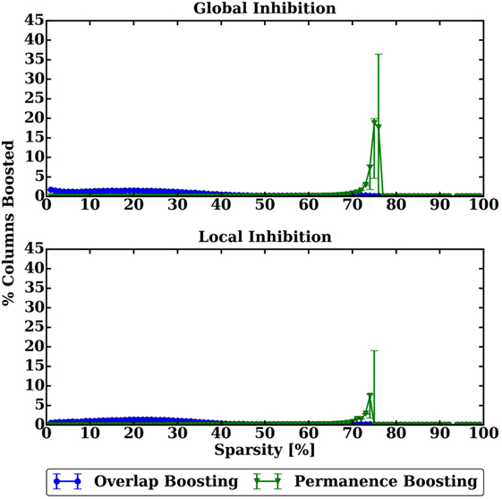
Figure 6. Demonstration of frequency of both boosting mechanisms as a function of the sparseness of the input. The top figure shows the results for global inhibition and the bottom figure shows the results for local inhibition.
For the permanence boosting mechanism, equation (22), boosting primarily occurs when the sparsity is between 70 and 76%, with almost no boosting occurring outside of that range. That boosting is a result of the SP’s parameters. In this experiment, nps = 40 and ρd = 15. Based off those parameters, there must be at least 25 active connected proximal synapses on a column for it have a non-zero overlap; i.e., if the sparsity is 75%, a column would have to be connected to each active column in the input to obtain a non-zero overlap. As such, if the sparsity is greater than 75%, it will not be possible for the SP’s columns to have a non-zero overlap, resulting in no boosting. For lower amounts of sparsity, boosting was not needed, since adequate coverage of the active input columns is obtained.
Recall that the initialization of the SP is performed randomly. Additionally, the positions of active columns for this dataset are random. That randomness combined with a starved level of activity results in a high degree of volatility. This is observed by the extremely large error bars. Some of the SP’s initializations resulted in more favorable circumstances, since the columns were able to connect to the active input columns.
For the SP to adapt to the lack of active input columns, it would have to boost its permanence. This would result in a large amount of initial boosting, until the permanences reached a high enough value. Once the permanences reach that value, boosting will only be required occasionally, to ensure the permanences never fully decay. This behavior is observed in Figure 7, where the permanence boosting frequency was plotted for a sparsity of 74%. The delayed start occurs because the SP has not yet determined which columns will need to be boosted. Once that set is determined, a large amount of boosting occurs. The trend follows a decaying exponential that falls until its minimum level is reached, at which point the overall degree of boosting remains constant. This trend was common among the sparsities that resulted in a noticeable degree of permanence boosting. The right-skewed decaying exponential was also observed in DeSieno (1988) work.
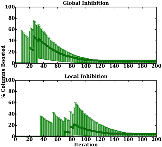
Figure 7. Frequency of boosting for the permanence boosting mechanism for a sparsity of 74%. The top figure shows the results for global inhibition and the bottom figure shows the results for local inhibition. Only the first 200 iterations were shown, for clarity, as the remaining 800 propagated the trend.
These results show that the need for boosting can be eliminated by simply choosing appropriate values for nps and ρd.12 It is thus concluded that these boosting mechanisms are secondary learning mechanisms, with the primary learning occurring from the permanence update in equation (17). These findings allow resource limited systems (especially hardware designs) to exclude boosting, while still obtaining comparable results; thereby, greatly reducing the complexity of the system.
5. Feature Learning
5.1. Feature Selection and Dimensionality Reduction
It is convenient to think of a permanence value as a probability. That probability is used to determine if a synapse is connected or unconnected. It also represents the probability that the synapse’s input is important. It is possible for a given synaptic input to be represented in multiple contexts, where the context for a specific instance is defined to be the set of inputs connected, via proximal synapses, to a column. Due to the initialization of the network, it is apparent that each context represents a random subspace; therefore, each column is learning the probability of importance for its random subset of attributes in the feature space. This is evident in equation (18), as permanences contributing to a column’s activation are positively reinforced and permanences not contributing to a column’s activation are negatively reinforced.
If all contexts for a given synaptic input are observed, the overall importance of that input is obtained. Multiple techniques could be conjured for determining how the contexts are combined. The most generous method is simply to observe the maximum. In this manner, if the attribute was important in at least one of the random subspaces, it would be observed. Using those new probabilities the degree of influence of an attribute may be obtained. Let be defined as the set of learned attribute probabilities, such that represents the probability of Us,a being a meaningful attribute. One form of is shown in equation (26).13 In equation (26), the indicator function is used to mask the permanence values for Us,a. Multiplying that value by every permanence in Φ obtains all of the permanences for Us,a.
Using it is possible to extract a set of meaningful features from the original set of input attributes. This is done by selecting attributes whose corresponding is above some threshold. In the case of equation (26), the threshold is ρs. This is because is representative of the maximum permanence for each attribute in Us, and for a given Us,a to be observed it must be connected, which may only happen when its permanence is at least equal to ρs. The original set of attributes may then be reduced to a new set of meaningful features. This is done by selecting all attributes whose indexes are in , which is obtained by equation (27). Therefore, will contain the set of all indexes in whose . The dimensionality of Us may be reduced to the size of , which will have a length of na or less.
5.2. Input Reconstruction
Building off the feature selection technique, it is possible to obtain the SP’s learned representation of a specific input. To reconstruct the input, the SP’s active columns for that input must be captured. This is naturally done during inhibition, where is constructed. , a function of Us, is used to represent a specific input in the context of the SP.
Determining which permanences caused the activation is as simple as using to mask Φ. Once that representation has been obtained, is used to obtain the overall permanence for the attributes. Those steps will produce a valid probability for each attribute; however, it is likely that there will exist probabilities that are not explicitly in {0, 1}. To account for that, the same technique used for dimensionality reduction is applied, by simply thresholding the probability at ρs. This process is shown in equation (28),14 where is defined to be the reconstructed input.
Thornton and Srbic (2013) used a similar approach for showing how the representation of the input to the SP is understood. The key advantage of this approach is that the input is able to be reconstructed based solely off the permanences and the active columns. This is a novel approach that allows for the input to be decoupled from the system.
6. Experimental Results and Discussion
To empirically investigate the performance of the SP, a Python implementation of the SP was created, called math HTM (mHTM).15 This library was built using the mathematical framework described in this work. An initial implementation of the SP was previously created following the original algorithmic definition. Using the new math-based framework, a speedup of three orders of magnitude was obtained.
The SP was tested on both spatial data as well as categorical data. The details of those experiments are explained in the ensuing subsections.
6.1. Spatial Data
The SP is a spatial algorithm, as such, it should perform well with inherently spatial data. To investigate this, the SP was tested with a well-known computer vision task. The SP requires a binary input; as such, it was desired to work with images that were originally black and white or could be readily made black and white without losing too much information. Another benefit of using this type of image is that the encoder16 may be de-emphasized, allowing for the primary focus to be on the SP. With those constraints, the modified National Institute of Standards and Technology’s (MNIST’s) database of handwritten digits (LeCun et al., 1998) was chosen as the dataset.
The MNIST images are simple 28 × 28 grayscale images, with the bulk of the pixels being black or white. To convert them to black and white images, each pixel was set to “1” if the value was greater than or equal to 255/2 and “0” otherwise. Each image was additionally transformed to be one-dimensional by horizontally stacking the rows. The SP has a large number of parameters, making it difficult to optimize the parameter selection. To help with this, 1,000 independent trials were created, all having a unique set of parameters. The parameters were randomly selected within reasonable limits.17 Additionally, parameters were selected such that . To reduce the computational load, the size of the MNIST dataset was reduced to 800 training inputs and 200 testing inputs. The inputs were chosen from their respective initial sets using a stratified shuffle split with a total of five splits. To ensure repeatability and to allow proper comparisons, care was taken to ensure that both within and across experiments the same random initializations were occurring. After performing the initial experimental batch, the final parameters were selected. Using those parameters, the full MNIST dataset was used. To perform the classification, a linear support vector machine (SVM) was utilized. The input to the SVM was the corresponding output of the SP.
Three comparisons were explored for both global and local inhibition: using the set of active columns as the features (denoted as “column”), using as the features (denoted as “probabilistic”) and using the dimensionality reduced version of the original input as the new input (denoted as “reduction”). The results are shown in Table 2 18 and Table 3 19 for global and local inhibition, respectively. For reference, the same SVM without the SP resulted in an error of 7.95%. The number of dimensions was reduced by 38.01 and 35.71% for global and local inhibition, respectively. Both the probabilistic and reduction methods only performed marginally worse than the base SVM classifier. Considering that these two techniques are used to modify the raw input, it is likely that the learned features were the face of the numbers (referring to attributes equaling “1”). In that case, those methods would almost act as pass through filters, as the SVM is already capable of determining which attributes are more/less significant. That being said, being able to reduce the number of attributes by over two thirds, for the local inhibition case, while still performing relatively close to the case where all attributes are used is quite desirable.
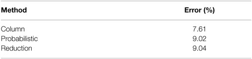
Table 2. SP performance on MNIST using global inhibition.
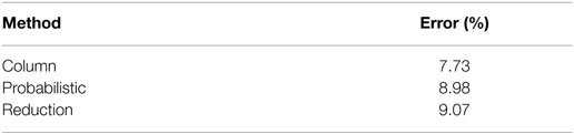
Table 3. SP performance on MNIST using local inhibition.
Using the active columns as the learned feature is the default behavior, and it is those activations that would become the feedforward input to the next level (assuming an HTM with multiple SPs and/or TMs). Both global and local inhibition outperformed the SVM, but only by a slight amount. Considering that only one SP region was utilized, that the SP’s primary goal is to map the input into a new domain to be understood by the TM, and that the SP did not hurt the SVM’s ability to classify, the SP’s overall performance is acceptable. It is also possible that given a two-dimensional topology and restricting the initialization of synapses to a localized radius may improve the accuracy of the network. Comparing global to local inhibition, comparable results are obtained. This is likely due to the globalized formation of synaptic connections upon initialization, since that results in a loss of the initial network topology.
To explore the input reconstruction technique, a random instance of each class from MNIST was selected. The input was then reconstructed as shown in Figure 8.20 The top row shows the original representation of the inputs. The middle row shows the SDR of the inputs. The bottom row shows the reconstructed versions. The representations are by no means perfect, but it is evident that the SP is indeed learning an accurate representation of the input.
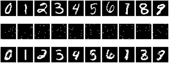
Figure 8. Reconstruction of the input from the context of the SP. Shown are the original input images (top), the SDRs (middle), and the reconstructed version (bottom).
6.2. Categorical Data
One of the main purposes of the SP is to create a spatial representation of its input through the process of mapping its input to SDRs. To explore this, the SP was tested on Bohanec and Rajkovic (1988) and Lichman (2013) car evaluation dataset. This dataset consists of four classes and six attributes. Each attribute has a finite number of states with no missing values. To encode the attributes, a multivariate encoder comprised of categorical encoders was used.21 The class labels were also encoded, by using a single category encoder.22
The selection of the SP’s parameters was determined through manual experimentation.23 Cross validation was used, by partitioning the data using a stratified shuffle split with eight splits. To perform the classification an SVM was utilized, where the output of the SP was the corresponding input to the SVM. The SP’s performance was also compared to just using the linear SVM and using a random forest classifier.24 For those classifiers, a simple preprocessing step was performed to map the text-based values to integers.
The results are shown in Table 4.25 The SVM performed poorly, having an error of 26.01%. Not surprisingly, the random forest classifier performed much better, obtaining an error of 8.96%. The SP was able to far outperform either classifier, obtaining an error of only 2.32%. From literature, the best known error on this dataset was 0.37%, which was obtained from a boosted multilayer perceptron (Oza, 2005).
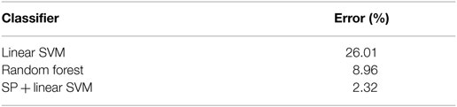
Table 4. Comparison of classifiers on car evaluation dataset.
This result shows that the SP was able to map the input data into a suitable format for the SVM, thereby drastically improving the SVM’s classification. Based off this, it is determined that the SP produced a suitable encoding.
6.3. Extended Discussion
Comparing the SP’s performance on spatial data to that of categorical data provides some interesting insights. It was observed that on spatial data the SP effectively acted as a pass through filter. This behavior occurs because the data is inherently spatial. The SP maps the spatial data to a new spatial representation. This mapping allows classifiers, such as an SVM, to be able to classify the data with equal effectiveness.
Preprocessing the categorical data with the SP provided the SVM with a new spatial representation. That spatial representation was understood by the SVM as readily as if it were inherently spatial. This implies that the SP may be used to create a spatial representation from non-spatial data. This would thereby provide other algorithms, such as the TM and traditional spatial classifiers, a means to interpret non-spatial data.
7. Exploring the Primary Learning Mechanism
To complete the mathematical formulation, it is necessary to define a function governing the primary learning process. Within the SP, there are many learned components: the set of active columns, the neighborhood (through the inhibition radius), and both of the boosting mechanisms. All of those components are a function of the permanence, which serves as the probability of an input column being active in various contexts.
Let be defined as the permanence update amount, as shown in equation (29), where . δΦ may then be rewritten as . Similarly, the permanence update for is given by , where .
The permanence update equation is then logically split into two distinct components. The first component is the set of active columns, which is used to determine the set of permanences to update. The second component is ΔΦ, which is used to determine the permanence update amount.
7.1. Plausible Origin for the Permanence Update Amount
It is noticed that ΔΦ represents an unlearned function of a random variable coming from a prior distribution. That random variable is nothing more than X. It is required that , where Ber is used to denote the Bernoulli distribution. Recall that the initialization of the SP is performed such that each Xi,k ∈ Xi is obtained by randomly sampling without replacement from Us. Each Xi ∈ X is independent, since they are obtained by sampling from the same Us. This initialization scheme means that each Xi ∈ X is independent and identically distributed (i.i.d.), but that each Xi,k ∈ Xi is not i.i.d.
If the initialization scheme is redefined such that Xi,k ∈ Xi is obtained by sampling with replacement, then each Xi,k ∈ X would be i.i.d. This slight change to the initialization would mean that a given input attribute may be observed by a column zero up to nps times. If nc is set to be sufficiently large, then each Us,a will still be observed and the overall impact of this change should be minor. Assuming that this new initialization scheme is utilized, then Ber(θ), where θ is defined to be the probability of an input being active. Using the PMF of the Bernoulli distribution, the likelihood of θ given X is obtained in equation (30), where t ≡ ncnps and , the overall mean of X. The corresponding log-likelihood of θ given X is given in equation (31).
Taking the gradient of the log-likelihood of equation (31) with respect to θ results in equation (32). Similarly, the partial derivative of the log-likelihood for a single Xi,k results in equation (33). Equation (33) suggests by its form that an unconstrained local update of θ may be obtained. Let ), such that Θi,k = ℙ(Ai,k). Recall that X is populated based off the entries in a single Us, i.e., X represents the current input to the SP, not all of the inputs. Solving equation (32) for the maximum-likelihood estimator results in maximizing the likelihood of the current sample rather than the population. Realizing this, an approach similar to stochastic gradient ascent is used to obtain equation (34), where and are functions of that compute the permanence increment and decrement amount for each , respectively.
Relating equation (34) to equation (29), and were defined to return the constants ϕ+ and ϕ−, respectively. If the probabilities of each Xi,k = 1 are sufficiently close in value for all Us ∈ U, then global constants may be sufficient. Using constants also simplifies the permanence update equation, which is likely why the original permanence update method, equation (18), used this approach. For more complicated inputs, it is unlikely that this assumption will hold true. To address that, this new method allows for a local and adaptive way to tune the permanences.
7.2. Discussing the Permanence Selection
The set of active columns is the learned component in equation (18). Those columns are used to determine which permanences are selected for update. Obtaining the set of active columns is done through a process similar to competitive learning (Rumelhart and Zipser, 1985). In a competitive learning network, each neuron in the competitive learning layer is fully connected to each input neuron. The neurons in the competitive layer then compete, with one neuron winning the competition. The neuron that wins sets its output to “1” while all other neurons set their output to “0”. At a global scale, this resembles the SP with two key differences. The SP permits multiple columns to be active at a time and each column is connected to a different subset of the input’s attributes.
Posit that each column is equivalent to a competitive learning network. This would create a network with one neuron in the competitive layer and nps neurons in the input layer. The neuron in the competitive layer may only have the state of “1” or “0”; therefore, only one neuron would be active at a time. Given this context, each column is shown to follow the competitive learning rule.
Taking into context the full SP, with each column as a competitive learning network, the SP could be defined to be a bag of competitive learning networks, i.e., an ensemble with a type of competitive learning network as its base learner. Recalling that X ⊆ Us, each Xi is an input for . Additionally, each Xi is obtained by randomly sampling Us without replacement. Comparing this ensemble to attribute bagging (Bryll et al., 2003), the primary difference is that sampling is done without replacement instead of with replacement.
In attribute bagging, a scheme, such as voting, must be used to determine what the result of the ensemble should be. For the SP, a form of voting is performed through the construction of . Each base learner (column) computes its degree of influence. The max degree of influence is nps. Since that value is a constant, each may be represented as a probability by simply dividing by q. In this context, each column is trying to maximize its probability of being selected. During the inhibition phase, a column is chosen to be active if its probability is at least equal to the ρc-th largest probability in its neighborhood. This process may then be viewed as a form of voting, as all columns within a neighborhood cast their overlap value as their vote. If the column being evaluated has enough votes, it will be placed in the active state.
8. Conclusion and Future Work
In this work, a mathematical framework for HTM’s SP was presented. Using the framework, it was demonstrated how the SP can be used for feature learning. The primary learning mechanism of the SP was explored. It was shown that the mechanism consists of two distinct components, permanence selection and the degree of permanence update. A plausible estimator was provided for determining the degree of permanence update, and insight was given on the behavior of the permanence selection.
The findings in this work provide a basis for intelligently initializing the SP. Due to the mathematical framework, the provided equations could be used to optimize hardware designs. Such optimizations may include removing the boosting mechanism, limiting support to global inhibition, exploiting the matrix operations to improve performance, reducing power through the reduction of multiplexers, etc… In the future, it is planned to explore optimized hardware designs. Additionally, it is planned to make the SP more flexible and adaptive. Finally, it is planned to expand this work to provide the same level of understanding for the TM.
Author Contributions
JM wrote the paper, formulated the initial mathematics, developed mHTM, and conducted the experiments. EF assisted in the formalization of the mathematics. DK initiated the work and assisted in experimental design. All listed authors made substantial intellectual contributions to the work and approve it for publication.
Conflict of Interest Statement
The authors declare that the research was conducted in the absence of any commercial or financial relationships that could be construed as a potential conflict of interest.
Acknowledgments
The authors would like to thank Kevin Gomez of Seagate Technology, the staff at RIT’s research computing, and the members of the NanoComputing Research Lab, in particular Amanda Hartung and Cory Merkel, for their support and critical feedback. The authors would also like to thank the reviewers for their exhaustive feedback to enhance the overall quality of the paper.
Footnotes
- ^This parameter was originally referred to as the minimum overlap; however, it is renamed in this work to allow consistency between the SP and the TM.
- ^All indices start at 0.
- ^The parameters and have default values of 0.01 and 0.1, respectively.
- ^ was used as a probability. Because , permanences are uniformly initialized with a mean of , and for a proximal synapse to be connected it must have a permanence value at least equal to , may be used to represent the probability that an initialized proximal synapse is connected.
- ^Due to X being binary, a bitwise negation is equivalent to the shown logical negation. In a similar manner, the multiplications of with X and ¬X can be replaced by an AND operation (logical or bitwise).
- ^The conditions within the piecewise function must be evaluated top-down, such that the first condition takes precedence over the second condition which takes precedence over the third condition.
- ^The distance function is typically the Euclidean distance.
- ^In an actual system the positions would be explicitly defined.
- ^It is assumed that an SP column and an input column do not coincide, i.e., their distance is greater than zero. If this occurs, D will be unstable, as zeros will refer to both valid and invalid distances. This instability is accounted for during the computation of the inhibition radius, such that it will not impact the actual algorithm.
- ^The summation of the connected synapses is lower bounded by one to avoid division by zero.
- ^To obtain Figure 6, the average number of boosted columns during each epoch is computed. The average, across all of those epochs, is then calculated. That average represents the percentage of columns boosted for a particular level of sparsity. It is important to note that because the SP’s synaptic connections are randomly determined, the only dataset specific factors that will affect how the SP performs will be na and the number of active input columns. This means that it is possible to generalize the SP’s behavior for any dataset, provided that the dataset has a relatively constant number of active columns for each input. For the purposes of this experiment, the number of active input columns was kept fixed, but the positions were varied; thereby creating a generalizable template. The inputs presented to the SP consisted of 100 randomly vectors with a width of 100 columns. Within each input, the columns were randomly set to be active. The sparseness is then the percentage of non-active input columns. Each simulation consisted of 10 epochs and was performed across 10 trials. The SP’s parameters are as follows: nc = 2048, na = 100, nps = 40, ρd = 15, ρs = 0.5, ϕδ = 0.05, = , ϕ+ = 0.03, ϕ− = 0.05, β0 = 10, and τ = 100. Synapses were trimmed if their permanence value ever reached or fell below 10−4. On the figure, each point represents a partial box plot, i.e., the data point is the median, the upper error bar is the third quartile, and the lower error bar is the first quartile.
- ^This assumes that there will be enough active columns in the input. If this is not the case, the input may be transformed to have an appropriate number of active columns.
- ^The function max was used as an example. Other functions producing a valid probability are also valid.
- ^The function max was used as an example. If a different function is utilized, it must be ensured that a valid probability is produced. If a sum is used, it could be normalized; however, if caution is not applied, thresholding with respect to may be invalid and therefore require a new thresholding technique.
- ^This implementation has been released under the MIT license and is available at: https://github.com/tehtechguy/mHTM.
- ^An encoder for HTM is any system that takes an arbitrary input and maps it to a new domain (whether by lossy or lossless means) where all values are mapped to the set 0, 1.
- ^The following parameters were kept constant: = 0.5, 30 training epochs, and synapses were trimmed if their permanence value ever reached or fell below .
- ^The following parameters were used to obtain these results: nc = 936, nps = 353, ρd = 14, ϕδ = 0.0105, ρc = 182, ϕ+ = 0.0355, ϕ− = 0.0024, β0 = 18, and τ = 164.
- ^The following parameters were used to obtain these results: nc = 786, nps = 267, ρd = 10, ϕδ = 0.0425, ρc = 57, ϕ+ = 0.0593, ϕ− = 0.0038, β0 = 19, and τ = 755.
- ^The following parameters were used to obtain these results: nc = 784, nps = 392, ρd = 10, ϕδ = 0.01, ρc = 10, ϕ+ = 0.001, ϕ− = 0.002, ten training epochs, global inhibition, and boosting was disabled. The number of columns was set to be equal to the number of attributes to allow for a 1:1 reconstruction of the SDRs.
- ^A multivariate encoder is one which combines one or more other encoders. The multivariate encoder’s output concatenates the output of each of the other encoders to form one SDR. A categorical encoder is one which losslessly converts an item to a unique SDR. To perform this conversion, the number of categories must be finite. For this experiment, each category encoder was set to produce an SDR with a total of 50 bits. The number of categories, for each encoder, was dynamically determined. This value was set to the number of unique instances for each attribute/class. No active bits were allowed to overlap across encodings. The number of active bits, for each encoding, was scaled to be the largest possible value. That scaling would result in utilizing as many of the 50 bits as possible, across all encodings. All encodings have the same number of active bits. In the event that the product of the number of categories and the number of active bits is less than the number of bits, the output was right padded with zeros.
- ^This encoding followed the same process as the category encoders used for the attributes.
- ^The following parameters were used: nc = 4096, nps = 25, ρd = 0, ϕδ = 0.5, ρc = 819, ϕ+ = 0.001, and ϕ− = 0.001. Boosting was disabled and global inhibition was used. Only a single training epoch was utilized. It was found that additional epochs were not required and could result in overfitting. was intentionally set to be about 20% of . This deviates from the standard value of ∼2%. A value of 2% resulted in lower accuracies (across many different parameter settings) than 20%. This result is most likely a result of the chosen classifier. For use with the TM or a different classifier, additional experimentation will be required.
- ^These classifiers were utilized from scikit-learn (2016).
- ^The shown error is the median across all splits of the data.
References
Ahmad, S., and Hawkins, J. (2015). Properties of sparse distributed representations and their application to hierarchical temporal memory. arXiv preprint arXiv:1503.07469. Available at: https://arxiv.org/abs/1503.07469
Bohanec, M., and Rajkovic, V. (1988). “Knowledge acquisition and explanation for multi-attribute decision making,” in 8th Intl Workshop on Expert Systems and Their Applications, (Avignon) 59–78.
Bryll, R., Gutierrez-Osuna, R., and Quek, F. (2003). Attribute bagging: improving accuracy of classifier ensembles by using random feature subsets. Pattern Recognit. 36, 1291–1302. doi: 10.1016/S0031-3203(02)00121-8
Byrne, F. (2015). Encoding reality: prediction-assisted cortical learning algorithm in hierarchical temporal memory. arXiv preprint arXiv:1509.08255. Available at: https://arxiv.org/abs/1509.08255
Cui, Y., Ahmad, S., and Hawkins, J. (2016). Continuous online sequence learning with an unsupervised neural network model. Neural Comput. 28, 2474–2504. doi:10.1162/NECO_a_00893
DeSieno, D. (1988). “Adding a conscience to competitive learning,” in IEEE International Conference on Neural Networks, 1988 (San Diego, CA: IEEE), 117–124.
Gersho, A., and Gray, R. M. (2012). Vector Quantization and Signal Compression, Vol. 159. New York: Springer Science & Business Media.
Hawkins, J., and Ahmad, S. (2016). Why neurons have thousands of synapses, a theory of sequence memory in neocortex. Front. Neural Circuits 10:1–13. doi:10.3389/fncir.2016.00023
Hawkins, J., Ahmad, S., and Dubinsky, D. (2011). Hierarchical Temporal Memory Including htm Cortical Learning Algorithms. Available at: http://numenta.org/resources/HTM_CorticalLearningAlgorithms.pdf
Hawkins, J., and George, D. (2007). Directed Behavior using a Hierarchical Temporal Memory Based System. Google Patents. Available at: https://www.google.com/patents/US20070192268. US Patent App. 11/622,448.
Hebb, D. O. (1949). The Organization of Behavior: A Neuropsychological Approach. New York: John Wiley & Sons.
Kohonen, T. (1982). Self-organized formation of topologically correct feature maps. Biol. Cybern. 43, 59–69. doi:10.1007/BF00337288
Lattner, S. (2014). Hierarchical Temporal Memory-Investigations, Ideas, and Experiments. Master’s thesis, Linz: Johannes Kepler Universität.
Lavin, A., and Ahmad, S. (2015). “Evaluating real-time anomaly detection algorithms–the numenta anomaly benchmark,” in IEEE 14th International Conference on Machine Learning and Applications (ICMLA) (Miami: IEEE), 38–44.
Leake, M., Xia, L., Rocki, K., and Imaino, W. (2015). A probabilistic view of the spatial pooler in hierarchical temporal memory. World Acad. Sci. Eng. Technol. Int. J. Comput. Electr. Autom. Control Inform. Eng. 9, 1111–1118.
LeCun, Y., Bottou, L., Bengio, Y., and Haffner, P. (1998). Gradient-based learning applied to document recognition. Proc. IEEE 86, 2278–2324. doi:10.1109/5.726791
Lichman, M. (2013). UCI Machine Learning Repository. Available at: http://archive.ics.uci.edu/ml
Numenta. (2016). Numenta Platform for Intelligent Computing (Nupic). Available at: http://numenta.org/
Oza, N. C. (2005). “Online bagging and boosting,” in IEEE International Conference on Systems, Man and Cybernetics, Vol. 3 (Waikoloa: IEEE), 2340–2345.
Rumelhart, D. E., and Zipser, D. (1985). Feature discovery by competitive learning. Cogn. Sci. 9, 75–112. doi:10.1207/s15516709cog0901_5
scikit-learn. (2016). scikit-learn. Available at: http://scikit-learn.org/stable/index.html
Keywords: hierarchical temporal memory, spatial pooler, machine learning, neural networks, self-organizing feature maps, unsupervised learning
Citation: Mnatzaganian J, Fokoué E and Kudithipudi D (2017) A Mathematical Formalization of Hierarchical Temporal Memory’s Spatial Pooler. Front. Robot. AI 3:81. doi: 10.3389/frobt.2016.00081
Received: 08 September 2016; Accepted: 26 December 2016;
Published: 30 January 2017
Edited by:
Christof Teuscher, Portland State University, USAReviewed by:
Ashley Prater, United States Air Force Research Laboratory, USASubutai Ahmad, Numenta Inc., USA
Copyright: © 2017 Mnatzaganian, Fokoué and Kudithipudi. This is an open-access article distributed under the terms of the Creative Commons Attribution License (CC BY). The use, distribution or reproduction in other forums is permitted, provided the original author(s) or licensor are credited and that the original publication in this journal is cited, in accordance with accepted academic practice. No use, distribution or reproduction is permitted which does not comply with these terms.
*Correspondence: James Mnatzaganian, jamesmnatzaganian@outlook.com