Analysis of Worldwide Time-Series Data Reveals Some Universal Patterns of Evolution of the SARS-CoV-2 Pandemic

1 Introduction

In cooperative social dynamics [1, 2], the genesis of a collective phenomenon arising from contagious social interactions involves mechanisms of self-organised criticality [3, 4]. It depends on each individual involved, based on its actual contacts, psychology and behaviour. In the presence of viruses, these mechanisms are additionally shaped by firm biological factors. Recent developments of SARS-CoV-2 pandemic [5, 6] revealed a specific global phenomenon emerging from the stochastic multi-scale processes. The infection incidence occurs with a high temporal resolution at the interactions between the virus and human hosts, whose biological features, social behaviours and mobility [7] significantly contribute to the epidemic’s spreading [8]. At the molecular scale, the virus-host interactions [9–11] crucially depend on the virus biology and genetic factors determining the host’s immunity towards the virus in question [12, 13]. Thus, the occurrence of an infection event and the infection manifestation may lead to a range of different scenarios from asymptomatically infected to severe health issues and fatalities [14–17]. Multiple other factors may play a role [18], depending on the population genetic features and social life [19]. They include cultural, political and economic aspects, official and spontaneous reaction to the crisis, and the organisation of the health care system, all of which may significantly differ between different geographical locations [20]. Moreover, the actual impact of these factors changes over time as the epidemic develops, in particular, since the appropriate vaccines targeting SARS-CoV-2 viruses [3, 21] are available, thus enabling potentially substantial changes due to massive immunisation of the population given the theoretical analysis in [22–24]. Attempts were made to identify different parameters that may influence the epidemic and estimate their mutual interdependence and impact. For example, the human-development index, built-up-area-per-capita, and the immunisation coverage appear among the statistically high-ranking drivers of SARS-CoV-2 epidemic [18].

In addition, temporal variations occur at all scales, from the virus mutations [11] to changed behaviours of each individual and population groups, e.g., due to the government imposed measures [6, 25], or adaptation caused by the awareness of the current epidemiological situation [26, 27]. These variations increase the stochasticity of the infection and contact processes, making the prediction of their output even more difficult. For real-time epidemic management and the predictions of further developments, it is crucial to understand the nature of the underlying stochastic processes and the factors that can significantly influence them. For this purpose, the empirical data analysis and theoretical modelling [28] provide complementary views of these complex processes. For example, agent-based models capture the interplay of the bio-social factors at the elementary scale of the virus-host interactions at high temporal resolution [8, 29–37]. On the other hand, more traditional compartmental models [38] consider a coarse-grained picture of the population groups having different roles in the process. Another research line aims at the mathematical description of the exact empirical data, in particular, for the outbreak phase [39, 40]. For instance, different studies provided tangible arguments for the cause of the changing shape of the infection curve comprising the appearance of linear and power-law segments [41, 42], prolonged stagnation periods, and multiple waves [43]. Since the beginning of the epidemic, empirical data were collected over different countries or provinces [44]. Despite the coarse-grained spatial and temporal structure (daily resolution), these data may contain relevant information about the temporal aspects of the epidemic at different geographical locations. Previous studies, based on the empirical data regarding the dynamics of interacting units in many complex systems, provided valuable information about the related stochastic processes. Some striking examples across different spatial and temporal scales include the influence of the world financial index dynamics on different countries [45, 46], traffic jamming [47, 48], brain-to-brain coordination dynamics [49, 50], and the cooperative gene expressions along different phases of the cell cycle [51, 52]. Similarly, the collected data of SARS-CoV-2 spreading enable a possibility to investigate the infection dynamics in various details and more appropriate modelling of the emergent behaviours. In this respect, a larger-scale picture may emerge by studying temporal fluctuations of the world infection dynamics. More subtle questions regard the indicators for hidden mechanisms arising from the interplay of the above-mentioned biological factors and different social behaviours [8, 27, 29, 53, 54] behind the observed epidemic development.

In this work, we address some of these critical issues aiming to unveil the inherent features of infection dynamics by studying time-series data that are publicly available at GitHub [44] collected over different countries or regions (provinces). Using the datasets of the daily recorded number of confirmed infection cases, we consider two separate segments of time series. Defining two distinct 8-month periods in the epidemic’s evolution is motivated by the appearance of SARS-CoV-2 vaccines in the latter period, enabling pharmaceutical intervention measures not available in the outbreak phase, cf. Figure 1. Namely, the records for the first 8 months of the epidemic, starting from the first registered case in each country, represent the epidemic’s outbreak phase. Meanwhile, the last 8 months (preceding the data collection on 30 September 2021), during which the pharmaceutical intervention was available in most of the countries, characterises the initial immunisation phase of this pandemic. Our quantitative analysis comprises three levels of information: the network mapping and spectral analysis, K-means clustering of pairs of time series, and detrended fractal analysis of individual time series. Each of these methods provides just partial information about the studied dynamics. We combine them to create a comprehensive picture of the course of the epidemic in different countries and how they relate to each other. In addition to quantifying the differences between the outbreak and immunisation phase, our results reveal two global features of the SARS-CoV-2 pandemic. Firstly, the worldwide groups of countries (and provinces) robustly appear in clusters having a similar temporal evolution of the infection dynamics. This clustering suggests that the environmental and socio-economical factors and government-imposed measures can certainly influence small-scale fluctuation characteristics of the clusters but do not significantly change the course of the process on larger scales. Secondly, the epidemic evolution exhibits ubiquitous waves driven by the cyclic infection dynamics, where several typical cycles appear associated with the identified clusters. Again, the shape of these specific cycles coincides with the mentioned clustering mechanisms. Hence, their origin and potential control will remain challenging within purely social measures. A more detailed analysis of the complex feedback between biological and social factors at all scales is needed.

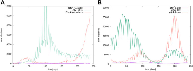
FIGURE 1. Examples of time series. Temporal evolution of confirmed infection cases in different countries, belonging to different groups in the outbreak (A) and immunisation phase (B).

2 Materials and Methods

2.1 Data Acquisition, Preparation, and Mapping

We consider the worldwide data of the number of new infection cases downloaded from GitHub [44]. The dataset contains the number of daily detected new cases for 279 countries including separated data for some provinces. For this work, we select time series in two eight-mount periods comprising the epidemic’s outbreak phase (starting from the first registered case in a given country or province) and the immunisation phase (22 January 2020 until 30 September 2021). The corresponding number of countries and provinces with the active epidemic’s data traced in both periods is 255. For instance, the first case in France was detected on 24 January 2020, and thus the outbreak time series covers the period from that date until 19 September 2020. However, Slovenia had the first registered case on 5 March 2020; hence its outbreak time series cover 5 March until 30 October 2020. Meanwhile, the immunisation period is from 3 February 2021 to 30 September 2021, equal for all considered countries and provinces.

By mapping these datasets, we obtain two correlation networks for the outbreak and immunisation phase, respectively, where the network’s links stand for significant positive correlations. We first compute the Pearson’s correlation coefficient for the corresponding pairs (i, j) of the time series

where τ ∈ {O, V}, ${\mu }_i^{\tau }$ is average value of the time series of country i during period τ, ${\sigma }_i^{\tau }$ is standard deviation of time series $X_i^{\tau }(t)$, and N_T = 240 is the length of time series. To remove spurious correlations, we apply the filtering procedure standardly used in these type of network mapping [47, 49, 51]. More precisely, the matrix elements $C_{ij}^{\tau }$ are first transformed to the interval [0, one] by $C{P}_{ij}^{\tau }=\frac{1}{2}(C_{ij}^{\tau }+1)$, and then multiplied by a factor $M_{ij}^{\tau }$ which is obtained in the following way. From the rows i and j, the diagonal elements are removed and the considered elements $C{P}_{ij}^{\tau }$ and $C{P}_{ji}^{\tau }$ are placed at the beginning of the row i and j, respectively, thus obtaining two n = N − 1 dimensional vectors $\widetilde{C{P}_i^{\tau }}$ and $\widetilde{C{P}_j^{\tau }}$. Then $M_{ij}^{\tau }$ is computed as Pearson’s coefficient between these two vectors. The matrix element of the filtered correlation matrix $\overline{C_{ij}^{\tau }}=M_{ij}^{\tau }C{P}_{ij}^{\tau }$ is then mapped back to the interval [ − 1, 1]. Finally, the elements of the network’s adjacency matrix are defined as $A_{ij}^{\tau }=1$ when the matrix elements $\overline{C_{ij}^{\tau }}>\theta$ exceed a specified threshold value θ, and zero otherwise. The threshold value θ is determined concerning the network’s spectral properties, as described below.

2.2 Network’s Spectral Analysis and Community Detection

The above-described data mapping should lead to undirected unweighted networks; the nodes represent countries (or provinces), and links indicate the positive correlations between infection incidences exceeding a threshold θ. We use the spectral properties of networks to obtain the adequate threshold value, where the guiding criteriums are the network’s sparseness and the relative stability of the community structure. Starting from θ = 0, we increase it by the value 0.05 and solve the eigenvalue problem of the corresponding adjacency matrix, Av_i = λ_iv_i|_θ, and calculate the spectrum ${\{{\lambda }_1,\dots ,{\lambda }_N\}}_{\theta }$ for each threshold θ. We compare the adjacency matrix spectrum for network θ = 0 with spectra of each network obtained for considered θ > 0 using Kolmogorov-Smirnov (KS) distance. For each θ > 0 we obtain one KS distance and plot its dependence of θ, see Figure 2B. The KS-distance has a minimum of around θ = 0.5 for the outbreak and immunisation phase. We use this value of θ to obtain the networks used in our analysis.

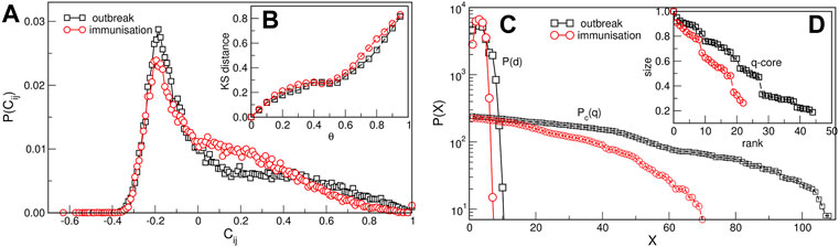
FIGURE 2. Network measures. (A) The normalised probability density function of the filtered correlation coefficients for the outbreak and immunisation periods. (B) The Kolmogorov-Smirnov distance between the eigenvalue spectrums of networks obtained for θ = 0 and different values of θ > 0, plotted against θ > 0. (C) The distribution of the shortest-path distances P(d) vs. the distance d and the cumulative distribution P_c(q) of the node’s degree q for the outbreak and immunisation networks with the threshold θ = 0.5. (D) The size of the q-core of these networks plotted against the q-rank.

We study the community structure of the networks for the outbreak and immunisation period using spectral analysis and the eigenvalue problem of the normalised Laplacian related to the network’s adjacency matrix. In mathematics theory [55, 56], the number of smallest non-zero eigenvalues of the Laplacian matrix is a good indicator of the number of communities. The matrix elements of the normalised Laplacian for undirected binary network represented by the adjacency matrix A are defined as

where q_i and q_j are degrees of nodes i and j. For the normalised Laplacian [2], we solve the eigenvalue equation $\mathbf{L}{v}^L={\lambda }_i^N{v}_i^L$ and determine all eigenvalues and eigenvectors. In the case of a connected network, these eigenvalues are non-negative. One zero-eigenvalue appears with strictly positive eigenvector’s components [55]. Consequently, the orthogonal eigenvectors corresponding to the three smallest non-zero eigenvalues localise on the communities of the network. Hence, the scatter plot of the components of these eigenvectors shows a branching structure. Each branch contains indexes of the non-zero eigenvector components, that is, the nodes belonging to a network’s community [56].The size of the q-core of the networks is determined by removing the nodes with the increasing degree q. Several other graph properties are determined, and the networks are visualised using Gephi software [57].

2.3 K-Means Clustering of Time Series

The implementation of the K-means algorithm for clustering of time series in Python known as tslearn [58] is used. K-means is an unsupervised machine learning algorithm that aggregates data points according to similarities, starting with K randomly positioned centroids. Based on these centroids, data points are assigned to the centroid closest to that data point according to some distance metric. The algorithm consists of a certain number of iterative (repetitive) calculations used to optimise the positions of the centroids. Considering each time series of length N_T as a data point in N_T dimensional space, the appropriate measures enable calculating the distances between these data points. We use the Dynamic Time Wrapping (DTW) algorithm to align time series with centroids and measure their similarities. The DTW is a widely used algorithm measuring similarities between time series and their classification. It does not transform the time series; it only finds the minimal distance between time series beyond simple correlation. Specifically, it performs an optimal alignment between two time series by matching the indices from the first time series to the second time series, subject to several constraints. The mapping of indices from the first series to the second series must be monotonically increasing. For the indices i > j from the first time series, there must be two indices from the second series l > k such that i is matched with l and j is matched with k. Meanwhile, the first index from the first series must match the first index of the second time series, and similarly, the last index from the first series must be matched to the last index of the second time series, but these points may have more other matches. The optimal alignment is the one that satisfies all of these restrictions with the minimal cost, where cost is the sum of absolute differences of values for each matched pair of indices. The DTW distance in the K-means algorithm is the value of cost. We use the K-means algorithm with DTW distance to cluster time series and find centroids. Each centroid is again a time series that describes the average behaviour of the time series belonging to one cluster.

2.4 Trends and Fractal Analysis of Time Series

Temporal fluctuations are studied by the fractal detrended analysis of each time series. For each time series x(k), k = 1, 2, ⋯T, the profile $Y(i)={\sum }_{k=1}^i(x(k)-<x>)$ of the time series is divided in N_s segments of the length n. The fluctuation function F_q(n) with the varied segment length n is defined as

Here, $F^2(\mu ,n)=\frac{1}{n}{\sum }_{i=1}^n{\left[Y((\mu -1)n+i)-y_{\mu }(i)\right]}^2$ is the standard deviation from a local trend y_μ(i) on the segment μ. For q = 2, we determine the Hurst exponent h₂ from the straight-line segments of the log-log plot of the fluctuation function F₂(n). For the multifractal analysis, the values of q ∈ [ − 4, 4] are varied.

To determine cyclic trends, we use the local adaptive detrending algorithm, see [59, 60], where time series is divided into segments of the length 2m + 1 overlapping over m + 1 points. The polynomial interpolation is applied in each segment, and its contribution in the overlapped region is weighted such that it decreases linearly with the distance from the segment’s centre. As stated in the Introduction, we consider worldwide recorded time series of the infection cases. For illustration, a few examples of time series recorded in different countries are shown in Figure 1.

2.5 The Correlation Networks Mapping in the Outbreak and Immunisation Phase

The network mapping is based on the cross-correlation coefficient C_ij of the pairs of time series {i, j} and a suitably selected threshold. Hence, the correlations exceeding the threshold θ are accepted, making the adjacency-matrix elements A_ij(θ) = Θ(C_ij − θ) − δ_ij of an undirected unweighted network. Before selecting the threshold, a filtering procedure was applied to the complete correlation matrix to enhance the positive correlations of interest in this work (see Methods). The applied methodology was proved useful in quantifying correlations of time series in diverse type of data [45, 47–52]. Figure 2A shows probability distributions of filtered correlations coefficients for the outbreak and immunisation period. While both probability distributions have a peak at a value C_ij < 0, they have slightly different shapes. They both have a pronounced tail for positive values of correlation coefficients, where the distribution P(C_ij) for the outbreak period has a slower decay at correlations C_ij > 0.2. The appropriate threshold is selected considering changes in spectral properties of the adjacency matrix with the increasing threshold, as explained in the following. Figure 2B shows the Kolmogorov-Smirnov (KS) distance between the eigenvalues of the A_ij(θ) compared to the one at θ = 0 depending on the threshold θ for the outbreak and immunisation networks. We see that the KS distance grows slowly with θ up to the value $\sim 0.4$; meanwhile, the growth becomes rapid for the values of θ > 0.5 for both networks, suggesting a profound change in the networks’ structure when the threshold exceeds θ = 0.5. Thus, we select this turning point as the optimal threshold value. Moreover, the networks obtained by applying the threshold weight θ = 0.5 are sufficiently sparse; meanwhile, their spectral properties do not differ drastically from the corresponding outbreak and immunisation period networks at θ = 0 containing all positive correlations. The resulting networks for θ = 0.5 are visualised in Figure 3. See also Supplementary Information (SI) for more details.

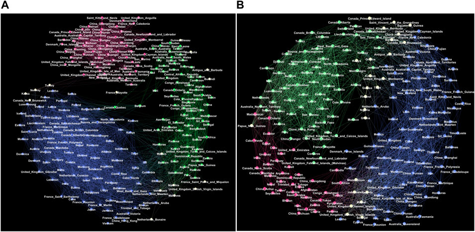
FIGURE 3. Giant connected components of the correlation networks at the threshold θ =0.5 for the outbreak period (A) and the immunisation period (B). Red, green and blue colours indicate groups of nodes in three respective communities G1, G2, G3 in the outbreak network, and g1, g2, g3 in the immunisation period network, determined by the eigenvector-localisation, see text and Figure 4. Unclassified borderline nodes are shown in white colour. Labels on nodes identify the corresponding country or province. The complete lists of nodes in each community are given in Supplementary Tables S1–S6 in Supplementary Information.

The giant connected component of each network exhibits a community structure, i.e., the occurrence of groups of nodes that are better connected among themselves than with the nodes outside that group, cf. Figure 3. The identity of nodes comprising each community is determined using the localisation of the eigenvectors associated with the three lowest nonzero eigenvalues of the normalised Laplacian operator [55], as explained in Methods [56]. The eigenvalues of the normalised Laplacians for two networks are shown in ranking order in Figure 4, middle panel. Several lowest nonzero eigenvalues appear to be separated from the bulk in both networks. This network feature is compatible with the existence of mesoscale communities, on which the corresponding eigenvectors tend to localise [55, 56]. The scatterplots of the eigenvectors associated with three lowest nonzero eigenvalues, see Figure 4, show three differentiable branches, here indicated as G1, G2, G3 for the outbreak, and g1, g2, g3 for the immunisation phase network. The indexes with a nonzero component of the eigenvectors in each branch mark the IDs of the nodes belonging to the corresponding community. The complete lists of nodes in each community (group) are given in Supplementary Tables S1–S6 in SI.

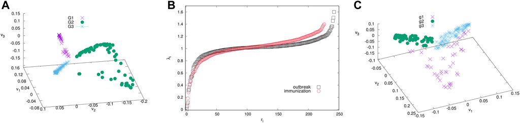
FIGURE 4. The ranking of eigenvalues of the normalised Laplacian for the outbreak and immunisation networks (B). Scatter plots of the eigenvectors v₁, v₂, v₃ corresponding to the three smallest non-zero eigenvalues for the outbreak (A) and immunisation period networks (C). Branches indicated by different colours identify the communities (groups) of nodes of the corresponding network in Figure 3.

Even though both networks exhibit three major communities, the structural differences between the two networks in Figure 3 are apparent. They indicate the corresponding differences in the fluctuations of the infection rates in the world regions during the immunisation phase, compared to the epidemic’s outbreak, when the whole population was practically susceptible to the infection. These differences are quantified by several graph measures, see Figures 2A–D and Table 1. Compatible with these graph-theory measures are the span of the exponentially-decaying degree distributions P_c(q) and different distributions of the shortest-path distances P(d), shown in Figure 2C. We also show the prominent differences in the q-core structure of these networks, cf. Figure 2D.

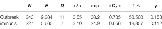
TABLE 1. For the outbreak and immunisation period networks: the number of nodes N, edges E, and triangles #△; the graph diameter D and density ρ; the average path length $<\ell >$, degree $<q>$, and clustering coefficient $<C_c>$.

More importantly, the majority of nodes that belong to the same community in the outbreak phase network appear to be a part of entirely different communities in the immunisation phase network, cf. Figure 3 and the corresponding lists in Supplementary Information. More precisely, we find that only 625 edges established in the outbreak phase persist in the immunisation phase network. They are shown in Supplementary Figure S2 left, in Supplementary Information. A more systematic comparison is made by computing the overlap (Jaccard index defined in Methods) for the correlation networks determined from the successive 2-month intervals, see Supplementary Figure S2, right. The overlap systematically remains below 15%, suggesting that the fluctuation patterns at these intervals can vary between the countries or even provinces within the same country.

2.6 K-Means Clustering and Multi-Fractality of Time Series Within Identified Communities

To further explore the nature of temporal fluctuations of the infection time series of the countries and provinces within each community found using spectral analysis, we apply the K-means algorithm adapted for time series analysis [58], see Methods. It appears that each topological community is further partitioned into several clusters, for example, G1c1⋯G1c4, for the group G1, and so on. Inside each cluster, the corresponding time series have a similar evolution pattern. Hence, the cluster’s typical time series (centroid) is determined for each identified cluster. The results are shown in Figure 5 both for the outbreak and immunisation phase; in the figure legends, the number of countries or provinces belonging to a given cluster is indicated in the brackets in each panel. The names of countries and provinces belonging to each cluster in each group are given in Supplementary Tables S1–S6 in Supplementary Information. Notably, in each network’s group, there is one large and one medium-size cluster. Meanwhile, there are several single-country centroids; as a rule, they indicate a large-population country.

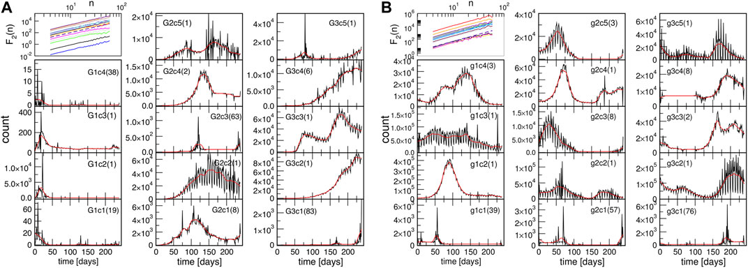
FIGURE 5. Centroids of clusters c1 to c5, found for three groups G1, G2 and G3, in the outbreak phase network (A), and groups g1, g2 and g3 in the immunisation phase network (B). In each panel, the number of countries and provinces belonging to that cluster is shown in brackets; the smooth red line represents the centroid’s trend. The top left panel in each figure shows the fluctuations function F₂(n) vs. segment length n for the identified trends; the slope h₂ = 2 is indicated by the dashed line.

Next we consider the fluctuation function F₂(n) vs. the interval length n for each time series separately, see some examples in Figure 6, and Supplementary Figure S4 in SI. We realised that the similarity of the time series belonging to each cluster manifests itself in the apparent similarity of the slopes of their fluctuation function, which defines the corresponding Hurst exponent. As Figure 6 shows, two different slopes of the fluctuation function can be identified for a majority of time series. At the intervals n < 14, a Hurst exponent 0.5 ≲ h₂ ≲ 1 can be determined, indicating persistent fluctuations occurring at these time intervals. Meanwhile, an exponent h₂ > 1, characteristic to the fractional Brownian motion, is found for n ≥ 14. In some cases, the determined Hurst exponent reaches values close to two. The histograms of the observed Hurst exponents are shown in Figures 6D,E. Compatible with the grouping and different shapes of centroids in the immunisation phase, the distributions of lower and higher values of the Hurts exponents are also different with the increased incidence of the value h₂ ≂ 0.5 (white noise), and h₂ ≂ 2 (periodic signals) in the immunisation phase. In the following, we show that these large values of the Hurst exponent in many of the studied time series can be related to the occurrence of cyclic trends.

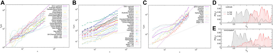
FIGURE 6. Examples of the standard deviation F₂(n) of time series vs. the interval length n for K-means clusters G1c1 and G3c1 identified within topological communities G1 and G3 in the outbreak (A,C), and cluster g2c3 in the immunisation phase networks (C). The distribution of the measured Hurst exponents for the intervals n < 14 days and n ≥ 14 days in the outbreak and immunisation phase (D,E).

Two prominent examples are shown in Figure 7. The methodology of determining local trends in these time series is described in Methods. The original time series shows a cyclic trend, where the cycle length can vary from region to region. A separate analysis of the fluctuation functions for the trend and the fluctuations around the local trend (detrended signal) reveals that the trend drives the fluctuations beyond the intervals of approximately 14 days; see the insets to Figure 7. The trend has true cyclic fluctuations (the Hurst exponent equals two, within error bars) in the range up to n ≲ 30 days. Meanwhile, beyond this range, both the original signal and trend have a lower Hurst exponent in the range h₂ ≳ 1, characterising a fractional Brownian motion. By extending a similar analysis to the above-mentioned typical time series (centroids), we find that they also exhibit cyclic trends but with different cycles characterising different clusters of countries. The corresponding trends are also shown in each panel of Figure 5 as a red line on the top of the related centroid. The trend fluctuation functions F₂(n) vs. n shows the cycle characteristics in a large range of the intervals n, cf. top left panels of Figure 5. They differ from cluster to cluster and, even for the same country, the cycles also differ in the outbreak and immunisation phase. Generally, larger cycles (in the length and amplitude) are observed in the immunisation phase as compared to the outbreak period, cf. Supplementary Figure S5 in SI. Remarkably, these findings imply that the cycles (or the infection waves) represent an inherent feature of current pandemic which may have some long-lasting consequences.

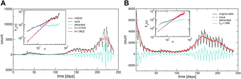
FIGURE 7. Two examples of the infection time series showing cyclic trends during the outbreak phase [from Israel, (A)], and during the immunisation phase [from Portugal, (B)]. Insets show the corresponding functions of the standard deviation fluctuations for the identified trends and the original and detrended time series.

3 Discussion and Conclusion

In search of universal characteristics of infection dynamics, we have analysed the worldwide empirical data of the SARS-CoV-2 epidemic [44], focusing on the new-infection time series with a daily resolution. The data are purposefully divided into two periods, corresponding to the epidemic’s outbreak and the initial immunisation phase, respectively. Three complementary methods of quantitative analysis have been performed. Specifically, we have analysed the mesoscopic structure of the networks, which embody the significant pairwise correlations among the infection time series of different countries or provinces. The further similarity in the pairs of time series has been analysed by K-means clustering. Finally, the fluctuation function of each time series has been determined using the detrended time series analysis. Our analysis has revealed global clustering and several universal features of the infection dynamics. Our main conclusions are:

• the worldwide clustering represented by fourteen temporal patterns of evolution of infection reveals significant similarities transcending geographical regions;

• the cyclic trends dominate the infection fluctuations, implying the prevalent infection waves and multi-scale fluctuations around these cycles; typically determined cycles appear in conjunction with the identified clusters;

• the immunisation phase differs from the epidemic outbreak phase in all measures considered here, thus quantifying the impact of the (partial) immunisation coverage on the underlying stochastic process and the course of the pandemic.

The mesoscopic (community) structure, as shown in Figure 3 is one of the striking characteristics of the infection-correlation networks; remarkably, it occurs already at zero thresholds, see Supplementary Figure S1 in SI. What comes as a surprise is that these communities constitute almost entirely different nodes (countries or provinces) in the immunisation phase compared to the outbreak phase. Only a few edges established during the outbreak phase persist throughout the entire evolution of the epidemic, as shown in Supplementary Figure S2 in SI. Consequently, the same applies to the contents of the clusters found in these two phases, cf. Supplementary Tables S1–S6 in SI. Notably, a given geographic location and potentially similar cultural and economic development levels, similar healthcare systems and other related factors play some role. However, even such regional groups appear to be a part of a worldwide cluster in both representative phases of the pandemic. Such a picture probably emerges under another dominant driver, common to countries at different locations, and with different cultural and economic developments. In this context, the biology factors, the virus mutations in the interplay with the social behaviour of individuals and groups in the crisis seems to be of the primary importance for the genesis of sustained infection waves, quantified by cyclic trends in different clusters, cf. Figure 7. Our analysis suggests that the waves are ubiquitous in all countries and regions in both representative phases of the pandemic. Meanwhile, the timing, duration and amplitude of these waves vary between different clusters of countries and provinces, likely depending on the applied measures and the corresponding variations in the population behaviours. Moreover, the small-scale fluctuations around these cyclic trends seem to be more region-specific, and depending on the immunisation measures; two comparative examples are shown in Supplementary Figure S5 in SI. A more systematic analysis of these fluctuations and the impact of the immunisation level on the infection dynamics merits future study.

Our analysis of the world infection dynamics of the SARS-CoV-2 pandemic revealed several universal features of the underlying multiscale stochastic processes that go beyond the geographical impact, locally-imposed governmental measures, and partial immunisation phases. Indeed, while these measures are truly valuable for short-term effects, saving lives, and maintaining the functional healthcare system in each country [25], they are much less effective in changing the fundamental nature of the infection process, rooted in the interplay of biology and social behaviours. This work has provided an in-depth analysis of the pandemic’s fundamental phases with an overview that can guide further research into the nature of biosocial interdependencies. The latter factor plays a critical role in the SARS-CoV-2 evolution, where individual biological features of the participants and their role in the collective behaviours need to be better understood. Our effective long-term management of the pandemic and prediction of its future developments rely upon our ability to continue unfolding critical attributes of the underlying biosocial stochastic dynamics.

Data Availability Statement

Publicly available datasets were analyzed in this study. This data can be found here: https://github.com/CSSEGISandData/COVID-19/.

Author Contributions

BT, RM, and MM designed research, MM collected data, MM and BT contributed program tools and performed analysis, BT, MM, and RM analysed data, BT produced figures, BT and RM wrote the manuscript, all authors reviewed the manuscript.

Funding

BT work supported by the Slovenian Research Agency (research code funding number P1-0044). MMD. acknowledge funding provided by the Institute of Physics Belgrade, through the grant by the Ministry of Education, Science, and Technological Development of the Republic of Serbia. RM is grateful to the NSERC and the CRC Program for their support and he is also acknowledging the support of the BERC 2022-2025 program and Spanish Ministry of Science, Innovation, and Universities through the Agencia Estatal de Investigacion (AEI) BCAM Severo Ochoa excellence accreditation SEV-2017-0718, and the Basque Government fund AI in BCAM EXP. 2019/00432.

Conflict of Interest

The authors declare that the research was conducted in the absence of any commercial or financial relationships that could be construed as a potential conflict of interest.

Publisher’s Note

All claims expressed in this article are solely those of the authors and do not necessarily represent those of their affiliated organizations, or those of the publisher, the editors and the reviewers. Any product that may be evaluated in this article, or claim that may be made by its manufacturer, is not guaranteed or endorsed by the publisher.

Supplementary Material

The Supplementary Material for this article can be found online at: https://www.frontiersin.org/articles/10.3389/fphy.2022.936618/full#supplementary-material

References

1. Jusup M, Holme P, Kanazawa K, Takayasu M, Romić I, Wang Z, et al. Social Physics. Phys Rep (2022) 948:1–148. doi:10.1016/j.physrep.2021.10.005
2. Perc M, Jordan JJ, Rand DG, Wang Z, Boccaletti S, Szolnoki A. Statistical Physics of Human Cooperation. Phys Rep (2017) 687:1–51. doi:10.1016/j.physrep.2017.05.004
3. Tadić B, Melnik R. Self-organised Critical Dynamics as a Key to Fundamental Features of Complexity in Physical, Biological, and Social Networks. Dynamics (2021) 1:181–97.
4. Tadić B, Dankulov MM, Melnik R. Mechanisms of Self-Organized Criticality in Social Processes of Knowledge Creation. Phys Rev E (2017) 96:032307. doi:10.1103/PhysRevE.96.032307
5. Chilamakuri R, Agarwal S. Covid-19: Characteristics and Therapeutics. Cells (2021) 10:206. doi:10.3390/cells10020206
6. Gerotziafas GT, Catalano M, Theodorou Y, Dreden PV, Marechal V, Spyropoulos AC, et al. The Covid-19 Pandemic and the Need for an Integrated and Equitable Approach: an International Expert Consensus Paper. Thromb Haemost (2021) 121:992–1007. doi:10.1055/a-1535-8807
7. Hâncean MG, Slavinec M, Perc M. The Impact of Human Mobility Networks on the Global Spread of Covid-19. J Complex Networks (2020) 8:cnaa041.
8. Tadić B, Melnik R. Modeling Latent Infection Transmissions through Biosocial Stochastic Dynamics. PloS one (2020) 15:e0241163. doi:10.1371/journal.pone.0241163
9. Doms RW. Basic Concepts. In: Viral Pathogenesis. Amsterdam: Elsevier (2016). p. 29–40. doi:10.1016/b978-0-12-800964-2.00003-3
10. Schneider M, Johnson JR, Krogan NJ, Chanda SK. The Virus-Host Interactome. In: Viral Pathogenesis. Amsterdam: Elsevier (2016). p. 157–67. doi:10.1016/b978-0-12-800964-2.00012-4
11. Callaway E. The Coronavirus Is Mutating - Does it Matter? Nature (2020) 585:174–7. doi:10.1038/d41586-020-02544-6
12. Lu C, Gam R, Pandurangan AP, Gough J. Genetic Risk Factors for Death with Sars-Cov-2 from the uk Biobank. MedRxiv (2020). doi:10.1101/2020.07.01.20144592
13. Zhang Y, Geng X, Tan Y, Li Q, Xu C, Xu J, et al. New Understanding of the Damage of Sars-Cov-2 Infection outside the Respiratory System. Biomed Pharmacother (2020) 127:110195. doi:10.1016/j.biopha.2020.110195
14. Cevik M, Kuppalli K, Kindrachuk J, Peiris M. Virology, Transmission, and Pathogenesis of Sars-Cov-2. BMJ (2020) 371:m3862. doi:10.1136/bmj.m3862
15. Meyers KJ, Jones ME, Goetz IA, Botros FT, Knorr J, Manner DH, et al. A Cross‐sectional Community‐based Observational Study of Asymptomatic SARS‐CoV‐2 Prevalence in the Greater Indianapolis Area. J Med Virol (2020) 92:2874–9. doi:10.1002/jmv.26182
16. Chen J. Pathogenicity and Transmissibility of 2019-nCoV-A Quick Overview and Comparison with Other Emerging Viruses. Microbes Infect (2020) 22:69–71. doi:10.1016/j.micinf.2020.01.004
17. Wang Y, Wang Y, Chen Y, Qin Q. Unique Epidemiological and Clinical Features of the Emerging 2019 Novel Coronavirus Pneumonia (COVID‐19) Implicate Special Control Measures. J Med Virol (2020) 92:568–76. doi:10.1002/jmv.25748
18. Djordjevic M, Salom I, Markovic S, Rodic A, Milicevic O, Djordjevic M. Inferring the Main Drivers of Sars-Cov-2 Global Transmissibility by Feature Selection Methods. GeoHealth (2021) 5:e2021GH000432. doi:10.1029/2021GH000432
19. Bavel JJV, Baicker K, Boggio PS, Capraro V, Cichocka A, Cikara M, et al. Using Social and Behavioural Science to Support Covid-19 Pandemic Response. Nat Hum Behav (2020) 4:460–71. doi:10.1038/s41562-020-0884-z
20. Chaudhry R, Dranitsaris G, Mubashir T, Bartoszko J, Riazi S. A Country Level Analysis Measuring the Impact of Government Actions, Country Preparedness and Socioeconomic Factors on Covid-19 Mortality and Related Health Outcomes. EClinicalMedicine (2020) 25:100464. doi:10.1016/j.eclinm.2020.100464
21. Funk CD, Laferrière C, Ardakani A. A Snapshot of the Global Race for Vaccines Targeting Sars-Cov-2 and the Covid-19 Pandemic. Front Pharmacol (2020) 11:937. doi:10.3389/fphar.2020.00937
22. Wang Z, Bauch CT, Bhattacharyya S, d'Onofrio A, Manfredi P, Perc M, et al. Statistical Physics of Vaccination. Phys Rep (2016) 664:1–113. doi:10.1016/j.physrep.2016.10.006
23. Khajanchi S, Das DK, Kar TK. Dynamics of Tuberculosis Transmission with Exogenous Reinfections and Endogenous Reactivation. Physica A: Stat Mech its Appl (2018) 497:52–71. doi:10.1016/j.physa.2018.01.014
24. Khajanchi S, Perc M, Ghosh D. The Influence of Time Delay in a Chaotic Cancer Model. Chaos (2018) 28:103101. doi:10.1063/1.5052496
25. Haug N, Geyrhofer L, Londei A, Dervic E, Desvars-Larrive A, Loreto V, et al. Ranking the Effectiveness of Worldwide Covid-19 Government Interventions. Nat Hum Behav (2020) 4:1303–12. doi:10.1038/s41562-020-01009-0
26. Weitz JS, Park SW, Eksin C, Dushoff J. Awareness-driven Behavior Changes Can Shift the Shape of Epidemics Away from Peaks and toward Plateaus, Shoulders, and Oscillations. Proc Natl Acad Sci U.S.A (2020) 117:32764–71. doi:10.1073/pnas.2009911117
27. Tkachenko AV, Maslov S, Elbanna A, Wong GN, Weiner ZJ, Goldenfeld N. Time-dependent Heterogeneity Leads to Transient Suppression of the Covid-19 Epidemic, Not Herd Immunity. Proc Natl Acad Sci (2021) 118. doi:10.1073/pnas.2015972118
28. Brauer F. Mathematical Epidemiology: Past, Present, and Future. Infect Dis Model (2017) 2:113–27. doi:10.1016/j.idm.2017.02.001
29. Tadić B, Melnik R. Microscopic Dynamics Modeling Unravels the Role of Asymptomatic Virus Carriers in Sars-Cov-2 Epidemics at the Interplay between Biological and Social Factors. Comput Biol Med (2021) 133:104422. doi:10.1016/j.compbiomed.2021.104422
30. Nagel K, Rakow C, Müller SA. Realistic Agent-Based Simulation of Infection Dynamics and Percolation. Physica A: Stat Mech its Appl (2021) 584:126322. doi:10.1016/j.physa.2021.126322
31. Burda Z. Modelling Excess Mortality in Covid-19-like Epidemics. Entropy (2020) 22:1236. doi:10.3390/e22111236
32. Chang SL, Harding N, Zachreson C, Cliff OM, Prokopenko M. Modelling Transmission and Control of the Covid-19 Pandemic in australia. Nat Commun (2020) 11:5710–3. doi:10.1038/s41467-020-19393-6
33. Jackson ML. Low-impact Social Distancing Interventions to Mitigate Local Epidemics of Sars-Cov-2. Microbes Infect (2020) 22:611–6. doi:10.1016/j.micinf.2020.09.006
34. Lin Q, Zhao S, Gao D, Lou Y, Yang S, Musa SS, et al. A Conceptual Model for the Coronavirus Disease 2019 (Covid-19) Outbreak in Wuhan, china with Individual Reaction and Governmental Action. Int J Infect Dis (2020) 93:211–6. doi:10.1016/j.ijid.2020.02.058
35. Magal P, Webb G. Predicting the Number of Reported and Unreported Cases for the Covid-19 Epidemic in south korea, italy, france and germany (2020). Italy, France and Germany (March 19, 2020).
36. Hoertel N, Blachier M, Blanco C, Olfson M, Massetti M, Rico MS, et al. A Stochastic Agent-Based Model of the Sars-Cov-2 Epidemic in france. Nat Med (2020) 26:1417–21. doi:10.1038/s41591-020-1001-6
37. Rice BL, Annapragada A, Baker RE, Bruijning M, Dotse-Gborgbortsi W, Mensah K, et al. Variation in Sars-Cov-2 Outbreaks across Sub-saharan Africa. Nat Med (2021) 27:447–53. doi:10.1038/s41591-021-01234-8
38. Giordano G, Blanchini F, Bruno R, Colaneri P, Di Filippo A, Di Matteo A, et al. Modelling the Covid-19 Epidemic and Implementation of Population-wide Interventions in italy. Nat Med (2020) 26:855–60. doi:10.1038/s41591-020-0883-7
39. Anastassopoulou C, Russo L, Tsakris A, Siettos C. Data-based Analysis, Modelling and Forecasting of the Covid-19 Outbreak. PloS one (2020) 15:e0230405. doi:10.1371/journal.pone.0230405
40. Christopoulos DT. A Novel Approach for Estimating the Final Outcome of Global Diseases like Covid-19. medRxiv (2020). doi:10.1101/2020.07.03.20145672
41. Thurner S, Klimek P, Hanel R. A Network-Based Explanation of Why Most Covid-19 Infection Curves Are Linear. Proc Natl Acad Sci U.S.A (2020) 117:22684–9. doi:10.1073/pnas.2010398117
42. Vasconcelos GL, Macêdo AMS, Duarte-Filho GC, Brum AA, Ospina R, Almeida FAG. Power Law Behaviour in the Saturation Regime of Fatality Curves of the Covid-19 Pandemic. Sci Rep (2021) 11:4619–2. doi:10.1038/s41598-021-84165-1
43. Tkachenko AV, Maslov S, Wang T, Elbana A, Wong GN, Goldenfeld N. Stochastic Social Behavior Coupled to Covid-19 Dynamics Leads to Waves, Plateaus, and an Endemic State. Elife (2021) 10:e68341. doi:10.7554/eLife.68341
44.[Dataset] CSSE. Covid-19 Data Repository by the center for Systems Science and Engineering (Csse) at the Johns hopkins university (2020).
45. Plerou V, Gopikrishnan P, Rosenow B, Amaral LAN, Stanley HE. Econophysics: Financial Time Series from a Statistical Physics point of View. Physica A: Stat Mech its Appl (2000) 279:443–56. doi:10.1016/s0378-4371(00)00010-8
46. Maslov S. Measures of Globalization Based on Cross-Correlations of World Financial Indices. Physica A: Stat Mech its Appl (2001) 301:397–406. doi:10.1016/s0378-4371(01)00370-3
47. Tadić B, Mitrović M. Jamming and Correlation Patterns in Traffic of Information on Sparse Modular Networks. The Eur Phys J B (2009) 71:631–40.
48. Isufaj R, Koca T, Piera MA. Spatiotemporal Graph Indicators for Air Traffic Complexity Analysis. Aerospace (2021) 8:364. doi:10.3390/aerospace8120364
49. Baruchi I, Ben-Jacob E. Functional Holography of Recorded Neuronal Networks Activity. Ni (2004) 2:333–52. doi:10.1385/ni:2:3:333
50. Tadić B, Andjelković M, Boshkoska BM, Levnajić Z. Algebraic Topology of Multi-Brain Connectivity Networks Reveals Dissimilarity in Functional Patterns during Spoken Communications. PLoS One (2016) 11:e0166787. doi:10.1371/journal.pone.0166787
51. Madi A, Friedman Y, Roth D, Regev T, Bransburg-Zabary S, Jacob EB. Genome Holography: Deciphering Function-form Motifs from Gene Expression Data. PLoS One (2008) 3:e2708. doi:10.1371/journal.pone.0002708
52. Živković J, Tadić B, Wick N, Thurner S. Statistical Indicators of Collective Behavior and Functional Clusters in Gene Networks of Yeast. Eur Phys J B-Condensed Matter Complex Syst (2006) 50:255–8.
53. Lahiri D, Dubey S, Ardila A. Impact of Covid-19 Related Lockdown on Cognition and Emotion: A Pilot Study. medRxiv (2020). 2020.06.30.20138446. doi:10.1101/2020.06.30.20138446
54. Browning R, Sulem D, Mengersen K, Rivoirard V, Rousseau J. Simple Discrete-Time Self-Exciting Models Can Describe Complex Dynamic Processes: A Case Study of Covid-19. PloS one (2021) 16:e0250015. doi:10.1371/journal.pone.0250015
55. Biyikoglu T, Leydold J, Stadler PF. Laplacian Eigenvectors of Graphs: Perron-Frobenius and Faber-Krahn Type Theorems. Heidelberg: Springer (2007).
56. Mitrović M, Tadić B. Spectral and Dynamical Properties in Classes of Sparse Networks with Mesoscopic Inhomogeneities. Phys Rev E (2009) 80:026123.
57. Bastian M, Heymann S, Jacomy M. Gephi: an Open Source Software for Exploring and Manipulating Networks. Proc Int AAAI Conf web Soc media (2009) 3:361–2.
58. Tavenard R, Faouzi J, Vandewiele G, Divo F, Androz G, Holtz C, et al. Tslearn, a Machine Learning Toolkit for Time Series Data. J Mach Learn Res (2020) 21:1–6.
59. Hu J, Gao J, Wang X. Multifractal Analysis of sunspot Time Series: the Effects of the 11-year Cycle and Fourier Truncation. J Stat Mech (2009) 2009:P02066. doi:10.1088/1742-5468/2009/02/p02066
Keywords: complex networks, k-means, time-series analysis, spectral analysis, community structure, SARS-CoV-2
Citation: Mitrović Dankulov M, Tadić B and Melnik R (2022) Analysis of Worldwide Time-Series Data Reveals Some Universal Patterns of Evolution of the SARS-CoV-2 Pandemic. Front. Phys. 10:936618. doi: 10.3389/fphy.2022.936618
Received: 05 May 2022; Accepted: 23 May 2022;
Published: 29 June 2022.
Edited by:
Matjaž Perc, University of Maribor, SloveniaReviewed by:
Marian-Gabriel Hancean, University of Bucharest, RomaniaNuno A. M. Araújo, University of Lisbon, Portugal
Yinhai Fang, Nanjing Forestry University, China
Copyright © 2022 Mitrović Dankulov, Tadić and Melnik. This is an open-access article distributed under the terms of the Creative Commons Attribution License (CC BY). The use, distribution or reproduction in other forums is permitted, provided the original author(s) and the copyright owner(s) are credited and that the original publication in this journal is cited, in accordance with accepted academic practice. No use, distribution or reproduction is permitted which does not comply with these terms.
*Correspondence: Marija Mitrović Dankulov, mitrovic@ipb.ac.rs