Estimating Parameters of Two-Level Individual-Level Models of the COVID-19 Epidemic Using Ensemble Learning Classifiers

Introduction

The COVID-19 epidemic [1, 2] has caused the most serious threat to global health since the early 20th century; the exponential spread of the SARS-CoV-2 virus around the world has caused over 26 million confirmed cases and 860 thousand deaths worldwide as reported by the John Hopkins University COVID-19 web dashboard (https://coronavirus.jhu.edu/map.html) at the time of writing [3]. The spread of the SARS-CoV-2 virus, which causes COVID-19, has varied considerably in different areas, in part depending on the control different measures taken. Intensive testing, tracing, and isolation of infected cases have enabled control of transmission in some places, such as China and Singapore [4]. At the opposite extreme, many countries lack the testing and public health resources to take similar measures to control the COVID-19 epidemic, which can result in unhindered spread. Between these extremes, many countries have taken measures that facilitate “social distancing”, such as closing schools and workplaces and limiting the size of gatherings. In order to analyze the dynamics of COVID-19 outbreak, we build an epidemic model based on the individual-level model (ILM) of Deardon et al (2010) [5] to catch the spread of SARS-CoV-2 virus within and among cities.

The individual-level model (ILM) framework enables us to express the probability of a susceptible individual being infected at a point in discrete time, as a function of their interactions with the surrounding infectious population, while also allowing the incorporation of the effect of individually varying risk factors. Here, we consider an extension of the Deardon et al (2010) framework of ILMs, to allow the probability of infection to depend upon two levels of transmission dynamics. The first is a within-city (or region) level; the second is a between-city level. Infectious diseases are generally modeled through compartmental frameworks, and here we place our ILMs within the susceptible-infectious-removed (SIR) framework [6]. In the SIR framework, infected individuals become instantly infectious upon exposure, with no dormant or latent period. Since, in reality, infection is not observed instantaneously, and many infected individuals are not recorded at all in the data, we add an “observation model” which ties the epidemic generating model above to the observed data. This consists of a geometric distribution-based “delay model” and a “reporting model” which assumes that the probability of a true case being reported follows a Bernoulli distribution.

ILMs are intuitive and flexible due to being expressed in terms of individual interactions [7–9], but the cost of computation to parameterize them using observed data is often expensive, especially when dealing with a disease spreading in large populations. Traditional parameter estimation methods, such as Bayesian Markov chain Monte Carlo, have an associated high computation cost. Recent works by Nsoesie et al (2011) [10], Pokharel et al (2014) [11], and Augusta et al (2019) [12] have shown how to bypass the likelihood calculations by using machine learning classifiers to fit ILMs to data. In this work, we develop this approach to explore the use of ensemble learning classifiers to accurately and efficiently find the parameters for our two-level ILM, which incorporates a delay and reporting mechanism.

Generating Model

In this section, we present the two-level epidemic ILM [13] and observation model (delay model and reporting model) which ties the epidemic model to observed data. We denote the set of individuals who are susceptible, infectious, or removed at time $t$ in city/region k as $S_{k,t}$, $I_{k,t}$, or $R_{k,t}$, respectively. Note, for given $t$, these sets are mutually exclusive, so individuals cannot be in multiple states, or multiple cities. Here, we assume time is discretized so that time point $t$, for $t=1, 2, \mathrm{...}n$, represents a continuous time interval $[t, t+1)$.

Two-Level Individual-Level Model

The number of newly infectious persons in city $k$ at time point $t+1$ is given by

where $\left|S_{k,t}\right|$ is the number of susceptible individuals within city $k$ at time $t$, and $P_{k,t}$ is the probability of each susceptible individual in the $k^{th}$ city being infected at time $t$. Here, $P_{k,t}$ is given by

where $n$ is the number of cities in the population; $\left|I_{k,t}\right|$ is the number of infectious individuals within city $k$ at time $t$; $\alpha$ is a parameter representing the risk of infection within cities; and ${\alpha }_1$ and $\beta$ are parameters representing the risk of infection between cities, with $\beta$ capturing the decay rate of a power-law distance-based kernel, $d_{k,j}^{-\beta }$. Note, decreasing $\beta$ will lead to a lower rate of decay in the infection kernel and thus more long-distance infections.

In the two-level ILM-SIR model, the transitions from susceptible to infectious and from infectious to recovered are treated as events of interest. In this work, the number of time points (days) between $I$ and $R$ is referred to as the infectious period, denoted by $\gamma$. The constant infectious period expresses the number of days over which an infectious individual is capable of transmitting the disease.

Observation Model

Here, we consider adding an observation model which ties epidemics generated by epidemic model to observed data.

Delay Model

Since there is a delay between infection and observation of that infection (reporting), we use a delay model to better represent reality. Specifically, given true infection times ${\tau }_i\in {\text{Ζ}}^{+}$ for each infected individual $i$, we let the potential observation time for individual $i$ to be

where $P^D$ is the delay rate parameter. Note ${\tau }_i^D$ is a potential observation time, since case $i$ may not be observed at all.

Reporting Model

The second component of the observation model, the “reporting model”, accounts for asymptomatic, or otherwise unreported, cases of COVID-19. Here, we assume the probability of observing a case and it being recorded in the data (at time ${\tau }_i^D$) follows a Bernoulli distribution, such that

where $P^R$ is the reporting rate parameter.

Ensemble Learning Classifiers

In supervised learning algorithms, the goal is to learn a stable classification (or regression) model that performs well across a wide range of data scenarios. Often, however, this is a difficult goal to achieve. Ensemble learning is the process by which multiple models are strategically “learned” and combined to solve a computational intelligence problem. Ensemble learning is primarily used to provide for an improved performance over any single model, or to reduce the likelihood of the selection of a poor single model. Bagging, boosting, and stacking are common ensemble learning algorithms. Note, here, we are concerned with classification rather than regression problems.

Bagging

Bagging, which stands for bootstrap aggregating, is one of the earliest, most intuitive, and perhaps the simplest ensemble based algorithms, with a surprisingly good performance [14]. A diversity of classifiers in bagging is obtained by using bootstrapped replicas of the training data. That is, different training data subsets are randomly drawn—with replacement—from the entire training dataset. Each training data subset is used to train a different classifier of the same type. Individual classifiers are then combined by taking a simple majority vote of their decisions. For any given instance, the class chosen by the greatest number of classifiers is the ensemble decision.

The random forest is a bagging method for trees, later extended to incorporate random selection of features to help control variance [15, 16].

Boosting

Similar to bagging, boosting also creates an ensemble of classifiers by resampling the data, which are then combined by majority voting. However, in boosting, resampling is strategically geared to provide the most informative training data for each consecutive classifier.

The gradient boosted decision tree (GBDT) method [17–19] uses decision trees as the base learner and sums the predictions of a series of trees. At each step, a new decision tree is trained to fit the residuals between ground truth and the current prediction. Many improvements have since been proposed. XGBoost [20] uses a second-order gradient to guide the boosting process and improve the accuracy. LightGBM [21] aggregates gradient information in histograms to significantly improve the training efficiency; it splits the tree leaf-wise with the best fit, whereas other boosting algorithms split the tree depth-wise or level-wise rather than leaf-wise. AdaBoost, short for Adaptive Boosting, can be used in conjunction with many other types of learning algorithms to improve performance; the output of the other learning algorithms (weak learners) is combined into a weighted sum that represents the final output of the boosted classifier. Finally, CatBoost [22] proposed a novel strategy to deal with categorical features.

Stacking

Stacking, sometimes called stacked generalization, is also an ensemble learning method that combines multiple classification (or regression) models via a metaclassifier or a metaregressor. The base level models are trained based on a complete training set; then the metamodel is trained on the outputs of the base level model as features. Stacking involves training a learning algorithm to combine the predictions of several other learning algorithms. Stacking typically yields performance better than any single one of the trained models [23]. It has been successfully used on both supervised learning tasks (regression, classification, and distance learning) and unsupervised learning (density estimation).

Experiment

Typically, ILMs are fitted to data using computationally intensive techniques such as Bayesian Markov chain Monte Carlo methods. In order to avoid this computational expense, in this study we use the method of Pokharel et al (2014) to fit our models to data. Broadly this method involves defining a set of candidate generating models, each with different parameter values. Then, epidemics are repeatedly generated from the candidate models and summarized. Here, we summarize the epidemics using the number of observed cases per day, what we term the “epidemic curve”. These epidemic curve summary statistics form the training set used to build a classifier mapping the epidemic curve (input features) to the generating model (class). The classifier can then be used to identify the most likely generating model for future observed summaries of epidemic data sets; several ensemble learning classifiers such as random forest, XGBoost, LightGBM, AdaBoost, CatBoost, and stacking are used to seek the best fitted parameter for the two-level ILM model. Here, we verify the accuracy of these ensemble learning classifiers by testing their performance on data simulated from the two-level ILM model. In Real Data Case Study: COVID-19 in Hubei Province, China, we will use such classifiers to estimate the parameters that give the model of best fit when applied to COVID-19 data from Hubei province, China.

Simulation Study

We now recap the parameters we need to identify: ${\alpha }_0$, $\beta$, and ${\alpha }_1$ are the parameters of the two-level epidemic model in Eq. 2; $t_{stop}$ is the interval of time from the initial infection (unknown) to the day when the epidemic stopped by external intervention (lockdown) in Hubei province; $\gamma$ is the infectious period, assumed to be constant for all individuals; $p^D$ is the rate parameter of the delay model; and $p^R$ is the rate parameter of the reporting model. Here we assume that when day $t=t_{stop}$ is reached, the rate of new infections becomes negligible, and so ${\alpha }_0={\alpha }_1=0$. Thus, newly observed cases after day $t=t_{stop}$ result from earlier infections becoming observed through the delay model.

In the simulation experiment, we suppose there are total 100 cities, where (x,y) coordinates are simulated uniformly across a 100 $\times$ 100 unit. Further, the population of each city is set at 1,000. Each candidate two-level ILM is used to generate 100 epidemics, summarized as epidemic curves. To initialize the SIR model, we set the value of $I_0$ to 50 in the one city (chosen randomly), where the disease originates. Here, a maximum of 12 candidate epidemic generating models are considered in each analysis with parameters shown in Table 1. Sets of generated epidemic curves are shown in Figure 1, with different colors denoting different epidemic generating models.

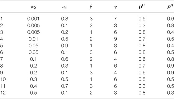
TABLE 1. The parameters of ILM generating model.

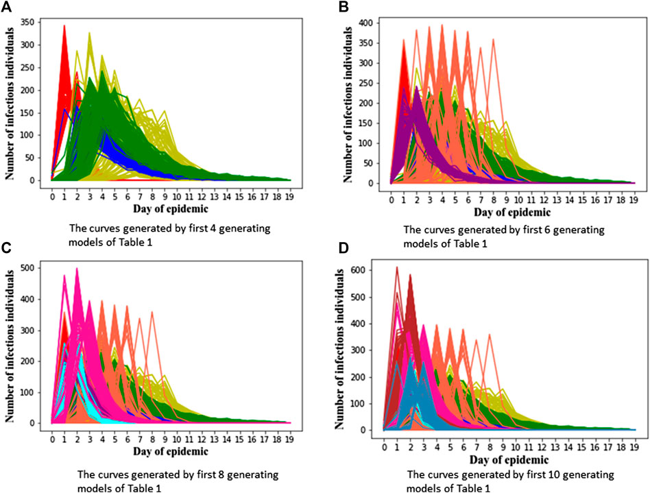
FIGURE 1. Epidemic curves generated under various training sets.

In order to verify the performance of classifiers, we have carried out five classification tasks, each consisting of different numbers of epidemic generating models. These tasks consisted of the first 4, 6, 8, 10, and 12 models of Table 1, respectively. The generated data is randomly divided into a training set and test set, with 70% of the data for the training set, and the rest for the test set. The results of classification are shown in Tables 2, 3.

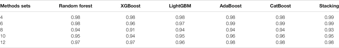
TABLE 2. The accuracy of different classifiers for training sets of 70 curves per generating model.

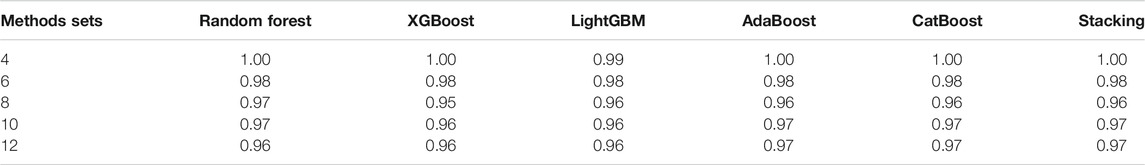
TABLE 3. The accuracy of different classifiers for training sets of 140 curves per generating model.

We can see Figure 1 has epidemic curves that overlap substantially. However, all classifiers achieve quite high accuracy. We also repeated the simulation study using 200 curves per epidemic generating model (140 training; 60 test). The results are shown in Table 3, and we can see that accuracy increases when we have larger training sets.

The details of super-parameters of classifiers used to get the best classification score are as follows. The parameters in AdaBoost classifier are as follows: the max depth is 6, the number of estimators is 1,000, and the learning rate is 0.008; the parameters in CatBoost classifier are as follows: the depth is 6, the iteration is 1,200, and the learning rate is 0.05; the parameters in LightGBM classifier are as follows: the max depth is 8, the number of estimators is 150, and the learning rate is 0.05; the parameters in random forest classifier are as follows: the max depth is 8, the number of estimators is 300; the parameters in XGBoost classifier are as follows: the max depth is 10, the number of estimators is 250, and the learning rate is 0.1.

Real Data Case Study: COVID-19 in Hubei Province, China

We now consider training a classifier to find the parameters of best fit for the two-level ILM for COVID-19 data from China. As the first reported COVID-19 cases happened in the city of Wuhan, we choose the Hubei province in China as the example in this study. There are in total 17 cities in Hubei province, and we utilize information on the population of each city and the distance between cities for the two-level epidemic ILM.

For the distance between each city, we use the center of each city as its coordinate point, and then we choose to use the shortest road traffic distance based on Baidu map (https://map.baidu.com). Rather than using the total population size to calculate the terms $\left|S_{k,t}\right|$ and $\left|I_{k,t}\right|$, we consider using the population in the central urban area (where most citizens live). Further, we scaled the population of each city based on the ratio of population density in central urban area relative to that in Wuhan. Thus, the population measure of each of the other 16 cities in Hubei will be greater or less than one depending on whether their population density in central urban area is greater or less than that of Wuhan. These measures of population density are shown in Table 4 (adjusted population column).

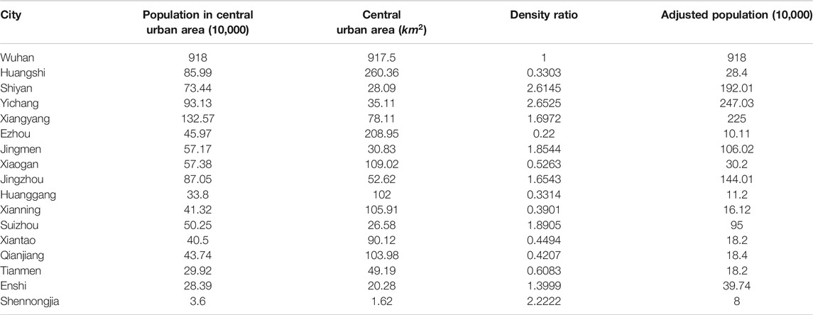
TABLE 4. Adjusted population of 17 cities in Hubei.

The reported case data had some anomalies, and so some preprocessing was carried out. For example, the number of new cases in Wuhan on February 12, 2020, was recorded as more than ten thousand, which is much larger than on other days. Also, there were two other cities which had a two-day spike of an excessively large magnitude. We believe these spikes represent retrospectively found cases, which should have been recorded as cases on earlier days, “dumped into the data” on those “spike” days. Further, some values in the reported data were negative because the health agencies subtracted retrospectively discovered false positives from the date on which the false positives were discovered, rather than the day on which they were initially recorded. For the large one-day spike, we took the average of values of three days before and three days after the spike and used this average value to replace the spike case count. Then we “scattered” the excess cases onto past days, at a rate proportional to the previously observed cases recorded on each day. The two-day spikes were replaced in a similar manner, the difference being that in this case two spikes were replaced by the average value. For negative values, we simply replaced them with zero. Our preprocessed data can be found in the Supplementary Tables S1, S2.

We build our classifier in the following way. To begin, we consider epidemic generating models that are relatively spaced out in the parameter space. We initially set the range of parameter ${\alpha }_0$ from $5\times {10}^{-8}$ to $5\times {10}^{-6}$, the range of ${\alpha }_1$ from $0.0005$ to $0.05$, the range of $\beta$ from $1$ to $9$, the range of $t_{stop}$ from $40$ to $100$, the range of $\gamma$ from $10$ to $30$, the range of $p^R$ from $0.1$ to $0.7$, and the range of $p^D$ from $0.4$ to $1$. Specifically, for ${\alpha }_0$, we consider values of $5\times {10}^{-8}$, $5\times {10}^{-7}$, and $5\times {10}^{-6}$; for ${\alpha }_1$, we set the values to be 0.0005, 0.005, and 0.05. We set the step size of $\beta$ to be 4 (i.e., we considered values 1,5, and 9), the step size of $t_{stop}$ to be 30, the step size of $\gamma$ to be 10, and the step size of $p^D$ and $p^R$ to be 0.3. Thus, we have $3^7$ epidemic generating models. We build our classifier based upon epidemics generated by each model and then use the Adaboost classifier to identify which of the candidate models is the most likely generating model for the real data.

After the first round of classification, the most likely generating model is found to be one with parameters: ${\alpha }_0=5\times {10}^{-8}$, ${\alpha }_1=0.005$, $\beta =1$, $t_{stop}=70$, $\gamma =20$, $p^D=0.4$, and $p^R=0.7$. Next, a less spaced-out set of parameter values are considered to define the generating models. We set the range of ${\alpha }_0$ from $2\times {10}^{-8}$ to $8\times {10}^{-8}$, the range of ${\alpha }_1$ from $0.002$ to $0.008$, the range of $\beta$ from $0.5$ to $3.5$, the range of $t_{stop}$ from $55$ to $85$, the range of $\gamma$ from $15$ to $25$, the range of $p^D$ from $0.2$ to $0.6$, and the range of $p^R$ from $0.5$ to $0.9$. We set the step size of ${\alpha }_0$ to be $3\times {10}^{-8}$, the step size of ${\alpha }_1$ to be 0.003, the step size of $\beta$ to be 1.5, the step size of $t_{stop}$ to be 15, the step size of $\gamma$ to be 5, the step size of $p^D$ to be 0.2, and the step size of $p^R$ to be 0.2. The parameters of the most likely generating model we get in this second round are ${\alpha }_0=2\times {10}^{-8}$, ${\alpha }_1=0.002$, $\beta =2$, $t_{stop}=70$, $\gamma =15$, $p^D=0.4$, and $p^R=0.7$. As the approach continues, parameters of candidate generating models obviously get closer and closer to each other, with generated curves overlapping more and more and classification becoming less well defined. After six rounds of classification, we converge on estimates of the parameters of the most likely epidemic generating model for the real data: ${\alpha }_0=2.1\times {10}^{-8}$, ${\alpha }_1=0.002$, $\beta =2.5$, $t_{stop}=64$, $\gamma =16$, $p^D=0.25$, and $p^R=0.85$.

Recall that $t_{stop}$ denotes the interval of time from the initial infection to the day when the epidemic was severely curtailed due to lockdown. Given that the report of first suspected cases was in early December 2019, the estimate of $t_{stop}$ = 64 matches quite closely to real circumstances (note, Wuhan had severe restrictions on Jan 23, 2020, and the other cities in Hubei were similarly “closed down” within two or three days).

Figures 2A to Figure 2D show generated epidemic curves from our chosen model for four cities in Hubei; one is Wuhan and the other three are chosen arbitrarily. Given the stochasticity inherent in our model, and the complex population structure the epidemic is being transmitted/simulated through, we get a lot of variability in the epidemic curves generated. We can see that the “fitted” two-level ILM model captures the dynamics of the SARS-CoV-2 spread reasonably well, especially in Wuhan. However, there is a tendency for the epidemic peak under our model to be overestimated and arrive a little late in other cities.

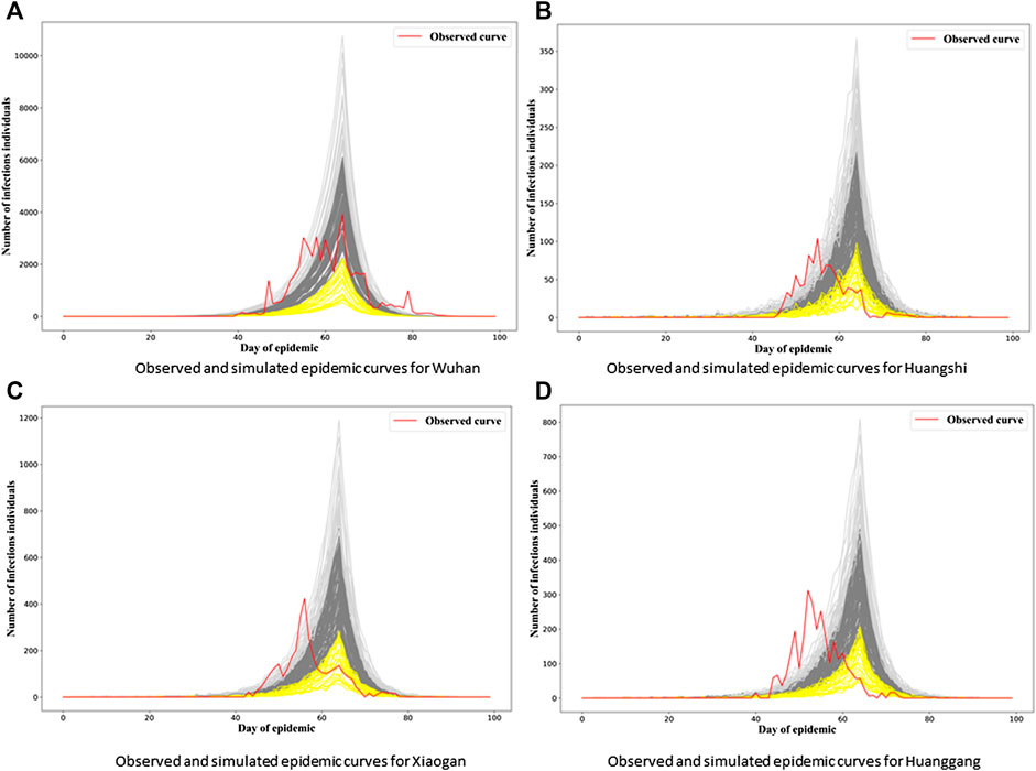
FIGURE 2. Observed and simulated epidemic curves under final model for four cities in Hubei. Real data shown in red; light gray and yellow curves represent 15% strongest and weakest epidemics simulated from the final model, respectively; remaining dark gray curves represent remaining 70% of simulated epidemics.

Of course, our model is relatively simple, assuming homogeneity between cities in terms of both the transmission process (after accounting for population dynamics) and the observation model. Our suspicion is that the observation model may be a major issue here. For example, note that the delay mechanism is mimicking both a biological process (the incubation period of the disease) and a bureaucratic process (diagnosis and processing and publication of numbers of cases per day). It therefore seems perfectly plausible that the delay between infection and reporting of cases could differ between different jurisdictions, in this case, cities.

Since the epidemic observed in Wuhan was by far the most substantial, it makes sense that the Wuhan data would be driving the inference process for the final model. It therefore makes sense that the model ends up parameterized in such a way that the data in Wuhan are mimicked well by the fitted model, and the other cities less so. Also, since Wuhan was the first city infected, it also makes sense that the delay between infection and reporting would be larger for that city and others, since it was operating with less information than other cities which had to deal with their infections a little later on.

In Figure 3, we see the “gray epidemic curves” (the 70% closest to the observed epidemic) for Wuhan. Figures 4, 5 show these “gray curves” for other cities. We can see that in Huangshi in Figure 4A, if we shift the epidemic curve based on the observed cases (shown in red) by a few days (shown in blue), the epidemic curves produced by the fitted model much better match the observed curve. Throughout Figures 4–6, we see a similar pattern for the other cities in the province.

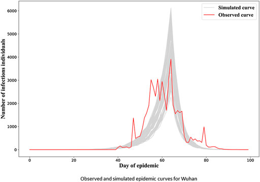
FIGURE 3. Observed and simulated epidemic curves under final model for Wuhan. Real data shown in red; dark gray curves represent 70% of curves simulated from the final model closest to the true curve.

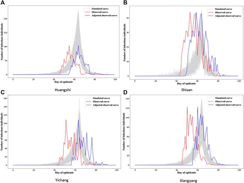
FIGURE 4. Observed and simulated epidemic curves under final model for four cities in Hubei (other 12 cities in Figures 5, 6; for Wuhan, see Figure 3). Real data shown in red; shifted real data accounting for potential differences in delays to reporting in different cities shown in blue; dark gray curves represent 70% of curves simulated from the final model closest to the true curve.

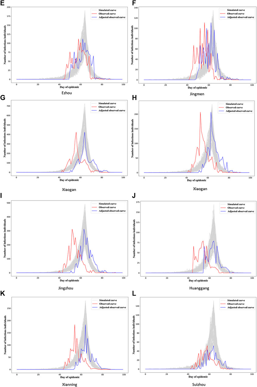
FIGURE 5. Observed and simulated epidemic curves under final model for eight cities in Hubei (other four cities in Figure 6; for Wuhan, see Figure 3). Real data shown in red; shifted real data accounting for potential differences in delays to reporting in different cities shown in blue; dark gray curves represent 70% of curves simulated from the final model closest to the true curve.

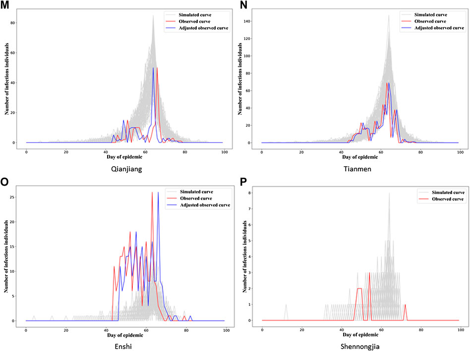
FIGURE 6. Observed and simulated epidemic curves under final model for four cities in Hubei (for Wuhan, see Figure 3). Real data shown in red; shifted real data accounting for potential differences in delays to reporting in different cities shown in blue; dark gray curves represent 70% of curves simulated from the final model closest to the true curve.

This would imply that the next step we might want to take in refining our model is to allow for heterogeneity in the observation model parameters between cities, probably starting with the delay mechanism rate parameter, $p^D$.

Overall, these results show that the two-level ILM model fitted using an ensemble classifier can reasonably well reflect the spread of SARS-CoV-2 among cities; this is especially true for Wuhan, and we can see the potential for better capturing the dynamics of COVID-19 transmission among other cities through further model development.

Conclusion

We construct a statistical inference framework that allows us to fit a two-level individual-level epidemic model to data. We use several ensemble learning classifiers to successfully estimate model parameters, avoiding the high computation costs exhibited by traditional methods of inference. The simulation study shows good performance of the fitted model, and we successfully fit our model to real data on COVID-19 transmission among 17 cities in Hubei province, China.

Future Work

In this study, we focus on analyzing the transmission of SARS-CoV-2 among 17 cities in Hubei province, China. It would certainly be of interest to see how our model performs on COVID-19 data from different countries and indeed data on other diseases. Here, also we choose to model disease transmission within an SIR framework. In many scenarios, more complex compartmental frameworks such as SEIR or SIRS would be more appropriate. It would therefore be desirable to test if classification-based inference for our model works similarly well, as well as considering such frameworks for COVID-19 transmission itself. An additional limiting factor was that we made the simplifying assumption that the infectious period was the same for all individuals. This is obviously not true in practice, and so it would be desirable to relax this assumption. There are also likely other risk factors, in addition to population size/density, we might want to include within models of COVID-19 spread to improve them. These could include demographic descriptors of age distribution within cities, knowledge about traffic flows between cities, and socioeconomic covariates.

As discussed previously, we might well wish to allow the parameters of the observation model to vary between cities, to allow for differences in recording and reporting procedures. In addition, we may want to think about allowing these parameters to change over time in line with jurisdictional government policy.

Finally, we will explore more classification methods, such as deep learning methods, to attempt to build even more accurate classifiers, especially for more complex models and populations structures.

Data Availability Statement

The original contributions presented in the study are included in the article/Supplementary Material, further inquiries can be directed to the corresponding author.

Author Contributions

ZL and RD designed and managed the project, ZL, YF, TF, and RD conceived and designed the experiments, ZL, YF, and QC analyzed the data, ZL, RD, TW, and QC wrote the manuscript.

Funding

This study is supported by the National Natural Science Foundation of China (82041020, 91846301), Natural Science Foundation of Hunan Province (2020JJ5678), and China Postdoctoral Science Foundation (2019M653922). ZL is supported by the Graduate Research and Innovation Projects of Hunan Province (CX20200069).

Conflict of Interest

The authors declare that the research was conducted in the absence of any commercial or financial relationships that could be construed as a potential conflict of interest.

Acknowledgments

ZL is supported by the CSC Scholarship offered by the China Scholarship Council.

Supplementary Material

The Supplementary Material for this article can be found online at: https://www.frontiersin.org/articles/10.3389/fphy.2020.602722/full#supplementary-material.

References

1. Fauci AS, Lane HC, Redfield RR. Covid-19—navigating the uncharted. N Engl J Med (2020) 382:1268–9. doi:10.1056/NEJMe2002387
3. Dong E, Du H, Gardner L. An interactive web-based dashboard to track COVID-19 in real time. Lancet Infect Dis (2020) 20(5):533–4. doi:10.1016/S1473-3099(20)30120-1
4. Cheng Q, Liu Z, Cheng G, Huang J. Heterogeneity and effectiveness analysis of COVID-19 prevention and control in major cities in China through time-varying reproduction numbers estimation (2020). Research Square [Preprint]. Available at: https://www.researchsquare.com/article/rs-20987/v1 (Accessed April 2, 2020).
5. Deardon R, Brooks SP, Grenfell BT, Keeling MJ, Tildesley MJ, Savill NJ, et al. Inference for individual-level models of infectious diseases in large populations. Stat Sin (2010) 20(1):239–61.
6. Anderson RM, Anderson B, May RM. Infectious diseases of humans: dynamics and control. Oxford University Press (1991) 122. p.
7. Gibson GJ. Markov chain Monte Carlo methods for fitting spatiotemporal stochastic models in plant epidemiology. J Roy Stat Soc: Series C (Applied Statistics) (1997) 46(2):215–33.
8. Keeling MJ, Woolhouse ME, Shaw DJ, Matthews L, Chase-Topping M, Haydon DT, et al. Dynamics of the 2001 UK foot and mouth epidemic: stochastic dispersal in a heterogeneous landscape. Science (2001) 294(5543):813–7. doi:10.1126/science.1065973
9. Neal PJ, Roberts GO. Statistical inference and model selection for the 1861 Hagelloch measles epidemic. Biostatistics (2004) 5(2):249–61. doi:10.1093/biostatistics/5.2.249
10. Nsoesie EO, Beckman R, Marathe M, Lewis B. Prediction of an epidemic curve: a supervised classification approach. Stat Commun Infect Dis (2011) 3(1):5. doi:10.2202/1948-4690.1038
11. Pokharel G, Deardon R. Supervised learning and prediction of spatial epidemics. Spat Spatiotemporal Epidemiol (2014) 11:59–77. doi:10.1016/j.sste.2014.08.003
12. Augusta C, Deardon R, Taylor G. Deep learning for supervised classification of spatial epidemics. Spat Spatiotemporal Epidemiol (2019) 29:187–98. doi:10.1016/j.sste.2018.08.002
13. Ferdous T. On the effect of ignoring within-unit infectious disease dynamics when modelling spatial transmission. [Master’s thesis]. Calgary (AB): University of Calgary (2019).
15. Ho TK. Random decision forests. In: Proceedings of 3rd international conference on document analysis and recognition; 1995 August 14–16; Syndey, Australia. IEEE (1995). p. 278–82.
16. Amit Y, Geman D. Shape quantization and recognition with randomized trees. Neural Comput (1997) 9(7):1545–88.
17. Friedman JH. Greedy function approximation: a gradient boosting machine. Ann Stat (2001) 1189–232.
19. Li P. Robust logitboost and adaptive base class (abc) logitboost. arXiv [Preprint] (2012). Available at: https://arxiv.org/abs/1203.3491 (Accessed March 15, 2012).
20. Chen T, Guestrin C. Xgboost: a scalable tree boosting system. In: Proceedings of the 22nd acm sigkdd international conference on knowledge discovery and data mining; San Francisco, CA; August 13–17, 2016 (2016). p. 785–94.
21. Ke G, Meng Q, Finley T, Wang T, Chen W, Ma W, et al. Lightgbm: a highly efficient gradient boosting decision tree. Adv Neural Inf Process Syst (2017). p. 3146–54.
22. Prokhorenkova L, Gusev G, Vorobev A, Dorogush AV, Gulin A. CatBoost: unbiased boosting with categorical features. Adv Neural Inf Process Syst (2018). p. 6638–48.
Keywords: COVID-19 epidemic, individual-level model, SARS-CoV-2 transmission, spatiotemporal analysis, ensemble learning classifiers
Citation: Liu Z, Deardon R, Fu Y, Ferdous T, Ware T and Cheng Q (2021) Estimating Parameters of Two-Level Individual-Level Models of the COVID-19 Epidemic Using Ensemble Learning Classifiers. Front. Phys. 8:602722. doi: 10.3389/fphy.2020.602722
Received: 04 September 2020; Accepted: 12 November 2020;
Published: 21 January 2021.
Edited by:
Hui-Jia Li, Beijing University of Posts and Telecommunications (BUPT), ChinaReviewed by:
Qianqian Tong, University of Connecticut, United StatesYanmi Wu, Zhengzhou University, China
Copyright © 2021 Liu, Deardon, Fu, Ferdous, Ware and Cheng. This is an open-access article distributed under the terms of the Creative Commons Attribution License (CC BY). The use, distribution or reproduction in other forums is permitted, provided the original author(s) and the copyright owner(s) are credited and that the original publication in this journal is cited, in accordance with accepted academic practice. No use, distribution or reproduction is permitted which does not comply with these terms.
*Correspondence: Qing Cheng, sgggps@163.com