Perturbative Approach to Effective Shell-Model Hamiltonians and Operators

Coraggio, Luigi; Itaco, Nunzio

doi:10.3389/fphy.2020.00345

REVIEW article

Front. Phys., 15 October 2020
Sec. Nuclear Physics
Volume 8 - 2020 | https://doi.org/10.3389/fphy.2020.00345

Perturbative Approach to Effective Shell-Model Hamiltonians and Operators

Luigi Coraggio¹^*

Nunzio Itaco^1,2^*

¹Istituto Nazionale di Fisica Nucleare, Sezione di Napoli, Naples, Italy
²Dipartimento di Matematica e Fisica, Università degli Studi della Campania “Luigi Vanvitelli”, Caserta, Italy

This article presents an overview of the derivation of effective shell-model Hamiltonian and decay operators within the framework of many-body perturbation theory, and discusses the results of selected shell-model studies based on these operators. More precisely, we give technical details that non-experts will need in order to derive shell-model Hamiltonians and operators starting from realistic nuclear potentials, and provide some guidance for shell-model calculations where the single-particle energies, two-body matrix elements of the residual interaction, effective charges, and decay matrix elements are all obtained without resorting to empirical adjustments. We report results of studies of double-β decay of heavy-mass nuclei where the shell-model ingredients are derived from theory, so as to assess the reliability of such an approach to shell-model investigations. Attention will be also focused on aspects relating to the behavior of the perturbative expansion, knowledge of which is needed for establishing limits and applying this approach to nuclear structure calculations.

1. Introduction

This article presents formal details of the derivation of effective shell-model Hamiltonians (H_eff) and decay operators by a perturbative approach, and reviews a large sample of recent applications to the study of spectroscopic properties of atomic nuclei. The goal of this work is to provide a useful tool for practitioners who are interested in using shell-model single-particle energies, two-body matrix elements, effective charges, and magnetic-dipole and β-decay operators, which are derived from many-body theory, to reproduce a selection of observables without resorting to parameters that are empirically adjusted.

The well-known nuclear shell model (SM) is widely considered a basic theoretical tool for the microscopic description of nuclear structure properties. The nuclear SM is based on the ansatz that each nucleon inside the nucleus moves independently of other nucleons, in a spherically symmetric mean field plus a strong spin-orbit term. This first-approximation depiction of a nucleus is supported by the observation of “magic numbers” of protons and/or neutrons, corresponding to nuclei which are more tightly bound than their neighbors.

These considerations have led to depictions of nucleons arranging themselves into groups of energy levels, called “shells,” that are well-separated from each other. The main result of the SM scheme is the reduction of the complex nuclear many-body problem to a very simplified setting where only a few valence nucleons interact in a reduced model space spanned by a single major shell situated above an inert core.

The cost of such a simplification is that shell-model wave functions, which describe the independent motions of individual nucleons, do not include the correlations induced by the strong short-range bare interaction, and therefore could be very different from the real wave functions of the nuclei. The SM Hamiltonian, which will be introduced in the next section, contains one- and two-body components whose characterizing parameters, namely the single-particle (SP) energies and two-body matrix elements (TBMEs) of the residual interaction, account for the degrees of freedom that are not explicitly included in the truncated Hilbert space of the configurations. As a matter of fact, SP energies and TBMEs should be determined to include, in an effective way, the excitations of both the core nucleons and the valence nucleons in the shells above the model space.

Derivation of the effective SM Hamiltonian may follow two distinct paths. One approach is phenomenological: that is, the one- and two-body components of the Hamiltonian are adjusted to reproduce a selected set of experimental data. This can be done either by using an analytical expression for the residual interaction with adjustable parameters, or by treating the Hamiltonian matrix elements directly as free parameters (see [1, 2]).

Over more than 70 years of SM calculations, this approach has been very successful at reproducing a huge amount of data and describing some of the most fundamental physical properties of the structure of atomic nuclei. In this regard, it is worth mentioning the review by Caurier et al. [3], which contains an interesting discussion about the properties of the effective SM Hamiltonian; additional references will be given in the following section.

Another way of constructing H_eff is to start from realistic nuclear forces—two- and three-body potentials if possible—and derive the effective Hamiltonian in the framework of many-body theory, i.e., obtain an H_eff whose eigenvalues belong to the set of eigenvalues of the full nuclear Hamiltonian defined in the whole Hilbert space.

To do this, one needs a similarity transformation which, within the full Hilbert space of the configurations, leads to a decoupling of the model space P, where the valence nucleons are constrained, from its complement Q = 1 − P. Nowadays this can be achieved within the framework of ab initio methods, which aim to solve the full Hamiltonian of A nucleons by employing controlled truncations of the accessible degrees of freedom. However, this approach is strictly limited by the computational power available and, even if successful, is currently confined to just a few nuclear mass regions. A comprehensive survey of possible ways to tackle the problem of deriving H_eff starting from ab initio methods can be found in reference [4], where some SM applications and results are also reviewed.

The present work focuses on perturbative expansion of the effective SM Hamiltonian, grounded in the energy-independent linked-diagram perturbation theory [5], which has been extensively used in SM calculations over the past 50 years (see also the review papers [6, 7]).

An earlier attempt along this line was made by Bertsch [8], who employed as interaction vertices the matrix elements of the reaction matrix G derived from the Kallio-Kolltveit potential [9] to study the role played by the core-polarization diagram at second order in perturbation theory, accounting for one-particle-one-hole (1p-1h) excitations above the Fermi level of the core nucleons. The results of this work showed that the contribution of such a diagram to H_eff was about 30% of the first-order two-body matrix element, when considering the open-shell nuclei ¹⁸O and ⁴²Sc outside doubly closed cores ¹⁶O and ⁴⁰Ca, respectively.

Then came the seminal paper by Tom Kuo and Gerry Brown [10], which represents a true turning point in nuclear structure theory. It includes the first successful attempt at performing a shell-model calculation starting from the free nucleon-nucleon (NN) Hamada-Johnston (HJ) potential [11], and resulted in a quantitative description of the spectroscopic properties of sd-shell nuclei.

The TBMEs of the sd-shell effective interaction in reference [10] were derived starting from the HJ potential, with the hard-core component renormalized via calculation of the reaction matrix G. The matrix elements of G were then used as interaction vertices in the perturbative expansion of H_eff, including terms up to second order in G.

The TBMEs obtained by this approach were used to calculate the energy spectra of ¹⁸O and ¹⁸F and yielded results in good agreement with experiments. Moreover, these matrix elements, as well as those derived 2 years later for SM calculations in the fp-shell [12], have become the backbone of the fine-tuning of successful empirical SM Hamiltonians, such as the USD [13] and the KB3G potentials [3, 14].

Between the late 1960s and early 1970s the theoretical framework evolved thanks to the introduction of the folded-diagrams expansion, which formally defined the correct procedure for the perturbative expansion of effective SM Hamiltonians [15, 16].

In the forthcoming sections we will present in detail the derivation of H_eff and consistent effective SM decay operators, within the theoretical framework of many-body perturbation theory. At the core of our approach is the perturbative expansion of two vertex functions, the so-called $\hat{Q}$ -box and $\hat{Θ}$ -box, in terms of irreducible valence-linked Goldstone diagrams. The $\hat{Q}$ -box is then employed to solve non-linear matrix equations in order to obtain H_eff by way of iterative techniques [17], and the latter together with the $\hat{Θ}$ -box are the main ingredients for deriving the effective decay operators [18].

This paper is organized as follows. In the next section we present a general overview of the SM eigenvalue problem and the derivation of the effective SM Hamiltonian. In section 3 we tackle the problem on the basis of the Lee-Suzuki similarity transformation [17, 19] and introduce the iterative procedures for solving the decoupling equation that provides this similarity transformation into H_eff, for both degenerate and non-degenerate model spaces. Two subsections are devoted to the perturbative expansion of the $\hat{Q}$ -box vertex function and the derivation of effective SM decay operators. In section 4 we summarize results of investigations into the double-β decay of ¹³⁰Te and ¹³⁶Xe, and discuss the perturbative properties of H_eff and effective SM decay operators. The final section gives a summary of the present work.

2. General Overview

As mentioned in the Introduction, the SM, introduced 70 years ago [20, 21], is based on the assumption that, as a first approximation, each nucleon (proton or neutron) inside the nucleus moves independently in a spherically symmetric potential representing the average interaction with the other nucleons. This potential is usually described by a Woods-Saxon or harmonic oscillator potential plus a strong spin-orbit term. Inclusion of the latter term is crucial to producing single-particle states clustered in groups of orbits that are close in energy (shells). Each shell is well-separated in energy from the other shells, and this enables the nucleus to be schematized as an inert core, made up of shells filled with neutrons and protons paired to give a total angular momentum of J = 0⁺, plus a certain number of external nucleons, the so-called “valence” nucleons. This extreme single-particle SM is able to successfully describe various nuclear properties [22], such as the angular momentum and parity of the ground states in odd-mass nuclei. However, it is clear that in order to describe the low-energy structure of nuclei with two or more valence nucleons, the “residual” interaction between the valence nucleons has to be considered explicitly, where the term “residual” refers to that part of the interaction which is not taken into account by the central potential. The inclusion of the residual interaction removes the degeneracy of states belonging to the same configuration and produces a mixing of different configurations.

Let us now use the simple nucleus ¹⁸O to introduce some common terminology used in effective interaction theories.

Suppose we want to calculate the properties of the low-lying states in ¹⁸O. Then we must solve the Schrödinger equation

\begin{array}{l} H | Ψ_{ν} 〉 = E_{ν} | Ψ_{ν} 〉, & (1) \end{array}

where

\begin{array}{l} H = H_{0} + H_{1} & (2) \end{array}

with

\begin{array}{l} H_{0} = \sum_{i = 1}^{A} (\frac{p_{i}^{2}}{2 m} + U_{i}) & (3) \end{array}

and

\begin{array}{l} H_{1} = \sum_{i < j = 1}^{A} V_{i j}^{N N} - \sum_{i = 1}^{A} U_{i} . & (4) \end{array}

An auxiliary one-body potential U_i has been introduced to decompose the nuclear Hamiltonian as the sum of a one-body term H₀, which describes the independent motion of the nucleons, and the residual interaction H₁. It is worth pointing out that in the following, for the sake of simplicity and without any loss of generality, we will assume that the interaction between the nucleons is described by a two-body force only, neglecting three-body contributions. The generalization of the formalism to include three-nucleon forces may be found in references [23, 24].

It is customary to choose an auxiliary one-body potential U of convenient mathematical form, such as the harmonic oscillator potential

\begin{array}{l} U = \sum_{i = 1}^{A} \frac{1}{2} m ω r_{i}^{2} . & (5) \end{array}

In Figure 1 we show the relevant portion of the H₀ spectrum for ¹⁸O.

FIGURE 1

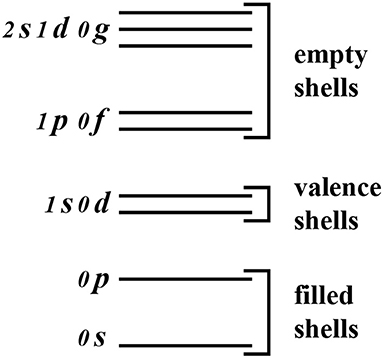
Figure 1. Energy shells that characterize the core, valence space, and empty orbitals for ¹⁸O.

We expect the wave functions of the low-lying states in ¹⁸O to be dominated by components with a closed ¹⁶O core (i.e., the 0s and 0p orbits are filled) and two neutrons in the valence orbits 1s and 0d. Hence, we choose a model space spanned by the vectors

\begin{array}{l} | Φ_{i} 〉 = \sum_{α, β \in valence space} C_{α β}^{i} {[a_{α}^{†} a_{β}^{†}]}_{i} | c 〉, i = 1, \dots, d, & (6) \end{array}

where |c〉 represents the unperturbed ¹⁶O core obtained by completely filling the 0s and 0p orbits,

\begin{array}{l} | c 〉 = \prod_{α \in filled shells} a_{α}^{†} | 0 〉, & (7) \end{array}

and the index i stands for all the other quantum numbers needed to specify the state (e.g., the total angular momentum).

To illustrate the situation, we show in Figure 2 some SM configurations labeled in terms of particles and holes with respect to the ¹⁶O core.

FIGURE 2

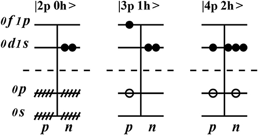
Figure 2. Some ¹⁸O shell-model configurations.

Solving Equation (1) using basis vectors like those shown in Figure 2 amounts to diagonalizing the infinite matrix H in Figure 3. This is infeasible, so we seek to reduce this huge matrix to a smaller one, H_eff, with the requirement that the eigenvalues of the latter should belong to the set of eigenvalues of the former. The notation |2p′ 0h〉 represents a configuration with a closed ¹⁶O core plus two particles constrained to interact in the sd-shell.

FIGURE 3

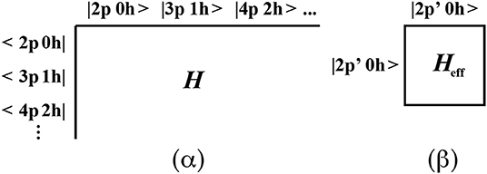
Figure 3. Representation of the matrices H and H_eff for ¹⁸O.

More formally, it is convenient to define the projection operators P and Q = 1 − P, which project from the complete Hilbert space onto the model space and its complementary space (excluded space), respectively. The operator P can be expressed in terms of the vectors in Equation (6) as

\begin{array}{l} P = \sum_{i = 1}^{d} | Φ_{i} 〉 〈 Φ_{i} | . & (8) \end{array}

The projection operators P and Q satisfy the properties

\begin{array}{l} P^{2} = P, Q^{2} = Q, P Q = Q P = 0 . & (9) \end{array}

The key idea of the effective SM interaction theory is to transform the eigenvalue problem of Equation (1) into a reduced model-space eigenvalue problem

\begin{array}{l} P H_{eff} P | Ψ_{α} 〉 = (E_{α} - E_{C}) P | Ψ_{α} 〉, & (10) \end{array}

where E_C is the true energy of the core, i.e., the true ground-state energy of ¹⁶O in the present case.

As mentioned in the Introduction, there are two main approaches to deriving H_eff:

• a phenomenological approach;

• an approach that starts from the bare nuclear interactions and makes use of an appropriate many-body theory.

In the phenomenological approach, empirical effective interactions containing adjustable parameters are introduced and modified to fit a certain set of experimental data, or the two-body matrix elements themselves are treated as free parameters. This approach has been very successful, and we refer to several excellent reviews [2, 3, 25–27] for a comprehensive discussion of the topic.

Currently there are several ways to derive an effective SM Hamiltonian starting from the bare interactions between nucleons. In fact, besides the well-established approaches based on many-body perturbation theory [5] or the Lee-Suzuki transformation [17, 19], novel non-perturbative methods, such as valence-space in-medium similarity renormalization group (VS-IMSRG) [28], shell-model coupled cluster (SMCC) [29], or the no-core shell model (NCSM) with a core based on the Lee-Suzuki similarity transformation [30–33], are now available. These non-perturbative approaches are firmly rooted in many-body theory and provide somewhat different paths to H_eff. They can be derived in the same general theoretical framework by expressing H_eff as the result of a similarity transformation acting on the original Hamiltonian,

\begin{array}{l} H_{eff} = e^{G} H e^{- G}, & (11) \end{array}

where the transformation is parameterized as the exponential of a generator $G$ , such that the decoupling condition

\begin{array}{l} Q H_{eff} P = 0 & (12) \end{array}

is satisfied. Reference [4] contains a very detailed discussion of how the different methods (perturbative and non-perturbative) can be derived within such a general framework, as well as descriptions of the corresponding approximation schemes employed in each approach.

As stated in the Introduction, the present review aims to describe in detail the perturbative approach to the derivation of H_eff; this is the focus of the next section. We refer to the already cited review paper by Stroberg et al. [4] for an exhaustive description of alternative methods.

3. Perturbative Expansion of Effective Shell-Model Operators

3.1. The Lee-Suzuki Similarity Transformation

In this subsection we present the formalism of the derivation of the effective SM Hamiltonian based on the similarity transformation introduced by Lee and Suzuki [19]. It is worth noting that this approach has been very successful since it makes a straightforward perturbative expansion of H_eff possible for open-shell systems outside a closed core, whereas in other approaches, such as the oscillator-based effective theory (HOBET) proposed by Haxton and Song [34] or the coupled-cluster similarity transformation [35], factorization of the core configurations with respect to the valence nucleons is far more complicated to perform.

We start from the Schrödinger equation for the A-nucleon system, defined in the whole Hilbert space:

\begin{array}{l} H | Ψ_{ν} 〉 = E_{ν} | Ψ_{ν} 〉 . & (13) \end{array}

As already mentioned, within the SM framework an auxiliary one-body potential U is introduced to express the nuclear Hamiltonian as the sum of an unperturbed one-body mean-field term H₀ and the residual interaction Hamiltonian H₁. The full Hamiltonian H is then rewritten in terms of H₀ and H₁, as in Equations (2)–(4).

According to the nuclear SM described in the previous section, the nucleus may be thought of as a frozen core, composed of a number of nucleons which fill a certain number of energy shells generated by the spectrum of the one-body Hamiltonian H₀, plus a remainder of n interacting valence nucleons moving in the mean field H₀.

The large energy gap between the shells allows us to regard the A − n core nucleons, which completely fill the shells that are lowest in energy, as inert. The SP states accessible to the valence nucleons are those belonging to the major shell situated (in energy) just above the closed core. The configurations allowed by the valence nucleons within this major shell define a reduced Hilbert space, the model space, in terms of a finite subset of d eigenvectors of H₀, as expressed in Equation (6).

We then consider the projection operators P (see Equation 8) and Q = 1 − P, which project from the complete Hilbert space onto the model space and its complementary space, respectively, and satisfy the properties in Equation (9).

The goal of an SM calculation is to reduce the eigenvalue problem of Equation (13) to the model-space eigenvalue problem

\begin{array}{l} H_{eff} P | Ψ_{α} 〉 = E_{α} P | Ψ_{α} 〉, α = 1, \dots, d, & (14) \end{array}

where H_eff is defined only in the model space.

This means that we are looking for a new Hamiltonian $H$ whose eigenvalues are the same as those of the Hamiltonian H for the A-nucleon system but which satisfies the decoupling equation between the model space P and its complement Q:

\begin{array}{l} Q H P = 0, & (15) \end{array}

which guarantees that the desired effective Hamiltonian is $H_{eff} = P H P$ .

The Hamiltonian $H$ should be obtained by way of a similarity transformation defined in the whole Hilbert space:

\begin{array}{l} H = X^{- 1} H X . & (16) \end{array}

Of course, the class of transformation operators X that satisfy the decoupling Equation (15) is infinite, and Lee and Suzuki [17, 19] proposed an operator X defined as X = e^ω. Without loss of generality, ω can be chosen to satisfy the following properties:

\begin{array}{l} ω = Q ω P, & (17) \end{array}

\begin{array}{l} P ω P = Q ω Q = P ω Q = 0 . & (18) \end{array}

Equation (17) implies that

\begin{array}{l} ω^{2} = ω^{3} = \dots = 0 . & (19) \end{array}

According to the above equation, X may be written as X = 1 + ω, and consequently we have the following expression for H_eff:

\begin{array}{l} H_{eff} = P H P = P H P + P H Q ω . & (20) \end{array}

The operator ω may be calculated by solving the decoupling Equation (15), and the latter can be rewritten as

\begin{array}{l} Q H P + Q H Q ω - ω P H P - ω P H Q ω = 0 . & (21) \end{array}

This matrix equation is non-linear, and once the Hamiltonian H is expressed explicitly in the whole Hilbert space, it can be easily solved. Actually, this is not an easy task for nuclei with mass A > 2, and, as mentioned in the previous section, this approach has been employed only for light nuclei within the ab initio framework.

A successful way to solve Equation (21) for SM calculations is to use a vertex function, the $\hat{Q}$ -box, which is suitable for a perturbative expansion. We now explain the $\hat{Q}$ -box approach to deriving H_eff. It is important to note that in the following we assume our model space to be degenerate:

\begin{array}{l} P H_{0} P = ϵ_{0} P . & (22) \end{array}

Then, thanks to the decoupling Equation (15), the effective Hamiltonian $H_{1}^{eff} = H_{eff} - P H_{0} P$ can be expressed as a function of ω:

\begin{array}{l} H_{1}^{eff} = P H P - P H_{0} P = P H_{1} P + P H_{1} Q ω . & (23) \end{array}

The above identity, the decoupling Equation (21), and the properties of H₀ and H₁ allow us to define recursively the effective Hamiltonian $H_{1}^{eff}$ . First, since H₀ is diagonal, we can write the following identity:

\begin{array}{l} Q H P = Q H_{1} P + Q H_{0} P = Q H_{1} P . & (24) \end{array}

Then, the decoupling Equation (21) can be rewritten in the form

\begin{array}{l} Q H_{1} P + Q H Q ω - ω (P H_{0} P + P H_{1} P + P H_{1} Q ω) \\ = Q H_{1} P + Q H Q ω - ω (ϵ_{0} P + H_{1}^{eff}) = 0 . & (25) \end{array}

Using this expression for the decoupling equation, we can write a new identity for the operator ω:

\begin{array}{l} ω = Q \frac{1}{ϵ_{0} - Q H Q} Q H_{1} P - Q \frac{1}{ϵ_{0} - Q H Q} ω H_{1}^{eff} . & (26) \end{array}

Finally, we obtain a recursive equation by substituting Equation (26) into the identity (23):

\begin{array}{l} H_{1}^{eff} (ω) = P H_{1} P + P H_{1} Q \frac{1}{ϵ_{0} - Q H Q} Q H_{1} P \\ - P H_{1} Q \frac{1}{ϵ_{0} - Q H Q} ω H_{1}^{eff} (ω) . & (27) \end{array}

We now define the $\hat{Q}$ -box vertex function as

\begin{array}{l} \hat{Q} (ϵ) = P H_{1} P + P H_{1} Q \frac{1}{ϵ - Q H Q} Q H_{1} P, & (28) \end{array}

and this allows us to express the recursive Equation (27) as

\begin{array}{l} H_{1}^{eff} (ω) = \hat{Q} (ϵ_{0}) - P H_{1} Q \frac{1}{ϵ_{0} - Q H Q} ω H_{1}^{eff} (ω) . & (29) \end{array}

As can be seen from both of the Equations (28) and (29), configurations belonging to the Q space that have energy close to the unperturbed energy of model-space configurations (intruder states) may give unstable solutions of Equation (29). This is the so-called “intruder-state problem” as pointed out in references [36, 37] by Schucan and Weidenmüller. In the following we first present two possible iterative techniques for solving Equation (29), as suggested by Lee and Suzuki [17]. These methods, which are based on calculation of the $\hat{Q}$ -box and its derivatives, are known as the Krenciglowa-Kuo and Lee-Suzuki techniques. In particular, we point out that in reference [17] it is shown that the Lee-Suzuki iterative procedure is convergent even when there are some intruder states. We will then present some other approaches that generalize the derivation of H_eff, based on calculation of the $\hat{Q}$ -box, to unperturbed Hamiltonians H₀ which provide non-degenerate model spaces.

3.1.1. The Krenciglowa-Kuo Iterative Technique

The Krenciglowa-Kuo (KK) iterative technique for solving the recursive Equation (29) is based on the coupling of Equations (29) and (26), which gives the iterative equation

\begin{array}{l} H_{1}^{eff} (ω_{n}) = \sum_{m = 0}^{\infty} [- P H_{1} Q {(\frac{- 1}{ϵ_{0} - Q H Q})}^{m + 1} Q H_{1} P] \\ {[H_{1}^{eff} (ω_{n - 1})]}^{m} . & (30) \end{array}

The quantity inside the first set of square brackets in Equation (30), which will be denoted by ${\hat{Q}}_{m} (ϵ_{0})$ from now on, is proportional to the mth derivative of the $\hat{Q}$ -box calculated at ϵ = ϵ₀:

\begin{array}{l} {\hat{Q}}_{m} (ϵ_{0}) = - P H_{1} Q {(\frac{- 1}{ϵ_{0} - Q H Q})}^{m + 1} \\ Q H_{1} P = \frac{1}{m!} {[\frac{d^{m} \hat{Q} (ϵ)}{d ϵ^{m}}]}_{ϵ = ϵ_{0}} . & (31) \end{array}

We may then rewrite Equation (30) according to the above identity as

\begin{array}{l} H_{1}^{eff} (ω_{n}) = \sum_{m = 0}^{\infty} \frac{1}{m!} {[\frac{d^{m} \hat{Q} (ϵ)}{d ϵ^{m}}]}_{ϵ = ϵ_{0}} \\ {[H_{1}^{eff} (ω_{n - 1})]}^{m} = \sum_{m = 0}^{\infty} {\hat{Q}}_{m} (ϵ_{0}) {[H_{1}^{eff} (ω_{n - 1})]}^{m} . & (32) \end{array}

The starting point of the KK iterative method is the assumption that $H_{1}^{eff} (ω_{0}) = \hat{Q} (ϵ_{0})$ , which enables us to rewrite Equation (32) in the form

\begin{array}{l} H^{eff} = \sum_{i = 0}^{\infty} F_{i}, & (33) \end{array}

where

\begin{array}{l} F_{0} = \hat{Q} (ϵ_{0}), \\ F_{1} = {\hat{Q}}_{1} (ϵ_{0}) \hat{Q} (ϵ_{0}), \\ F_{2} = {\hat{Q}}_{2} (ϵ_{0}) \hat{Q} (ϵ_{0}) \hat{Q} (ϵ_{0}) + {\hat{Q}}_{1} (ϵ_{0}) {\hat{Q}}_{1} (ϵ_{0}) \hat{Q} (ϵ_{0}), \\ ⋮ & (34) \end{array}

Expression (33) is the well-known folded-diagram expansion of the effective Hamiltonian introduced by Kuo and Krenciglowa. In reference [38] they demonstrated the following operatorial identity:

\begin{array}{l} {\hat{Q}}_{1} \hat{Q} = - \hat{Q} \int \hat{Q}, & (35) \end{array}

where the integral sign corresponds to the so-called folding operation introduced by Brandow in reference [15].

3.1.2. The Lee-Suzuki Iterative Technique

The Lee-Suzuki (LS) technique is another iterative procedure, which is carried out by rearranging Equation (29) to obtain an explicit expression for the effective Hamiltonian $H_{1}^{eff}$ in terms of the operators ω and $\hat{Q}$ [17]:

\begin{array}{l} H_{1}^{eff} (ω) = {(1 + P H_{1} Q \frac{1}{ϵ_{0} - Q H Q} ω)}^{- 1} \hat{Q} (ϵ_{0}) . & (36) \end{array}

The iterative form of the above equation is

\begin{array}{l} H_{1}^{eff} (ω_{n}) = {(1 + P H_{1} Q \frac{1}{ϵ_{0} - Q H Q} ω_{n - 1})}^{- 1} \hat{Q} (ϵ_{0}), & (37) \end{array}

and we may also write an iterative expression for Equation (26):

\begin{array}{l} ω_{n} = Q \frac{1}{ϵ_{0} - Q H Q} Q H_{1} P - Q \frac{1}{ϵ_{0} - Q H Q} ω_{n - 1} H_{1}^{eff} (ω_{n}) . & (38) \end{array}

The standard procedure is to start the iteration by choosing ω₀ = 0, so that we may write

\begin{array}{l} H_{1}^{eff} (ω_{1}) = \hat{Q} (ϵ_{0}), \\ ω_{1} = Q \frac{1}{ϵ_{0} - Q H Q} Q H_{1} P . \end{array}

After some algebra, the following identity can be established:

\begin{array}{l} {\hat{Q}}_{1} (ϵ_{0}) = - P H_{1} Q \frac{1}{ϵ_{0} - Q H Q} Q \frac{1}{ϵ_{0} - Q H Q} \\ Q H_{1} P = - P H_{1} Q \frac{1}{ϵ_{0} - Q H Q} ω_{1} . & (39) \end{array}

Then for the n = 2 iteration we have

\begin{array}{l} H_{1}^{eff} (ω_{2}) = {(1 + P H_{1} \frac{1}{ϵ_{0} - Q H Q} ω_{1})}^{- 1} \hat{Q} (ϵ_{0}) \\ = \frac{1}{1 - {\hat{Q}}_{1} (ϵ_{0})} \hat{Q} (ϵ_{0}), \\ ω_{2} = Q \frac{1}{ϵ_{0} - Q H Q} Q H_{1} P - Q \frac{1}{ϵ_{0} - Q H Q} ω_{1} H_{1}^{eff} (ω_{2}) . & (40) \end{array}

Finally, the LS iterative expression for H_eff is

\begin{array}{l} H_{1}^{eff} (ω_{n}) = {[1 - {\hat{Q}}_{1} (ϵ_{0}) \sum_{m = 2}^{n - 1} {\hat{Q}}_{m} (ϵ_{0}) \prod_{k = n - m + 1}^{n - 1} H_{1}^{eff} (ω_{k})]}^{- 1} \hat{Q} (ϵ_{0}) . & (41) \end{array}

It is important to realize that the KK and LS iterative techniques, which allow the solution of the decoupling Equation (25), do not in principle provide the same H_eff. Suzuki and Lee have shown that the KK iterative approach provides an effective Hamiltonian whose eigenstates have the largest overlap with the eigenstates of the model space, and that H_eff obtained from the LS technique has eigenvalues that are lowest in energy among those belonging to the set of the full Hamiltonian H [17].

Both the KK and the LS procedures are limited to employing an unperturbed Hamiltonian H₀ whose model-space eigenstates are degenerate in energy. However, reference [39] introduced an alternative approach to the KK and LS techniques, which extends these methods to the case of non-degenerate H₀ by using multi-energy $\hat{Q}$ -boxes. This approach is quite involved in practice, and the only existing application in the literature is that in reference [40].

We next outline two methods [41, 42] for deriving effective SM Hamiltonians which may be implemented straightforwardly with H₀'s that are non-degenerate in the model space.

3.1.3. The Kuo-Krenciglowa Technique Extended to Non-degenerate Model Spaces

The extended Kuo-Krenciglowa (EKK) method is an extension of the KK iterative technique that can be used to derive an H_eff within non-degenerate model spaces [41, 43]. We summarize the EKK method as follows.

First, a shifted Hamiltonian $\tilde{H}$ is defined in terms of an energy parameter E:

\begin{array}{l} \tilde{H} = H - E . & (42) \end{array}

Then we rewrite Equation (25) in terms of $\tilde{H}$ :

\begin{array}{l} (E - Q H Q) ω = Q H_{1} P - ω P \tilde{H} P - ω P H_{1} Q ω = Q H_{1} P - ω {\tilde{H}}_{eff} . & (43) \end{array}

Equation (43) may be solved by an iterative procedure analogous to the KK technique, in terms of the $\hat{Q}$ -box and its derivatives as defined in Equations (28) and (31), respectively.

The effective Hamiltonian ${\tilde{H}}_{eff}$ at the nth step of the iterative procedure may then be expressed as [41]

\begin{array}{l} {\tilde{H}}_{eff}^{(n)} = {\tilde{H}}_{BH} (0) + \sum_{k = 1}^{\infty} {\hat{Q}}_{k} (0) {[{\tilde{H}}_{eff}^{(n - 1)}]}^{k}, & (44) \end{array}

where ${\tilde{H}}_{BH}$ is the solution of the Bloch-Horowitz equation [44]:

\begin{array}{l} {\tilde{H}}_{BH} (E) = P \tilde{H} P + P H_{1} Q \frac{1}{E - Q H Q} Q H_{1} P . & (45) \end{array}

We note that the EKK method does not require H₀ to be degenerate within the model space; it has therefore been applied to derive H_eff in a multi-shell valence space [45, 46] and in Gamow SM calculations with realistic NN potentials [47, 48].

It is worth pointing out that, since ${\tilde{H}}_{eff} = lim_{n \to \infty} {\tilde{H}}_{eff}^{(n)}$ , we can write

\begin{array}{l} {\tilde{H}}_{eff} = {\tilde{H}}_{BH} (0) + \sum_{k = 1}^{\infty} {\hat{Q}}_{k} (0) {[{\tilde{H}}_{eff}]}^{k} . & (46) \end{array}

Equation (46) may be interpreted as a Taylor series expansion of ${\tilde{H}}_{eff}$ about ${\tilde{H}}_{BH}$ , and the parameter E corresponds to a shift of the origin of the expansion and a resummation of the series [45]. In fact, by virtue of Equation (42) we may express H_eff as

\begin{array}{l} H_{eff} = {\tilde{H}}_{eff} + E = H_{BH} (0) + \sum_{k = 1}^{\infty} {\hat{Q}}_{k} (0) {[{\tilde{H}}_{eff}]}^{k} . & (47) \end{array}

Now, both sides of the above equation are independent of E provided that the summation is carried out at infinity, and the parameter E may be tuned to accelerate the convergence of the series when in practical applications a numerical partial summation needs to be employed and a perturbative expansion of the $\hat{Q}$ -box is carried out [45].

3.1.4. The $\hat{Z}$ (ϵ) Vertex Function

Suzuki and coworkers proposed in reference [42] an approach to the derivation of H_eff that aims to avoid the divergences of the $\hat{Q}$ -box vertex function when a non-degenerate model space is considered. In fact, the definition of the $\hat{Q}$ -box in Equation (28) shows that if ϵ approaches one of the eigenvalues of QHQ, then instabilities may arise if one employs a numerical derivation, since these eigenvalues are poles of $\hat{Q} (ϵ)$ .

We now sketch the procedure described in reference [42] and, for the sake of simplicity, consider the case of a degenerate unperturbed model space (i.e., PH₀P = ϵ₀P).

A new vertex function $\hat{Z}$ (ϵ) is introduced and defined in terms of $\hat{Q} (ϵ)$ and its first derivative as

\begin{array}{l} \hat{Z} (ϵ) \equiv \frac{1}{1 - {\hat{Q}}_{1} (ϵ)} [\hat{Q} (ϵ) - {\hat{Q}}_{1} (ϵ) (ϵ - ϵ_{0}) P] . & (48) \end{array}

It can be demonstrated that $\hat{Z}$ (ϵ) satisfies the equation [42]

\begin{array}{l} [ϵ_{0} + \hat{Z} (E_{α})] P | Ψ_{α} 〉 = E_{α} P | Ψ_{α} 〉, α = 1, \dots, d . & (49) \end{array}

Consequently, $H_{1}^{eff}$ may be obtained by calculating the $\hat{Z}$ -box for those values of the energy, determined self-consistently, that correspond to the “true” eigenvalues E_α.

To calculate E_α, we solve the eigenvalue problem

\begin{array}{l} [ϵ_{0} + \hat{Z} (ϵ)] | ϕ_{k} 〉 = F_{k} (ϵ) | ϕ_{k} 〉, k = 1, 2, \dots, d, & (50) \end{array}

where F_k(ϵ) are d eigenvalues that depend on ϵ. Then, the true eigenvalues E_α can be obtained by solving the d equations

\begin{array}{l} ϵ = F_{k} (ϵ), k = 1, 2, \dots, d . & (51) \end{array}

First, it is worth pointing out some fundamental properties of $\hat{Z}$ (ϵ) and the associated functions F_k(ϵ). We then proceed to discuss the solution of the Equations (50) and (51).

The behavior of $\hat{Z}$ (ϵ) near the poles of $\hat{Q} (ϵ)$ is dominated by ${\hat{Q}}_{1} (ϵ)$ , and we may write $\hat{Z}$ (ϵ) ≈ (ϵ − ϵ₀)P. This means that $\hat{Z}$ (ϵ) has no poles and so the F_k(ϵ)'s are continuous and differentiable functions for any value of ϵ.

The Equations (51) may have solutions that do not correspond to the true eigenvalues E_α, i.e., spurious solutions. In reference [42] it is shown that since the energy derivative of F_k(ϵ) approaches zero at ϵ = E_α, study of this derivative provides a criterion for locating and rejecting spurious solutions. The solution of Equations (50) and (51), which is necessary for deriving the effective interaction, may be achieved through both iterative and non-iterative methods.

We describe here a graphical non-iterative method for solving Equation (51). As mentioned before, the F_k(ϵ)'s are continuous functions of the energy, and hence the solutions of Equation (51) may be determined as intersections of the graphs y = ϵ and y = F_k(ϵ), using one of the well-known algorithms for solving non-linear equations.

More precisely, if we define the functions f_k(ϵ) as f_k(ϵ) = F_k(ϵ) − ϵ, the solutions of Equation (51) can obtained by finding the roots of the equations f_k(ϵ) = 0. From inspection of the graphs y = ϵ and y = F_k(ϵ), we can locate for each intersection a small surrounding interval [ϵ_a, ϵ_b] where f_k(ϵ_a)f_k(ϵ_b) < 0. The assumption that f_k(ϵ) is a monotone function within this interval implies the existence of a unique root, which can be accurately determined by means of the secant algorithm (see e.g., reference [49]).

After we have determined the true eigenvalues E_α, the effective Hamiltonian $H_{1}^{eff}$ is constructed as

\begin{array}{l} H_{1}^{eff} = \sum_{α = 1}^{d} \hat{Z} (E_{α}) | ϕ_{α} 〉 〈 {\tilde{ϕ}}_{α} |, & (52) \end{array}

where |ϕ_α〉 is the eigenvector obtained from Equation (50) and $〈 {\tilde{ϕ}}_{α} |$ is the corresponding biorthogonal state (such that $〈 {\tilde{ϕ}}_{α} | ϕ_{α^{'}} 〉 = δ_{α α^{'}}$ ).

As mentioned at the beginning of this subsection, we focus on the case of a degenerate unperturbed model space (i.e., PH₀P = ϵ₀P), but the above formalism can easily be generalized to the non-degenerate case by replacing ϵ₀P with PH₀P in Equations (48)–(50).

3.2. Diagrammatic Expansion of the $\hat{Q}$ -box Vertex Function

The methods of deriving H_eff presented in the preceding sections require the calculation of the $\hat{Q}$ -box vertex function

\begin{array}{l} \hat{Q} (ϵ) = P H_{1} P + P H_{1} Q \frac{1}{ϵ - Q H Q} Q H_{1} P . \end{array}

For our purposes, the term 1/(ϵ − QHQ) is expanded as a power series

\begin{array}{l} \frac{1}{ϵ - Q H Q} = \sum_{n = 0}^{\infty} \frac{1}{ϵ - Q H_{0} Q} {(\frac{Q H_{1} Q}{ϵ - Q H_{0} Q})}^{n}, & (53) \end{array}

leading to a perturbative expansion of the $\hat{Q}$ -box. It is useful to employ a diagrammatic representation of this perturbative expansion, which is a collection of Goldstone diagrams that have at least one H₁-vertex, are irreducible (i.e., at least one line between two successive vertices does not belong to the model space), and are linked to at least one external valence line (valence-linked) [16].

The standard procedure for most perturbative derivations of H_eff is to deal with systems that have one and two valence nucleons, but later we will show how include contributions from three-body diagrams, which come into play when more than two valence nucleons are considered. The $H_{eff}^{1 b}$ of single-valence-nucleon nuclei provides the theoretical effective SP energies, while TBMEs of the residual interaction V^eff are obtained from the $H_{eff}^{2 b}$ for systems with two valence nucleons. This can be achieved by a subtraction procedure [50], namely removing from $H_{eff}^{2 b}$ the diagonal component of the effective SP energies derived from the $H_{eff}^{1 b}$ of the one-valence-nucleon systems.

A useful resource for practitioners who want to acquire sufficient knowledge about the calculation of $\hat{Q}$ -box diagrams in an angular-momentum coupled representation is the paper by Kuo and coworkers [51].

It is worth pointing out that in the current literature effective SM Hamiltonians are derived accounting for $\hat{Q}$ -box diagrams up to at most third order in perturbation theory, as it is computationally highly demanding to perform calculations including higher-order sets of diagrams. A complete list of diagrams can be found in reference [52], Appendix B, and consists of 43 one-body and 135 two-body diagrams. We remark that lists of diagrams can easily be obtained using algorithms which generate order-by-order Hugenholtz diagrams for perturbation theory applications (see e.g., reference [53]).

Because the aim of this article is to provide practitioners with useful tips for deriving effective SM Hamiltonians within the perturbative approach, we give some examples of $\hat{Q}$ -box diagrams and their analytical expressions. Our first example is the third-order ladder diagram V_ladder shown in Figure 4. To obtain an explicit expression for it, we will use the proton-neutron angular-momentum coupled representation for the TBMEs of the input potential V_NN:

\begin{array}{l} 〈 1, 2; J | V_{N N} | 3, 4; J 〉 \equiv 〈 n_{1} l_{1} j_{1} t_{z_{1}}, n_{2} l_{2} j_{2} t_{z_{2}}; J | V_{N N} | n_{3} l_{3} j_{3} t_{z_{3}}, n_{4} l_{4} j_{4} t_{z_{4}}; J 〉 . & (54) \end{array}

The TBMEs of V_NN are antisymmetrized but not normalized to ease the calculation of the $\hat{Q}$ -box diagrams; n_m, l_m, j_m, and t_{z_m} indicate the orbital and isospin quantum numbers of the SP state m.

FIGURE 4

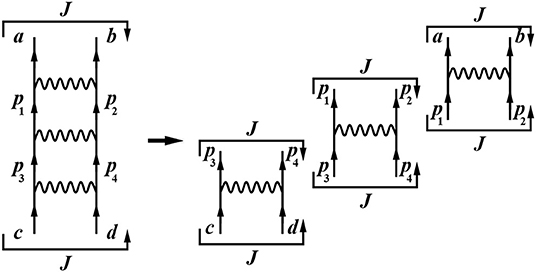
Figure 4. Two-body ladder diagram at third order in perturbation theory: lines with arrows represent incoming/outgoing and intermediate particle states; wavy lines represent interaction vertices.

The analytical expression for V_ladder is

\begin{array}{l} 〈 a, b; J | V_{ladder} | c, d; J 〉 \\ = + \frac{1}{4} \sum_{p_{1}, p_{2}, p_{3}, p_{4}} \frac{〈 a, b; J | V_{N N} | p_{1}, p_{2}; J 〉 〈 p_{1}, p_{2}; J | V_{N N} | p_{3}, p_{4}; J 〉 〈 p_{3}, p_{4}; J | V_{N N} | c, d; J 〉}{[ϵ_{0} - (ϵ_{p_{1}} + ϵ_{p_{2}})] [ϵ_{0} - (ϵ_{p_{3}} + ϵ_{p_{4}})]}, & (55) \end{array}

where ϵ_m denotes the unperturbed SP energy of the orbital j_m and ϵ₀ is the so-called starting energy, i.e., the unperturbed energy of the incoming particles, ϵ₀ = ϵ_c + ϵ_d.

We point out that the factor +1/4 is related to rules that characterize the calculation of overall factors in $\hat{Q}$ -box Goldstone diagrams; for any diagram we have a phase factor

{(- 1)}^{(n_{h} + n_{l} + n_{c} + n_{exh})}

whose value is determined by the total number of hole lines (n_h), the total number of closed loops (n_l), the total number of crossings of different external lines as they trace through the diagrams (n_c), and the total number of external hole lines that continuously trace through the diagrams (n_exh) [51]. There is also a factor of ${(1 / 2)}^{n_{ep}}$ , which accounts for the pairs of lines that start together from one interaction vertex and end together at another one (n_ep).

The diagram in Figure 4 has n_h = n_l = n_c = n_exh = 0, and consequently the phase is positive. The number of pairs of particles starting and ending together at the same vertices is n_ep = 2, and so the overall factor is +1/4.

The factorization of Goldstone diagrams, such as the ladder diagram in Figure 4 in terms of their interaction vertices is quite simple. There is a large class of diagrams, like the three-particle-one-hole diagram (3p-1h) in Figure 5, which require some additional considerations to obtain a straightforward factorization.

FIGURE 5

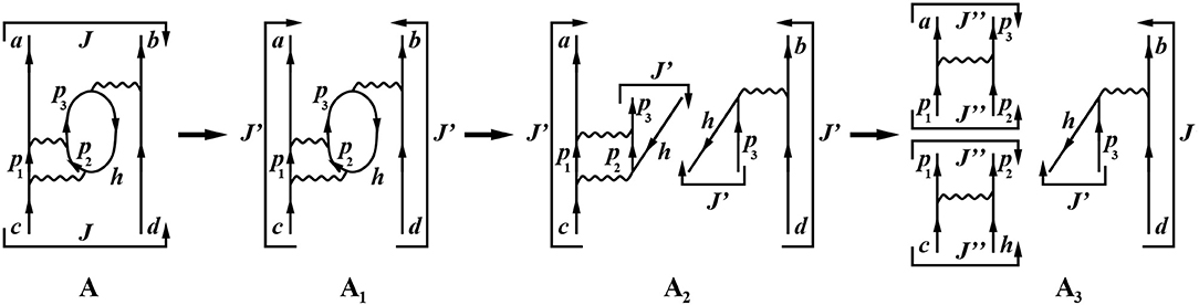
Figure 5. Two-body 3p-1h diagram at third order in perturbation theory: lines with arrows represent incoming/outgoing and intermediate particle/hole states; wavy lines indicate interaction vertices.

The factorization can easily be performed by taking into account the fact that the interaction operator V_NN transforms as a scalar under rotation, and so we introduce the following cross-coupling transformation of the TBMEs:

\begin{array}{l} {〈 a, b; J | V_{N N} | c, d; J 〉}_{CC} = \frac{1}{\hat{J}} \sum_{J^{'}} \hat{J^{'}} X (\begin{matrix} j_{c} & j_{a} & J \\ j_{d} & j_{b} & J \\ J^{'} & J^{'} & 0 \end{matrix}) \\ 〈 a, b; J^{'} | V_{N N} | c, d; J^{'} 〉, & (56) \end{array}

where $\hat{x} = {(2 x + 1)}^{1 / 2}$ and X is the so-called standard normalized 9-j symbol, expressed in terms of the Wigner 9-j symbol [54] as

X (\begin{matrix} r & s & t \\ u & v & w \\ x & y & z \end{matrix}) = \hat{t} \hat{w} \hat{x} \hat{y} {\begin{matrix} r & s & t \\ u & v & w \\ x & y & z \end{matrix}} .

The orthonormalization properties of X allow us to then write the direct-coupled TBMEs in terms of the cross-coupled TBMEs:

\begin{array}{l} 〈 a, b; J | V_{N N} | c, d; J 〉 = \frac{1}{\hat{J}} \sum_{J^{'}} \hat{J^{'}} X (\begin{matrix} j_{c} & j_{d} & J \\ j_{a} & j_{b} & J \\ J^{'} & J^{'} & 0 \end{matrix}) \\ {〈 a, b; J^{'} | V_{N N} | c, d; J^{'} 〉}_{CC} . & (57) \end{array}

Equations (56) and (57) help us to perform the factorization of the diagram in Figure 5. First, a rotation according to Equation (57) transforms the direct coupling to the total angular momentum J into the cross-coupled one J′ (diagram A going to diagram A₁ in Figure 5). This allows us to cut the inner loop and factorize the diagram into two terms, a ladder component (α) and a cross-coupled matrix element (β) (diagram A₂ in Figure 5):

\begin{array}{l} (α) = {〈 a, p_{3}; J^{'} | A | c, h; J^{'} 〉}_{CC}, \\ (β) = {〈 h, b; J^{'} | V_{N N} | p_{3}, d; J^{'} 〉}_{CC} . \end{array}

Next, we transform the ladder diagram (A) back to a direct coupling to J″ by way of Equation (56), and factorize it into the TBMEs (I) and (II) (diagram A₃ in Figure 5):

\begin{array}{l} (I) = 〈 a, p_{3}; J^{″} | V_{N N} | p_{1}, p_{2}; J^{″} 〉, \\ (II) = 〈 p_{1}, p_{2}; J^{″} | V_{N N} | c, h; J^{″} 〉 . \end{array}

The analytical expression for the diagram in Figure 5 is then

\begin{array}{l} 〈 a, b; J | V_{3 p 1 h} | c, d; J 〉 = - \frac{1}{2} \frac{1}{\hat{J}} \sum_{h, p_{1}, p_{2}, p_{3}} \sum_{J^{'}, J^{″}} \hat{J^{″}} X (\begin{matrix} j_{c} & j_{d} & J \\ j_{a} & j_{b} & J \\ J^{'} & J^{'} & 0 \end{matrix}) X (\begin{matrix} j_{c} & j_{a} & J^{'} \\ j_{h} & j_{p} & J^{'} \\ J^{″} & J^{″} & 0 \end{matrix}) \\ \times \frac{{〈 h, b; J^{'} | V_{N N} | p_{3}, d; J^{'} 〉}_{CC} 〈 a, p_{3}; J^{″} | V_{N N} | p_{1}, p_{2}; J^{″} 〉 〈 p_{1}, p_{2}; J^{″} | V_{N N} | c, h; J^{″} 〉}{[ϵ_{0} - (ϵ_{p_{1}} + ϵ_{p_{2}})] [ϵ_{0} - (ϵ_{p_{3}} + ϵ_{p_{4}})]}, & (58) \end{array}

The factor of −1/2 accounts for the facts that n_ep = 1, n_h = n_l = 1, and an extra phase factor ${(- 1)}^{n_{ph}}$ is needed for the total number of cuts of particle-hole pairs (n_ph) [51], since in order to factorize the diagram we have to cut the inner loop.

We remark that there are another three diagrams with the same topology as the one in Figure 5, which corresponds to the exchange of external incoming and outgoing particles.

Let us now turn our attention to one-body diagrams. First, we consider the contribution of diagrams, such as the one in Figure 6.

FIGURE 6

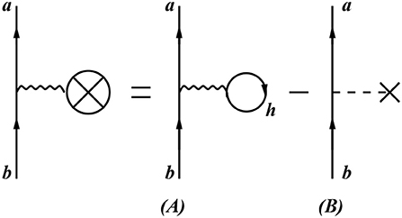
Figure 6. (V-U)-insertion diagram: graph A is the self-energy diagram, and graph B represents the matrix element of the harmonic oscillator potential $U = \frac{1}{2} m ω^{2} r^{2}$ .

The diagram in Figure 6 is the so-called (V-U)-insertion diagram and is composed of the self-energy diagram (V-insertion diagram) minus the auxiliary potential U-insertion. The U-insertion diagrams are due to the presence of the U term in H₁. The analytical expression for this diagram is

\begin{array}{l} 〈 a ‖ (V - U) ‖ b 〉 = \frac{δ_{j_{a} j_{b}}}{2 j_{a} + 1} \sum_{J, h} (2 J + 1) 〈 j_{a}, h; J | V | j_{b}, h; J 〉 - 〈 a ‖ U ‖ b 〉 \\ = \frac{δ_{j_{a} j_{b}}}{2 j_{a} + 1} \sum_{J, h} (2 J + 1) 〈 j_{a}, h; J | V | j_{b}, h; J 〉 - 〈 a ‖ \frac{1}{2} m ω^{2} r^{2} ‖ b 〉 . & (59) \end{array}

The calculation of the self-energy diagram A is performed by coupling the external lines to a scalar, which leads to the SP total angular momentum and the parity of j_a, j_b being identical. Then we cut the inner hole line and, since the SP states a and b are coupled to J = 0⁺, apply the transformation in Equation (56) with J = 0⁺.

Since the standard choice for the auxiliary potential is the harmonic oscillator potential, we also have the reduced matrix element of $U = \frac{1}{2} m ω^{2} r^{2}$ between the SP states a and b (graph B in Figure 6).

It is worth pointing out that the diagonal contributions of (V-U)-insertion diagrams, for SP states belonging to the model space, correspond to first-order contributions of the perturbative expansion of the effective SM Hamiltonian $H_{eff}^{1 b}$ of single-valence-nucleon systems.

Moreover, (V-U)-insertion diagrams turn out to be identically zero if a self-consistent Hartree-Fock (HF) auxiliary potential is used [40], and reference [52] discusses the important role played by these terms, comparing different effective Hamiltonians derived by starting from $\hat{Q}$ -boxes with and without contributions from (V-U)-insertion diagrams.

Now we will give an example of a one-body diagram and comment briefly on its analytical calculation. We consider the diagram in Figure 7; the complete list of third-order one-body diagrams can be found in reference [52], Figure B.19.

FIGURE 7

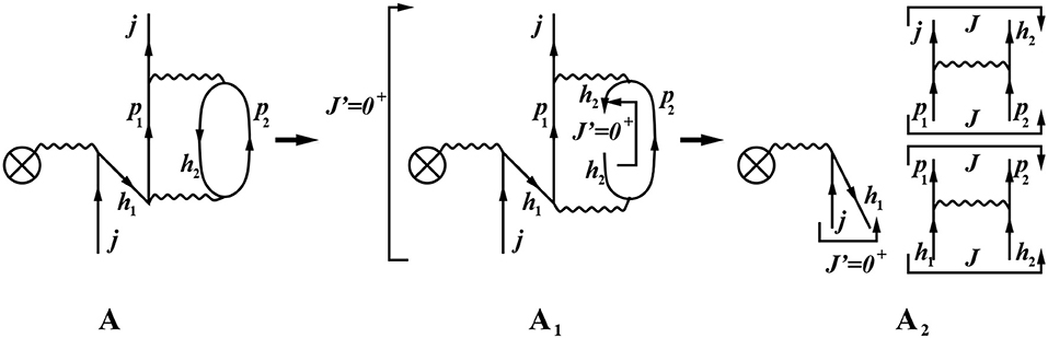
Figure 7. An example of a one-body diagram (see text for details).

We call this diagram V_2p1h, since between the upper interaction vertices two particles and one hole appear as intermediate states. This diagram belongs to the group of non-symmetric diagrams, which always occur in pairs that give equal contributions. Its analytical expression is

\begin{array}{l} 〈 j ‖ V_{2 p 1 h} ‖ j 〉 = - \frac{1}{2} \frac{1}{2 j + 1} \\ \sum_{\begin{matrix} J, p_{1}, p_{2}, \\ h_{1}, h_{2} \end{matrix}} (2 J + 1) \frac{〈 j, h_{2}; J | V_{N N} | p_{1}, p_{2}; J 〉 〈 p_{1}, p_{2}; J | V_{N N} | h_{1}, h_{2}; J 〉 〈 h_{1} ‖ V - U ‖ j 〉}{[ϵ_{0} - (ϵ_{p_{1}} + ϵ_{p_{2}} - ϵ_{h_{2}})] [ϵ_{0} - (ϵ_{j} + ϵ_{p_{1}} + ϵ_{p_{2}} - ϵ_{h_{1}} - ϵ_{h_{2}})]} & (60) \end{array}

where ϵ₀ = ϵ_j is the unperturbed SP energy of the incoming particle j.

To factorize the diagram, we first cross-couple the incoming and outgoing model-space states j to J′ = 0⁺ (diagram A₁ in Figure 7). Then we cut the hole line h₂ and, by way of Equation (56), obtain a sum of two-body diagrams which are direct-coupled to the total angular momentum J [51] (diagram A₂ in Figure 7). These operations are responsible for the factors 1/(2j + 1) and (2J + 1); the overall factor 1/2 is due to the pair of particle lines (p₁, p₂) starting and ending at the same vertices, while the minus sign comes from the two hole lines and one loop appearing in the diagram. The factorization also takes into account the (V-U)-insertion 〈h₁||V-U|j〉.

As mentioned before, this diagrammatic approach is valid for deriving H_eff for one- and two-valence-nucleon systems; the situation is different and more complicated if one wishes to derive H_eff for systems with three or more valence nucleons.

Actually, none of the available SM codes can perform diagonalization of SM Hamiltonians with three-body components; the exception is the BIGSTICK SM code [55], but it works only for light nuclei.

In order to incorporate the contribution to H_eff of $\hat{Q}$ -box diagrams with at least three incoming and outgoing valence particles, we resort to the so-called normal-ordering decomposition of the three-body component of a many-body Hamiltonian [56]. To this end, we also include in the calculation of the $\hat{Q}$ -box second-order three-body diagrams, which, for those nuclei with more than two valence nucleons, account for the interaction via the two-body force of the valence nucleons with core excitations as well as virtual intermediate nucleons scattered above the model space (see Figure 8).

FIGURE 8

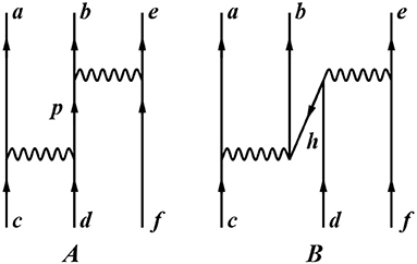
Figure 8. Second-order three-body diagrams. The sum over the intermediate lines runs over particle and hole states outside the model space, shown in A and B, respectively. For the sake of simplicity, for each topology we show only one of the diagrams which correspond to permutations of the external lines.

For each topology shown in Figure 8 there are nine diagrams, corresponding to the possible permutations of the external lines. The analytical expressions for the second-order three-body contributions are reported in reference [57], and we derive from those expressions a density-dependent two-body term.

To this end, for each (A, B) topology we calculate nine one-loop diagrams, i.e., graphs of the form α in Figure 9. Their explicit form, in terms of the three-body graphs (A, B), is

\begin{array}{l} 〈 {(j_{a} j_{b})}_{J} | V^{α} | {(j_{c} j_{d})}_{J} 〉 = \sum_{m, J^{'}} ρ_{m} \frac{{\hat{J^{'}}}^{2}}{{\hat{J}}^{2}} 〈 {[{(j_{a} j_{b})}_{J}, j_{m}]}_{J^{'}} | V^{A, B} | {[{(j_{c} j_{d})}_{J}, j_{m}]}_{J^{'}} 〉, & (61) \end{array}

where the summation over the index m runs over the model space and ρ_m is the unperturbed occupation density of the orbital m according to the number of valence nucleons.

FIGURE 9

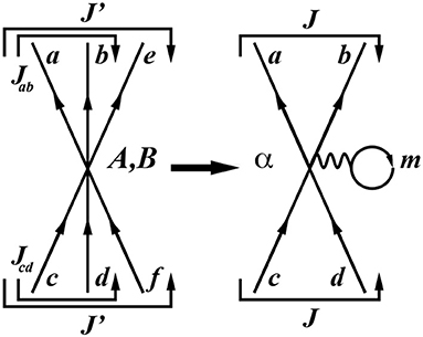
Figure 9. Density-dependent two-body contribution obtained from a three-body one; α is obtained by summing over one incoming and one outgoing particle of the three-body graphs A in Figure 8.

Finally, the perturbative expansion of the $\hat{Q}$ -box contains one- and two-body diagrams up to third order in V_NN, along with a density-dependent two-body contribution that accounts for three-body second-order diagrams [57, 58]. We point out that the latter term depends on the number of valence protons and neutrons, thus leading to the derivation of specific effective SM Hamiltonians that differ only in the two-body matrix elements.

3.3. Effective Shell-Model Decay Operators

In the SM approach, we are interested not only in calculating energies but also in finding the matrix elements of operators Θ that represent physical observables (such as electromagnetic transition rates, multipole moments, etc.).

Since the wave functions |ψ_α〉 obtained from diagonalizing H_eff are not the true ones |Ψ_α〉 but their projections onto the chosen model space (|ψ_α〉 = P|Ψ_α〉), it is obvious that one has to renormalize Θ to take into account the neglected degrees of freedom corresponding to the Q-space. In other words, one needs to consider the short-range correlation “wounds” inflicted by the bare interaction on the SM wave functions. Formally, one seeks to derive an effective operator Θ_eff such that

\begin{array}{l} 〈 {\tilde{Ψ}}_{α} | Θ | Ψ_{β} 〉 = 〈 {\tilde{ψ}}_{α} | Θ_{eff} | ψ_{β} 〉 . & (62) \end{array}

The perturbative expansion of effective operators has been studied since the earliest attempts to employ realistic potentials for SM calculations; among the many studies we mention the fundamental and pioneering work carried out by L. Zamick on the problem of electromagnetic transitions [59–61] and by I. S. Towner on the quenching of spin-operator matrix elements [62, 63].

In this subsection we discuss the formal structure of non-Hermitian effective operators, as introduced by Suzuki and Okamoto in reference [18]. More precisely, we give an expansion formula for the effective operators in terms of the $\hat{Θ}$ -box, which, analogous to the $\hat{Q}$ -box in the effective interaction theory (see section 3), is the building block for constructing effective operators.

According to Equation (20) (and keeping in mind that ω ≡ QωP), we may write H_eff as

\begin{array}{l} H_{eff} = P H (P + ω), & (63) \end{array}

so that we can express the true eigenstates |Ψ_α〉 and their orthonormal counterparts $〈 {\tilde{Ψ}}_{α} |$ as

\begin{array}{l} | Ψ_{α} 〉 = (P + ω) | ψ_{α} 〉, 〈 {\tilde{Ψ}}_{α} | = 〈 {\tilde{ψ}}_{α} | (P + ω^{†} ω) (P + ω^{†}) . & (64) \end{array}

On the other hand, a general effective operator expression in the bra-ket representation is

\begin{array}{l} Θ_{eff} = \sum_{α, β} | ψ_{α} 〉 〈 {\tilde{Ψ}}_{α} | Θ | Ψ_{β} 〉 〈 {\tilde{ψ}}_{β} |, & (65) \end{array}

where Θ is a general time-independent Hermitian operator. Therefore, we can write Θ_eff in operator form as

\begin{array}{l} Θ_{eff} = {(P + ω^{†} ω)}^{- 1} (P + ω^{†}) Θ (P + ω) . & (66) \end{array}

It is worth noting that Equation (62) holds independently of the normalization of |Ψ_α〉 and |ψ_α〉, but if the true eigenvectors are normalized, then $〈 {\tilde{Ψ}}_{α} | = 〈 Ψ_{α} |$ and the |ψ_α〉 should be normalized in the following way:

\begin{array}{l} 〈 {\tilde{ψ}}_{α} | (P + ω^{†} ω) | ψ_{α} 〉 = 1 . & (67) \end{array}

To explicitly calculate Θ_eff, we introduce the $\hat{Θ}$ -box, defined as

\begin{array}{l} \hat{Θ} = (P + ω^{†}) Θ (P + ω), & (68) \end{array}

so that Θ_eff can be factorized as

\begin{array}{l} Θ_{eff} = {(P + ω^{†} ω)}^{- 1} \hat{Θ} . & (69) \end{array}

The derivation of Θ_eff is divided into two steps: the calculation of $\hat{Θ}$ and the calculation of ω^†ω.

According to Equation (68) and taking into account the expression for ω in terms of H_eff, i.e.,

\begin{array}{l} ω = \sum_{n = 0}^{\infty} {(- 1)}^{n} {(\frac{1}{ϵ_{0} - Q H Q})}^{n + 1} Q H_{1} P {(H_{1}^{eff})}^{n}, & (70) \end{array}

we can write

\begin{array}{l} \hat{Θ} = {\hat{Θ}}_{P P} + ({\hat{Θ}}_{P Q} + h . c .) + {\hat{Θ}}_{Q Q}, & (71) \end{array}

where

\begin{array}{l} {\hat{Θ}}_{P P} = P Θ P, & (72) \end{array}

\begin{array}{l} {\hat{Θ}}_{P Q} = P Θ ω P = \sum_{n = 0}^{\infty} {\hat{Θ}}_{n} {(H_{1}^{eff})}^{n}, & (73) \end{array}

\begin{array}{l} {\hat{Θ}}_{Q Q} = P ω^{†} Θ ω P = \sum_{n, m = 0}^{\infty} {(H_{1}^{eff})}^{n} {\hat{Θ}}_{n m} {(H_{1}^{eff})}^{m}, & (74) \end{array}

and ${\hat{Θ}}_{m}$ and ${\hat{Θ}}_{m n}$ are given by

\begin{array}{l} {{\hat{Θ}}_{m} = \frac{1}{m!} \frac{d^{m} \hat{Θ} (ϵ)}{d ϵ^{m}} |}_{ϵ = ϵ_{0}}, & (75) \end{array}

\begin{array}{l} {{\hat{Θ}}_{m n} = \frac{1}{m! n!} \frac{d^{m}}{d ϵ_{1}^{m}} \frac{d^{n}}{d ϵ_{2}^{n}} \hat{Θ} (ϵ_{1}; ϵ_{2}) |}_{ϵ_{1} = ϵ_{0}, ϵ_{2} = ϵ_{0}} & (76) \end{array}

with

\begin{array}{l} \hat{Θ} (ϵ) = P Θ P + P Θ Q \frac{1}{ϵ - Q H Q} Q H_{1} P, & (77) \end{array}

\begin{array}{l} \hat{Θ} (ϵ_{1}; ϵ_{2}) = P H_{1} Q \frac{1}{ϵ_{1} - Q H Q} Q Θ Q \frac{1}{ϵ_{2} - Q H Q} Q H_{1} P . & (78) \end{array}

As regards the product ω^†ω, using the definition (31) we can write

\begin{array}{l} ω^{†} ω = - \sum_{n = 1}^{\infty} \sum_{m = 1}^{\infty} {({(H_{1}^{eff})}^{†})}^{n - 1} \hat{Q} {(ϵ_{0})}_{n + m - 1} {(H_{1}^{eff})}^{m - 1} . & (79) \end{array}

Upon expressing $H_{1}^{eff}$ in terms of the $\hat{Q}$ -box and its derivatives (see Equations 33 and 34), the above quantity may be rewritten as

\begin{array}{l} ω^{†} ω = - {\hat{Q}}_{1} + ({\hat{Q}}_{2} \hat{Q} + h . c .) + ({\hat{Q}}_{3} \hat{Q} \hat{Q} + h . c .) \\ + ({\hat{Q}}_{2} {\hat{Q}}_{1} \hat{Q} + h . c .) + \dots . & (80) \end{array}

Putting together Equations (77) and (80), we can write the final perturbative expansion of the effective operator Θ_eff:

\begin{array}{l} Θ_{eff} = (P + {\hat{Q}}_{1} + {\hat{Q}}_{1} {\hat{Q}}_{1} + {\hat{Q}}_{2} \hat{Q} + \hat{Q} {\hat{Q}}_{2} + \dots) \times (χ_{0} + χ_{1} + χ_{2} + \dots), & (81) \end{array}

where

\begin{array}{l} χ_{0} = ({\hat{Θ}}_{0} + h . c .) + {\hat{Θ}}_{00}, & (82) \end{array}

\begin{array}{l} χ_{1} = ({\hat{Θ}}_{1} \hat{Q} + h . c .) + ({\hat{Θ}}_{01} \hat{Q} + h . c .), & (83) \end{array}

\begin{array}{l} χ_{2} = ({\hat{Θ}}_{1} {\hat{Q}}_{1} \hat{Q} + h . c .) + ({\hat{Θ}}_{2} \hat{Q} \hat{Q} + h . c .) \\ + ({\hat{Θ}}_{02} \hat{Q} \hat{Q} + h . c .) + \hat{Q} {\hat{Θ}}_{11} \hat{Q} . \\ ⋮ & (84) \end{array}

It is worth elucidating the strong link that exists between H_eff and any effective operator. This is achieved by inserting the identity $\hat{Q} {\hat{Q}}^{- 1} = 1$ into Equation (81) to obtain the following expression:

\begin{array}{l} Θ_{eff} = (P + {\hat{Q}}_{1} + {\hat{Q}}_{1} {\hat{Q}}_{1} + {\hat{Q}}_{2} \hat{Q} + \hat{Q} {\hat{Q}}_{2} + \dots) \hat{Q} {\hat{Q}}^{- 1} \\ \times (χ_{0} + χ_{1} + χ_{2} + \dots) \\ = H_{eff} {\hat{Q}}^{- 1} (χ_{0} + χ_{1} + χ_{2} + \dots) . & (85) \end{array}

In actual calculations the χ_n series is truncated to a finite order and the starting point is the derivation of perturbative expansions for ${\hat{Θ}}_{0} \equiv \hat{Θ} (ϵ_{0})$ and ${\hat{Θ}}_{00} \equiv \hat{Θ} (ϵ_{0}; ϵ_{0})$ , including diagrams up to a finite order in the perturbation theory, consistently with the expansion of the $\hat{Q}$ -box. The issue of convergence of the χ_n series and of the perturbative expansions of ${\hat{Θ}}_{0}$ and ${\hat{Θ}}_{00}$ will be treated extensively in section 4.1.

In Figure 10 we display all the diagrams up to second order appearing in the ${\hat{Θ}}_{0}$ expansion for a one-body operator Θ.

FIGURE 10

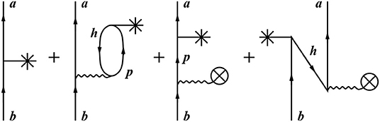
Figure 10. One-body second-order diagrams included in the perturbative expansion of ${\hat{Θ}}_{0}$ ; an asterisk indicates the bare operator Θ.

The evaluation of the diagrams involved in the derivation of Θ_eff follows the same procedure as described in the previous section. Therefore, in the following we will just outline the procedure for calculating such diagrams with one Θ vertex.

Let us suppose that the operator Θ transforms like a spherical tensor of rank λ and with component μ:

\begin{array}{l} Θ \equiv T_{μ}^{λ}, & (86) \end{array}

with

\begin{array}{l} {(T_{μ}^{λ})}^{†} = {(- 1)}^{λ - μ} T_{- μ}^{λ} . & (87) \end{array}

By using the Wigner-Eckart theorem, it is possible to express any transition matrix element in terms of a reduced transition element:

\begin{array}{l} 〈 j_{a} ‖ T^{λ} ‖ j_{b} 〉 = {(- 1)}^{λ - μ} 〈 j_{a} | T_{μ}^{λ} | j_{b} 〉, & (88) \end{array}

where in the right-hand side j_b and j_a are coupled to a total angular momentum and projection equal to λ and −μ, respectively, and we have assumed without lack of generality that we are dealing with single-particle states.

Therefore, we evaluate each diagram as a contribution to the reduced matrix element of the effective operator. To be more explicit, we consider as an example the calculation of the following second-order diagram that takes into account the renormalization of the operator due to 1p-1h core excitations.

The first step is to couple j_b and j_a to a total angular momentum equal to λ. This enables us to factorize the diagram as the product of a cross-coupled matrix element of the interaction and the reduced matrix element of the operator (see the right-hand part of Figure 11).

FIGURE 11

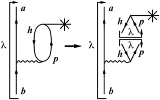
Figure 11. One-body second-order 2p-1h diagram included in the perturbative expansion of ${\hat{Θ}}_{0}$ ; an asterisk indicates the bare operator Θ.

Explicitly, we can evaluate the diagram as

\begin{array}{l} 〈 j_{a} ‖ Θ_{2 p 1 h} ‖ j_{b} 〉 \\ = - \sum_{p, h} {(- 1)}^{j_{p} + j_{h} - λ} \frac{{〈 j_{a}, p; λ | V_{N N} | j_{b}, h; λ 〉}_{CC} 〈 h ‖ T^{λ} ‖ p 〉}{ϵ_{0} - (ϵ_{a} + ϵ_{b} - ϵ_{h})} . & (89) \end{array}

The minus sign in front is due to the fact that n_h = n_l = 1 and that an extra phase factor ${(- 1)}^{n_{ph}}$ is needed for the total number of cuts of particle-hole pairs (n_ph) [51], since we have to cut the inner loop to factorize the diagram.

4. Applications

In this section we present a specific example of SM calculations performed by employing effective SM Hamiltonian and decay operators derived from realistic nuclear potentials within the many-body perturbation theory.

These kinds of calculations have actually been carried out since the mid-1960s, but they mostly involved retaining only the TBMEs, since the single-body components of H_eff were not considered accurate enough to provide SM results that would agree well with experiments. A large sample of calculations performed in that successful framework can be found in previous reviews of the topic [6, 7].

Here we present results of a calculation where both the SP energies and the TBMEs that are needed to diagonalize the SM Hamiltonian have been obtained by deriving H_eff according to the procedures described in the previous section. Besides H_eff, the many-body perturbation theory has been used to derive consistently effective operators to calculate electromagnetic transition rates and Gamow-Teller (GT) strengths without resorting to the use of empirical effective charges or quenching factors for the axial coupling constant g_A.

The following are some motivations for performing SM calculations by deriving and employing all SM parameters—SP energies, TBMEs, and effective transition and decay operators—starting from realistic nuclear forces:

• the need to study the soundness of many-body perturbation theory so as to provide reliable SM parameters;

• the need to determine the ability of classes of nuclear potentials to describe nuclear structure observables;

• the opportunity to compare and benchmark SM calculations against other nuclear structure methods that employ realistic potentials.

The goal of these studies is to assess the reliability of such an approach to investigating the nuclear SM, especially its predictiveness, which is crucial for describing physical phenomena that are not yet accessible experimentally.

4.1. The Double-β Decay Around Doubly Closed ¹³²Sn

Neutrinoless double-β (0νββ) decay is an exotic second-order electroweak process predicted by extensions of the Standard Model of particle physics. Observation of such a process would demonstrate the non-conservation of the lepton number and provide evidence that neutrinos have a Majorana mass component (see references [64, 65] and references therein).

In the framework of light-neutrino exchange, the half-life of the 0νββ decay is inversely proportional to the square of the effective Majorana neutrino mass 〈m_ν〉:

\begin{array}{l} {[T_{1 / 2}^{0 ν}]}^{- 1} = G^{0 ν} {| M^{0 ν} |}^{2} g_{A}^{4} | \frac{〈 m_{ν} 〉}{m_{e}} |^{2}, & (90) \end{array}

where g_A is the axial coupling constant, m_e is the electron mass, G^0ν is the so-called phase-space factor (or kinematic factor), and M^0ν is the nuclear matrix element (NME), which is related to the wave functions of the nuclei involved in the decay.

At present, the phase-space factors for nuclei that are possible candidates for 0νββ decay can be calculated with great accuracy [66, 67]. It is therefore crucial to have precise values for the NME, both to improve the reliability of the 0νββ lifetime predictions—a fundamental ingredient in the design of new experiments—and to extract neutrino properties from the experimental results, when they become available.

Several nuclear structure models have been exploited to provide NME values that are as precise as possible, the most commonly used being the interacting boson model [68–70], the quasiparticle random-phase approximation [71–74], energy density functional methods [75], the covariant density functional theory [76–78], the generator-coordinate method [79–82], and the shell model [83–87].

All of the above models use a truncated Hilbert space to reduce the computational complexity, and each can be more efficient than the others for a specific class of nuclei. However, when comparing the calculated NMEs obtained via different approaches, it is seen that, at present, the results can differ by a factor of two or three (see for instance the review in reference [88]).

Reference [89] reports on the calculation of the 0νββ-decay NME for ⁴⁸Ca, ⁷⁶Ge, ⁸²Se, ¹³⁰Te, and ¹³⁶Xe in the framework of the realistic SM, where the H_eff's and 0νββ-decay effective operators are consistently derived starting from a realistic NN potential, the high-precision CD-Bonn potential [90].

We remark that the above work is not the first example of such an approach, which was pioneered by Kuo and coworkers [91, 92] and more recently pursued by Holt and Engel [93].

Here we restrict ourselves to the results obtained in reference [89] for the heavy-mass nuclei around ¹³²Sn, ¹³⁰Te, and ¹³⁶Xe. At present, these nuclei are under investigation as 0νββ-decay candidates by some large experimental collaborations. The possible 0νββ decay of ¹³⁰Te is being studied by the CUORE collaboration at the INFN Laboratori Nazionali del Gran Sasso in Italy [94], while ¹³⁶Xe is being investigated by both the EXO-200 collaboration at the Waste Isolation Pilot Plant in Carlsbad, New Mexico [95], and the KamLAND-Zen collaboration at the Kamioka mine in Japan [96].

The starting point of the SM calculation is the high-precision CD-Bonn NN potential [90], whose non-perturbative behavior induced by its repulsive high-momentum components is treated with the so-called V_low-k approach [97]. This yields a smooth potential which exactly preserves the onshell properties of the original NN potential up to a chosen cutoff momentum Λ. As in other SM studies [98–101], the value of the cutoff has been chosen as Λ = 2.6 fm⁻¹, since the role of the missing three-nucleon force (3NF) decreases as the V_low-k cutoff is increased [99]. In fact, in reference [99] it is shown that H_eff's derived from V_low-k's with small cutoffs (Λ = 2.1 fm⁻¹) have SP energies that are in worse agreement with experiments, as well as unrealistic shell-evolution behavior. This may be attributed to a greater impact of the induced 3NF, which becomes less important with a larger cutoff.

In our experience, Λ = 2.6 fm⁻¹, within a perturbative expansion of the $\hat{Q}$ -box, is an upper limit, since a larger cutoff worsens the order-by-order behavior of the perturbative expansion; at the end of this section we report a study of the perturbative properties of H_eff and of the effective decay operators derived using this V_low-k potential.

The Coulomb potential is explicitly taken into account in the proton-proton channel.

The SM effective Hamiltonian H_eff is derived within the framework of the many-body perturbation theory as described in section 3, including diagrams up to third order in H₁ in the $\hat{Q}$ -box -expansion, while all the effective operators, both one- and two-body, are obtained consistently using the approach described in section 3.3, including diagrams up to third order in perturbation theory in the evaluation of the $\hat{Θ}$ -box and truncating the χ_n series in Equation (81) to χ₂.

The effective Hamiltonian and operators are defined in a model space spanned by the five proton and neutron orbitals, 0g_7/2, 1d_5/2, 1d_3/2, 2s_1/2, and 0h_11/2, outside the doubly closed ¹⁰⁰Sn core. The SP energies and TBMEs of H_eff can be found in reference [101].

Before showing the results for the 0νββ NME obtained in reference [89], it is worth checking the reliability of the approach we have adopted. To this end, we present some results obtained from the calculation of quantities for which there exist experimental counterparts to compare with. In particular, we show selected results for the electromagnetic properties, GT strength distributions, and 2νββ decays in ¹³⁰Te and ¹³⁶Xe, which have been reported in references [101, 102].

Figures 12, 13 show experimental [103, 104] and calculated low-energy spectra and B(E2) strengths of parent and granddaughter nuclei involved in double-β decay of ¹³⁰Te and ¹³⁶Xe, respectively.

FIGURE 12

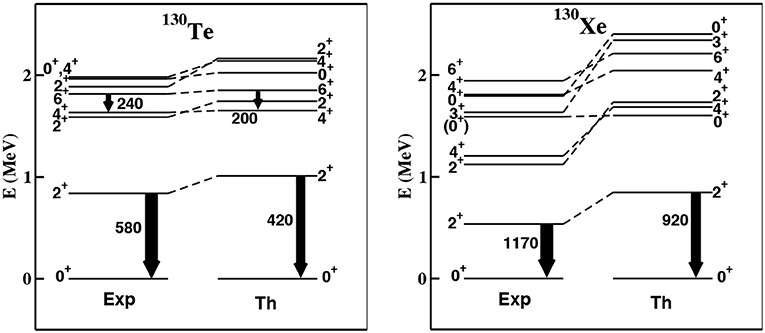
Figure 12. Experimental and calculated spectra of ¹³⁰Te and ¹³⁰Xe; the arrows are proportional to the B(E2) strengths, whose values are reported in e²fm⁴. Reproduced from reference [102].

FIGURE 13

Figure 13. Same as Figure 12 but for ¹³⁶Xe and ¹³⁶Ba. Reproduced from reference [102].

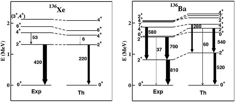
By inspection of Figures 12, 13 it can be seen that, as regards the low-lying excited states and the B(E2) transition rates, theory and experiment agree quite well for ¹³⁰Te, ¹³⁶Xe, and ¹³⁶Ba, but less so for ¹³⁰Xe, whose theoretical spectrum is expanded compared with the observed one. As regards the electromagnetic properties, in reference [102] they are calculated along with some B(M1) strengths and magnetic dipole moments using an effective spin-dependent M1 operator, and comparison with the available data (see Tables VII and IX in reference [102]) shows good agreement.

Two kinds of experimental data related to GT decay are available for ¹³⁰Te and ¹³⁶Xe: GT strength distributions and the NMEs involved in 2νββ decays. The GT strength B(GT) can be extracted from the GT component of the cross-section at zero degrees of intermediate energy charge-exchange reactions, following the standard approach in the distorted-wave Born approximation [105, 106]:

\begin{array}{l} \frac{d σ^{GT} (0 °)}{d Ω} = {(\frac{μ}{π ℏ^{2}})}^{2} \frac{k_{f}}{k_{i}} N_{D}^{σ τ} | J_{σ τ} |^{2} B (GT), & (91) \end{array}

where $N_{D}^{σ τ}$ is the distortion factor, |J_στ| is the volume integral of the effective NN interaction, k_i and k_f are the initial and final momenta, respectively, and μ is the reduced mass.

On the other hand, the experimental 2νββ NME $M_{GT}^{2 ν}$ can be extracted from the observed half-life $T_{1 / 2}^{2 ν}$ of the parent nucleus as follows:

\begin{array}{l} {[T_{1 / 2}^{2 ν}]}^{- 1} = G^{2 ν} | M_{GT}^{2 ν} |^{2} . & (92) \end{array}

Both of the above quantities can be calculated in terms of the matrix elements of the GT⁻ operator $\vec{σ} τ^{-}$ :

\begin{array}{l} B (GT) = \frac{| 〈 Φ_{f} ‖ \sum_{j} {\vec{σ}}_{j} τ_{j}^{-} ‖ Φ_{i} 〉 |^{2}}{2 J_{i} + 1}, & (93) \end{array}

\begin{array}{l} M_{GT}^{2 ν} = \sum_{n} \frac{〈 0_{f}^{+} ‖ \vec{σ} τ^{-} ‖ 1_{n}^{+} 〉 〈 1_{n}^{+} ‖ \vec{σ} τ^{-} ‖ 0_{i}^{+} 〉}{E_{n} + E_{0}}, & (94) \end{array}

where E_n is the excitation energy of the $J^{π} = 1_{n}^{+}$ intermediate state and $E_{0} = \frac{1}{2} Q_{β β} (0^{+}) + Δ M$ , with $Q_{β β} (0^{+})$ and ΔM being the Q-value of the ββ decay and the mass difference between the daughter and parent nuclei, respectively. The nuclear matrix elements in Equations (93) and (94) are calculated within the long-wavelength approximation, including only the leading order of the GT operator in a non-relativistic reduction of the hadronic current.

In reference [102] the GT strength distributions and 2νββ NMEs were calculated for ¹³⁰Te and ¹³⁶Xe using an effective spin-isospin-dependent GT operator, derived in a manner consistent with H_eff by following the procedure described in section 3.3.

Figure 14 shows the theoretical running sums of the GT strengths ΣB(GT), calculated with both bare and effective GT operators, plotted against the excitation energy and compared with the available data extracted from (³He, t) charge-exchange experiments [107, 108] for ¹³⁰Te and ¹³⁶Xe. It can be seen that in both nuclei, the GT strength distributions calculated using the bare GT operator overestimate the experimental ones by more than a factor of two. Including the many-body renormalization of the GT operator brings the predicted GT strength distribution into much better agreement with that extracted from experimental data.

FIGURE 14

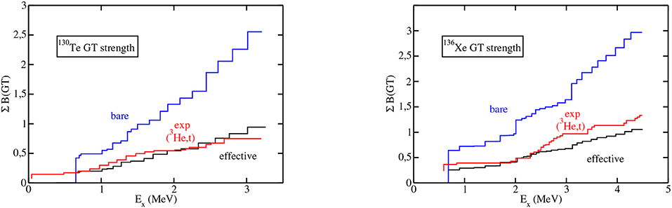
Figure 14. Running sums of the B(GT) strengths as a function of the excitation energy E_x up to 3 and 4.5 MeV, respectively, for ¹³⁰Te and ¹³⁶Xe. Reproduced from reference [102].

In reference [102] the NMEs $M_{GT}^{2 ν}$ involved in the decay of ¹³⁰Te and ¹³⁶Xe are calculated using the definition in Equation (94), by means of the Lanczos strength function method as in reference [3]. The results obtained with the bare GT operator and with the effective one are reported in Table 1 and compared with experimental values [109].

TABLE 1

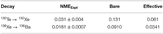
Table 1. Experimental [109] and calculated NMEs (in MeV⁻¹) of the 2νββ decay for ¹³⁰Te and ¹³⁶Xe.

The effective operator induces a relevant quenching of the calculated NME, 47% for ¹³⁰Te and 37% for ¹³⁶Xe decay, leading to fairly good agreement with the experimental value for both nuclei, of the same quality as for other SM calculations where all parameters (SP energies and TBMEs) were fitted to experimental values and a quenching factor q was introduced to reproduce GT data (see, for example, reference [110]). The overall agreement between theory and experiment shows that the many-body perturbation theory can be used to derive consistently effective Hamiltonians and transition operators that are able to reproduce quantitatively the observed spectroscopic and decay properties, without having to resort to any empirical adjustments, such as quenching of the axial coupling constant g_A. This supports the reliability of this approach to calculating the NMEs involved in 0νββ, the results of which were reported in reference [89] and are briefly summarized in the following.

The 0νββ two-body operator for the light-neutrino scenario can be expressed in the closure approximation (see e.g., references [111, 112]) in terms of the neutrino potentials H_α and form functions h_α(q) (α= F, GT, or T) as

\begin{array}{l} Θ_{GT} = {\vec{σ}}_{1} \cdot {\vec{σ}}_{2} H_{GT} (r) τ_{1}^{-} τ_{2}^{-}, & (95) \end{array}

\begin{array}{l} Θ_{F} = H_{F} (r) τ_{1}^{-} τ_{2}^{-}, & (96) \end{array}

\begin{array}{l} Θ_{T} = [3 ({\vec{σ}}_{1} \cdot \hat{r}) ({\vec{σ}}_{1} \cdot \hat{r}) - {\vec{σ}}_{1} \cdot {\vec{σ}}_{2}] H_{T} (r) τ_{1}^{-} τ_{2}^{-}, & (97) \end{array}

where

\begin{array}{l} H_{α} (r) = \frac{2 R}{π} \int_{0}^{\infty} \frac{j_{n_{α}} (q r) h_{α} (q^{2}) q d q}{q + 〈 E 〉} . & (98) \end{array}

The value of the parameter R is 1.2 A^1/3 fm, and the j_{n_α}(qr) are the spherical Bessel functions, with n_α = 0 for the Fermi and GT components and n_α = 2 for the tensor one. The explicit expressions for the neutrino form functions h_α(q) can be found in reference [89], and the average energies 〈E〉 are evaluated as in references [111, 112].

Apart from effects related to sub-nucleonic degrees of freedom, which were not accounted for in reference [89], the 0νββ-decay operator has to be renormalized to take into account both the degrees of freedom that are neglected in the adopted model space and the contribution of short-range correlations (SRCs). The latter arise because the action of a two-body decay operator on an unperturbed (uncorrelated) wave function, such as the one used in the perturbative expansion of Θ_eff, differs from the action of the same operator on the real (correlated) nuclear wave function.

It is worth pointing out that the calculations for 2νββ decay are not affected by this renormalization, since, as mentioned before, we retain only the leading order of the long-wavelength approximation, which corresponds to a zero-momentum-exchange (q = 0) process. On the other hand, the inclusion of higher-order contributions or corrections due to the sub-nucleonic structure of the nucleons [113–116] would connect high- and low-momentum configurations, and this renormalization should be carried out for the two-neutrino emission decay too.

In reference [117] the inclusion of SRCs was realized by means of an original approach [117] that is consistent with the V_low-k procedure. The 0νββ operator Θ, expressed in the momentum space, is renormalized by the same similarity transformation operator Ω_low-k that defines the V_low-k potential. This enables us to effectively take into account the high-momentum (short-range) components of the NN potential, in a framework where their direct contribution is not explicitly considered above a cutoff Λ. The resulting Θ_low-k vertices are then employed in the perturbative expansion of the $\hat{Θ}$ -box to calculate Θ_eff using Equation (85). More precisely, the perturbative expansion considers diagrams up to third order in perturbation theory, including those related to the so-called Pauli blocking effect (see Figure 2 in reference [89]), and the χ_n series is truncated to χ₂.

In reference [89] the contribution of the tensor component of the neutrino potential (Equation 97) is neglected, and therefore the total NME M^0ν is expressed as

\begin{array}{l} M^{0 ν} = M_{GT}^{0 ν} - {(\frac{g_{V}}{g_{A}})}^{2} M_{F}^{0 ν}, & (99) \end{array}

where g_A = 1.2723, g_V = 1 [118], and the matrix elements between the initial and final states $M_{α}^{0 ν}$ are calculated within the closure approximation

\begin{array}{l} M_{α}^{0 ν} = \sum_{j_{n}, j_{n^{'}}, j_{p}, j_{p^{'}}} 〈 f | a_{p}^{†} a_{n} a_{p^{'}}^{†} a_{n^{'}} | i 〉 \times 〈 j_{p} j_{p^{'}} ∣ Θ_{α} ∣ j_{n} j_{n^{'}} 〉 . & (100) \end{array}

The NMEs calculated using the 0νββ-decay effective operator are reported in Table 2 and compared with the values obtained using the bare operator without any renormalization.

TABLE 2

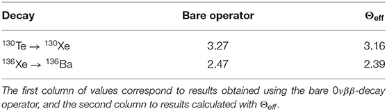
Table 2. Calculated values of M^0ν for ¹³⁰Te and ¹³⁶Xe decay.

The most striking feature that can be inferred from inspection of Table 2 is that the effects of the renormalization of the 0νββ-decay operator are far less relevant than those observed in the 2νββ-decay case.

A long-standing issue related to the calculation of M^0ν is possible interplay between the derivation of the effective one-body GT operator and the renormalization of the two-body GT component of the 0νββ operator, with some authors assuming that the same empirical quenching used to reproduce the observed GT-decay properties (single-β decay strengths, $M_{GT}^{2 υ}$ 's, etc.) should also be employed to calculate M^0ν (see for instance references [119, 120]). In fact, comparison of the results in Tables 1, 2 shows that the mechanisms underlying the microscopic derivation of the one-body single-β and the two-body 0νββ-decay effective operators lead to a considerably different renormalization, at variance with the above hypothesis.

The SM calculations of this section have been performed by employing, as interaction vertices of the perturbative expansion of the $\hat{Q}$ -box, a realistic potential derived from the high-precision CD-Bonn NN potential [90]. This potential is characterized by strong repulsive behavior in the high-momentum regime, so, as mentioned before, it is renormalized by deriving a low-momentum NN potential using the V_low-k approach [97].

As in other SM studies [98–101], the value of the cutoff is chosen as Λ = 2.6 fm⁻¹, since the role of the missing 3NF decreases as the V_low-k cutoff is increased [99]. This value, within a perturbative expansion of the $\hat{Q}$ -box, is an upper limit, since a larger cutoff worsens the order-by-order behavior of the perturbative expansion. Here, we discuss some implications for the properties of the perturbative expansion of H_eff and the SM effective transition operator when this “hard” V_low-k is employed to derive the SM Hamiltonian and operators.

Studies of the perturbative properties of the SP energy spacings and TBMEs are reported in references [99, 121], where H_eff is derived within the model space outside ¹³²Sn starting from the “hard” V_low-k. reference [122] contains a systematic investigation of the convergence properties of theoretical SP energy spectra, TBMEs, and 2νββ NMEs as functions of both the dimension of the intermediate state space and the order of the perturbative expansion. Moreover, reference [89] discusses convergence properties of the perturbative expansion of the effective 0νββ-decay operator with respect to the number of intermediate states and the truncation of both the order of the χ_n operators and the perturbative order of the diagrams. Here, we briefly sketch these results in order to assess the reliability of realistic SM calculations performed starting from a “hard” V_low-k.

The model space employed for the SM calculations in reference [122] is spanned by the five proton and neutron orbitals outside the doubly closed ¹⁰⁰Sn, namely 0g_7/2, 1d_5/2, 1d_3/2, 2s_1/2, and 0h_11/2, to study the 2νββ decay of ¹³⁰Te and ¹³⁶Xe.

The left panel of Figure 15 shows the behavior of the calculated SP spectrum of ¹⁰¹Sn with respect to the 0g_7/2 SP energy as a function of the maximum allowed excitation energy of the intermediate states expressed in terms of the oscillator quanta N_max. It is clear that convergence is achieved at N_max = 14, which, for the perturbative expansion of the effective SM Hamiltonian and decay operators, justifies the decision to include intermediate states with an unperturbed excitation energy of up to E_max = N_maxℏω where N_max = 16 [89, 101, 102, 122].

FIGURE 15

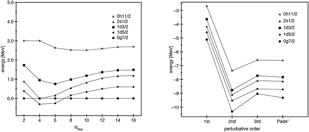
Figure 15. Neutron SP energies as a function of N_max (left) and of the perturbative order (right). Reproduced from reference [122] under the Creative Commons CC BY license.

As regards the order-by-order convergence of the SP energies, the right panel of Figure 15 plots the calculated neutron SP energies, using a number of intermediate states corresponding to N_max = 16, against the order of the perturbative expansion up to third order. The calculated neutron SP energies are also compared with the Padé approximant [2|1] of the $\hat{Q}$ -box, which estimates the value to which the perturbative series may converge. The results at third order are very close to those obtained with the Padé approximant, indicating that the truncation to third order should provide a reasonable estimate for the sum of the series.

As regards the TBMEs, we plot in Figure 16 the neutron-neutron diagonal J^π = 0⁺ TBMEs as a function both of N_max and of the perturbative order. These TBMEs, which contain the pairing properties of the effective Hamiltonian, are the largest in size of the calculated matrix elements and the most sensitive to the behavior of the perturbative expansion.

FIGURE 16

Figure 16. Neutron-neutron diagonal J^π = 0⁺ TBMEs as a function of N_max (left) and of the perturbative order (right). Reproduced from reference [122] under the Creative Commons CC BY license.

From Figure 16, the convergence with respect to N_max seems to be very fast for the diagonal matrix elements ${(1 d_{5 / 2})}^{2}$ , ${(1 d_{3 / 2})}^{2}$ , and ${(2 s_{1 / 2})}^{2}$ , whereas elements corresponding to orbitals that lack their own spin-orbit partner, i.e., ${(0 g_{7 / 2})}^{2}$ and ${(0 h_{11 / 2})}^{2}$ , show slower convergence. The order-by-order convergence seen in Figure 16 is quite satisfactory, and again the results at third order are very close to those obtained with the Padé approximant. Therefore, we can conclude that H_eff calculated from a V_low-k with cutoff equal to 2.6 fm⁻¹ by way of a perturbative expansion truncated at third order is a good estimate of the sum of its perturbative expansion, for both the one-body and the two-body components.

We now turn our attention to the perturbative expansion of the GT effective operator GT_eff. The selection rules of the GT operator that characterize a spin-isospin-dependent decay drive fast convergence of the matrix elements of its SM effective operator with respect to N_max. In fact, if the perturbative expansion is truncated at second order, their values do not change from N_max = 2 onward [62]; and at third order in perturbation theory, their third decimal digit values do not change from N_max = 12 onward.

Table 3 reports the calculated NMEs of the 2νββ decays ${}^{130}{Te}_{g . s .} \to {}^{130}{Xe}_{g . s .} and {}^{136}{Xe}_{g . s .} \to {{}^{136}B a}_{g . s .}$ obtained with effective operators at first, second, and third order in perturbation theory [with the χ_n series in Equation (85) truncated to χ₀] and compares them with experimental results [109].

TABLE 3

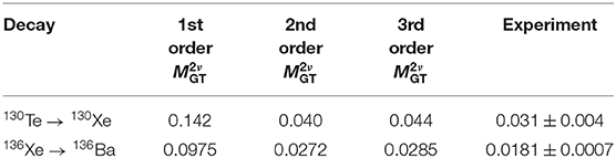
Table 3. Order-by-order $M_{GT}^{2 υ}$ 's (in MeV⁻¹) for ¹³⁰Te and ¹³⁶Xe [122].

As can be seen, the order-by-order convergence of the $M_{GT}^{2 υ}$ 's is also very satisfactory; for both transitions the results change by about 260% from the first- to the second-order calculations, while the changes are 9 and 5% from the second- to third-order results for the ¹³⁰Te and ¹³⁶Xe decays, respectively. This suppression of the third-order contributions relative to the second-order ones is favored by the mutual cancelation of third-order diagrams.

In reference [89] a study was also conducted on the convergence properties of the effective decay operator Θ_eff for the 0νββ decay with respect to the truncation of the χ_n operators, the number of intermediate states accounted for in the perturbative expansion, and the order-by-order behavior up to third order in perturbation theory.

Figure 17 displays the calculated values of M^0ν for the ⁷⁶Ge → ⁷⁶Se decay as a function of the maximum allowed excitation energy of the intermediate states expressed in terms of the oscillator quanta N_max, including χ_n contributions up to n = 2. We can see that the M^0ν values are convergent from N_max = 12 onward and that contributions from χ₁ are quite relevant, whereas those from χ₂ can be considered negligible.

FIGURE 17

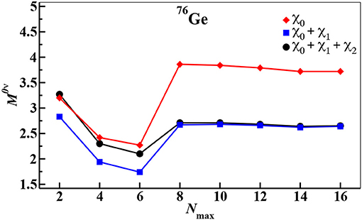
Figure 17. Calculated M^0ν values for the ⁷⁶Ge → ⁷⁶Se decay as a function of N_max: shown are truncations of the χ_n expansion up to χ₀ (red diamonds), up to χ₁ (blue squares), and up to χ₂ (black dots). Reproduced from reference [89].

We point out that, according to expression (84), χ₃ is defined in terms of the first, second, and third derivatives of ${\hat{Θ}}_{0}$ and ${\hat{Θ}}_{00}$ , as well as the first and second derivatives of the $\hat{Q}$ -box. This means that one could estimate χ₃ as being about one order of magnitude smaller than the χ₂ contribution.

On the above grounds, in reference [89] the effective SM 0νββ-decay operator was obtained by including in the perturbative expansion diagrams of up to third order, with the number of intermediate states corresponding to oscillator quanta of up to N_max = 14, and up to χ₂ contributions.

Now, to examine the order-by-order convergence behavior, in Figure 18 we plot the calculated values of M^0ν, $M_{GT}^{0 ν}$ , and $M_{F}^{0 ν}$ for ¹³⁰Te and ¹³⁶Xe0νββ decay at first, second, and third order in perturbation theory. We also compare the order-by-order results with their Padé approximant [2|1], to get an idea of the quality of the perturbative behavior [123].

FIGURE 18

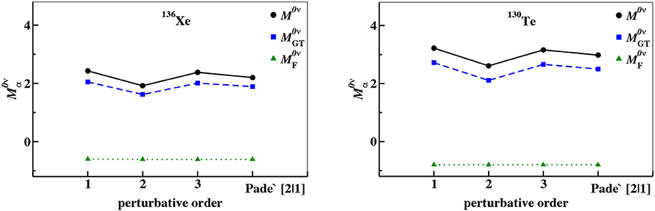
Figure 18. Calculated M^0ν values for the ¹³⁶Xe → ¹³⁶Ba decay (left) and the ¹³⁰Te → ¹³⁰Xe decay (right) as a function of the perturbative order. The green triangles correspond to $M_{F}^{0 ν}$ , the blue squares to $M_{GT}^{0 ν}$ , and the black dots to the full M^0ν. Reproduced from reference [89].

It is worth noting that the perturbative behavior is dominated by the GT component, with the Fermi matrix element $M_{F}^{0 ν}$ being only slightly affected by the renormalization procedure. Moreover, if the order-by-order perturbative behavior of the effective SM 0νββ-decay operator is compared with that of the single β-decay operator, we observe less satisfactory perturbative behavior for the calculation of M^0ν, the difference between the second- and third-order results being about 30% for the ¹³⁰Te and ¹³⁶Xe 0νββ decays.

5. Summary

This paper has presented a general overview of the perturbative approach to deriving effective SM operators, in particular the SM Hamiltonian and decay operators.

First, we described the theoretical framework, which is essentially based on the perturbative expansion of a vertex function—the $\hat{Q}$ -box for the effective Hamiltonian and the $\hat{Θ}$ -box for effective decay operators—whose calculation is pivotal in the Lee-Suzuki similarity transformation. The iterative procedures used to solve the recursive equations that yield effective SM Hamiltonians have been presented in detail, along with tips that could be helpful for calculating the Goldstone diagrams that arise in the perturbative expansion of the above-mentioned vertex functions.

We then reported results from an SM study carried out using only single-particle energies, two-body matrix elements of the residual interaction, and effective decay operators derived from a realistic nuclear potential, without any empirical adjustments. This forms part of a large body of investigations that aim to assess the relevance of such an approach to the study of nuclear structure. The versatility of SM calculations comes from their ability to reproduce experimental results for mass regions ranging from light nuclei (⁴He core [23, 52]) to heavy mass systems (nuclei around ¹³²Sn [121]), as well as to describe exotic and rare phenomena, such as the Borromean structure [124], quadrupole collectivity [98, 100], and the double-β decay process [89, 101, 102] without resorting to empirical adjustments of data.

The results presented in this article testify to the flexibility and usefulness of this theoretical tool, and could provide inspiration for further investigations in the future.

Author Contributions

All authors listed have made a substantial, direct and intellectual contribution to the work, and approved it for publication.

Conflict of Interest

The authors declare that the research was conducted in the absence of any commercial or financial relationships that could be construed as a potential conflict of interest.

References

1. Elliott JP. Nuclear forces and the structure of nuclei. In: Jean M, editor. Cargése Lectures in Physics, Vol. 3. New York, NY: Gordon and Breach (1969). p. 337.

Google Scholar

2. Talmi I. Fifty years of the shell model–the quest for the effective interaction. Adv Nucl Phys. (2003) 27:1. doi: 10.1007/0-306-47916-8_1

CrossRef Full Text | Google Scholar

3. Caurier E, Martínez-Pinedo G, Nowacki F, Poves A, Zuker AP. The shell model as a unified view of nuclear structure. Rev Mod Phys. (2005) 77:427–88. doi: 10.1103/RevModPhys.77.427

CrossRef Full Text | Google Scholar

4. Stroberg SR, Hergert H, Bogner SK, Holt JD. Nonempirical interactions for the nuclear shell model: an update. Annu Rev Nucl Part Sci. (2019) 69:307–62. doi: 10.1146/annurev-nucl-101917-021120

CrossRef Full Text | Google Scholar

5. Kuo TTS, Osnes E. Lecture Notes in Physics. Vol. 364. Berlin: Springer-Verlag (1990).

6. Hjorth-Jensen M, Kuo TTS, Osnes E. Realistic effective interactions for nuclear systems. Phys Rep. (1995) 261:125. doi: 10.1016/0370-1573(95)00012-6

PubMed Abstract | CrossRef Full Text | Google Scholar

7. Coraggio L, Covello A, Gargano A, Itaco N, Kuo TTS. Shell-model calculations and realistic effective interactions. Prog Part Nucl Phys. (2009) 62:135. doi: 10.1016/j.ppnp.2008.06.001

CrossRef Full Text | Google Scholar

8. Bertsch GF. Role of core polarization in two-body interaction. Nucl Phys. (1965) 74:234. doi: 10.1016/0029-5582(65)90262-2

CrossRef Full Text | Google Scholar

9. Kallio A, Kolltveit K. An application of the separation method in shell-model calculation. Nucl Phys. (1964) 53:87. doi: 10.1016/0029-5582(64)90588-7

CrossRef Full Text | Google Scholar

10. Kuo TTS, Brown GE. Structure of finite nuclei and the free nucleon-nucleon interaction: an application to ¹⁸O and ¹⁸F. Nucl Phys. (1966) 85:40. doi: 10.1016/0029-5582(66)90131-3

CrossRef Full Text | Google Scholar

11. Hamada T, Johnston ID. A potential model representation of two-nucleon data below 315 MeV. Nucl Phys. (1962) 34:382. doi: 10.1016/0029-5582(62)90228-6

CrossRef Full Text | Google Scholar

12. Kuo TTS, Brown GE. Reaction matrix elements for the 0f-1p shell nuclei. Nucl Phys A. (1968) 114:241. doi: 10.1016/0375-9474(68)90353-9

CrossRef Full Text | Google Scholar

13. Brown BA, Wildenthal BH. Status of the nuclear shell model. Annu Rev Nucl Part Sci. (1988) 38:29. doi: 10.1146/annurev.ns.38.120188.000333

CrossRef Full Text | Google Scholar

14. Poves A, Sánchez-Solano J, Caurier E, Nowacki F. Shell model study of the isobaric chains A = 50, A = 51 and A = 52. Nucl Phys A. (2001) 694:157. doi: 10.1016/S0375-9474(01)00967-8

CrossRef Full Text | Google Scholar

15. Brandow BH. Linked-cluster expansions for the nuclear many-body problem. Rev Mod Phys. (1967) 39:771. doi: 10.1103/RevModPhys.39.771

CrossRef Full Text | Google Scholar

16. Kuo TTS, Lee SY, Ratcliff KF. A folded-diagram expansion of the model-space effective Hamiltonian. Nucl Phys A. (1971) 176:65. doi: 10.1016/0375-9474(71)90731-7

CrossRef Full Text | Google Scholar

17. Suzuki K, Lee SY. Convergent theory for effective interaction in nuclei. Prog Theor Phys. (1980) 64:2091. doi: 10.1143/PTP.64.2091

CrossRef Full Text | Google Scholar

18. Suzuki K, Okamoto R. Effective operators in time-independent approach. Prog Theor Phys. (1995) 93:905. doi: 10.1143/ptp/93.5.905

CrossRef Full Text | Google Scholar

19. Lee SY, Suzuki K. The effective interaction of two nucleons in the sd shell. Phys Lett B. (1980) 91:173. doi: 10.1016/0370-2693(80)90423-2

CrossRef Full Text | Google Scholar

20. Mayer MG. On closed shells in nuclei. II. Phys Rev. (1949) 75:1969–70. doi: 10.1103/PhysRev.75.1969

CrossRef Full Text | Google Scholar

21. Haxel O, Jensen JHD, Suess HE. On the “magic numbers” in nuclear structure. Phys Rev. (1949) 75:1766. doi: 10.1103/PhysRev.75.1766.2

CrossRef Full Text | Google Scholar

22. Mayer MG, Jensen JHD. Elementary Theory of Nuclear Shell Structure. New York, NY: John Wiley (1955).

Google Scholar

23. Fukui T, De Angelis L, Ma YZ, Coraggio L, Gargano A, Itaco N, et al. Realistic shell-model calculations for p-shell nuclei including contributions of a chiral three-body force. Phys Rev C. (2018) 98:044305. doi: 10.1103/PhysRevC.98.044305

CrossRef Full Text | Google Scholar

24. Ma YZ, Coraggio L, De Angelis L, Fukui T, Gargano A, Itaco N, et al. Contribution of chiral three-body forces to the monopole component of the effective shell-model Hamiltonian. Phys Rev C. (2019) 100:034324. doi: 10.1103/PhysRevC.100.034324

CrossRef Full Text | Google Scholar

25. Brown BA. The nuclear shell model towards the drip lines. Prog Part Nucl Phys. (2001) 47:517. doi: 10.1016/S0146-6410(01)00159-4

CrossRef Full Text | Google Scholar

26. Alex Brown B. The nuclear configuration interations method. In: García-Ramos JE, Andrés MV, Valera JAL, Moro AM, Pérez-Bernal F, editors. Basic Concepts in Nuclear Physics: Theory, Experiments and Applications. RABIDA 2018. Cham: Springer International Publishing (2019). p. 3–31. doi: 10.1007/978-3-030-22204-8_1

PubMed Abstract | CrossRef Full Text | Google Scholar

27. Otsuka T, Gade A, Sorlin O, Suzuki T, Utsuno Y. Evolution of shell structure in exotic nuclei. Rev Mod Phys. (2020) 92:015002. doi: 10.1103/RevModPhys.92.015002

CrossRef Full Text | Google Scholar

28. Morris TD, Parzuchowski NM, Bogner SK. Magnus expansion and in-medium similarity renormalization group. Phys Rev C. (2015) 92:034331. doi: 10.1103/PhysRevC.92.034331

CrossRef Full Text | Google Scholar

29. Sun ZH, Morris TD, Hagen G, Jansen GR, Papenbrock T. Shell-model coupled-cluster method for open-shell nuclei. Phys Rev C. (2018) 98:054320. doi: 10.1103/PhysRevC.98.054320

CrossRef Full Text | Google Scholar

30. Lisetskiy AF, Barrett BR, Kruse MKG, Navratil P, Stetcu I, Vary JP. Ab-initio shell model with a core. Phys Rev C. (2008) 78:044302. doi: 10.1103/PhysRevC.78.044302

CrossRef Full Text | Google Scholar

31. Lisetskiy AF, Kruse MKG, Barrett BR, Navratil P, Stetcu I, Vary JP. Effective operators from exact many-body renormalization. Phys Rev C. (2009) 80:024315. doi: 10.1103/PhysRevC.80.024315

CrossRef Full Text | Google Scholar

32. Dikmen E, Lisetskiy AF, Barrett BR, Maris P, Shirokov AM, Vary JP. Ab initio effective interactions for sd-shell valence nucleons. Phys Rev C. (2015) 91:064301. doi: 10.1103/PhysRevC.91.064301

CrossRef Full Text | Google Scholar

33. Smirnova NA, Barrett BR, Kim Y, Shin IJ, Shirokov AM, Dikmen E, et al. Effective interactions in the sd shell. Phys Rev C. (2019) 100:054329. doi: 10.1103/PhysRevC.100.054329

CrossRef Full Text | Google Scholar

34. Haxton WC, Song CL. Morphing the ShellModel into an effective theory. Phys Rev Lett. (2000) 84:5484–7. doi: 10.1103/PhysRevLett.84.5484

PubMed Abstract | CrossRef Full Text | Google Scholar

35. Kümmel H, Lührmann KH, Zabolitzky JG. Many-fermion theory in expS- (or coupled cluster) form. Phys Rep. (1978) 36:1. doi: 10.1016/0370-1573(78)90081-9

CrossRef Full Text | Google Scholar

36. Schucan TH, Weidenmüller HA. The effective interaction in nuclei and its perturbation expansion: an algebraic approach. Ann Phys. (1972) 73:108. doi: 10.1016/0003-4916(72)90315-6

CrossRef Full Text | Google Scholar

37. Schucan TH, Weidenmüller HA. Perturbation theory for the effective interaction in nuclei. Ann Phys. (1973) 76:483. doi: 10.1016/0003-4916(73)90044-4

CrossRef Full Text | Google Scholar

38. Krenciglowa EM, Kuo TTS. Convergence of effective Hamiltonian expansion and partial summations of folded diagrams. Nucl Phys A. (1974) 235:171. doi: 10.1016/0375-9474(74)90184-5

CrossRef Full Text | Google Scholar

39. Kuo TTS, Krmpotić F, Suzuki K, Okamoto R. Summation of time-dependent folded diagrams for effective interactions with a non-degenerate model space. Nucl Phys A. (1995) 582:205. doi: 10.1016/0375-9474(94)00456-W

CrossRef Full Text | Google Scholar

40. Coraggio L, Itaco N. Self-consistent nuclear shell-model calculation starting from a realistic NN potential. Phys Lett B. (2005) 616:43. doi: 10.1016/j.physletb.2005.04.060

CrossRef Full Text | Google Scholar

41. Takayanagi K. Effective interaction in non-degenerate model space. Nucl Phys A. (2011) 852:61–81. doi: 10.1016/j.nuclphysa.2011.01.003

CrossRef Full Text | Google Scholar

42. Suzuki K, Okamoto R, Kumagai H, Fujii S. Graphical method for deriving an effective interaction with a new vertex function. Phys Rev C. (2011) 83:024304. doi: 10.1103/PhysRevC.83.024304

CrossRef Full Text | Google Scholar

43. Takayanagi K. Effective Hamiltonian in the extended Krenciglowa−Kuo method. Nucl Phys A. (2011) 864:91–112. doi: 10.1016/j.nuclphysa.2011.06.025

CrossRef Full Text | Google Scholar

44. Bloch C, Horowitz J. Sur la détermination des premiers états d'un systéme de fermions dans le cas dégénéré. Nucl Phys. (1958) 8:91. doi: 10.1016/0029-5582(58)90136-6

CrossRef Full Text | Google Scholar

45. Tsunoda N, Takayanagi K, Hjorth-Jensen M, Otsuka T. Multi-shell effective interactions. Phys Rev C. (2014) 89:024313. doi: 10.1103/PhysRevC.89.024313

CrossRef Full Text | Google Scholar

46. Tsunoda N, Otsuka T, Shimizu N, Hjorth-Jensen M, Takayanagi K, Suzuki T. Exotic neutron-rich medium-mass nuclei with realistic nuclear forces. Phys Rev C. (2017) 95:021304. doi: 10.1103/PhysRevC.95.021304

CrossRef Full Text | Google Scholar

47. Sun ZH, Wu Q, Zhao ZH, Hu BS, Dai SJ, Xu FR. Resonance and continuum Gamow shell model with realistic nuclear forces. Phys Lett B. (2017) 769:227–32. doi: 10.1016/j.physletb.2017.03.054

CrossRef Full Text | Google Scholar

48. Ma YZ, Xu FR, Coraggio L, Hu BS, Li JG, Fukui T, et al. Chiral three-nucleon force and continuum for dripline nuclei and beyond. Phys Lett B. (2020) 802:135257. doi: 10.1016/j.physletb.2020.135257

CrossRef Full Text | Google Scholar

49. Press WH, Teukolsky SA, Vetterling WT, Flannery BP. Fortran Numerical Recipes. Vol. 1. Cambridge: Cambridge University Press (1992).

Google Scholar

50. Shurpin J, Kuo TTS, Strottman D. Folded diagrams and 1s-0d effective interactions derived from Reid and Paris nucleon-nucleon potentials. Nucl Phys A. (1983) 408:310. doi: 10.1016/0375-9474(83)90586-9

CrossRef Full Text | Google Scholar

51. Kuo TTS, Shurpin J, Tam KC, Osnes E, Ellis PJ. A simple method for evaluating Goldstone diagrams in an angular momentum coupled representation. Ann Phys. (1981) 132:237. doi: 10.1016/0003-4916(81)90068-3

CrossRef Full Text | Google Scholar

52. Coraggio L, Covello A, Gargano A, Itaco N, Kuo TTS. Effective shell-model hamiltonians from realistic nucleon-nucleon potentials within a perturbative approach. Ann Phys. (2012) 327:2125. doi: 10.1016/j.aop.2012.04.013

CrossRef Full Text | Google Scholar

53. Paldus J, Wong HC. Computer generation of Feynman diagrams for perturbation theory I. General algorithm. Comput Phys Commun. (1973) 6:1–7. doi: 10.1016/0010-4655(73)90016-7

CrossRef Full Text | Google Scholar

54. Edmonds AR. Angular Momentum in Quantum Mechanics. Princeton, NJ: Princeton University Press (1957).

Google Scholar

55. Johnson CW, Ormand WE, Krastev PG. Factorization in large-scale many-body calculations. Comput Phys Commun. (2013) 184:2761–74. doi: 10.1016/j.cpc.2013.07.022

CrossRef Full Text | Google Scholar

56. Hjorth-Jensen M, Lombardo MP, van Kolck U, editors. Lecture Notes in Physics. Vol. 936. Berlin: Springer (2017).

Google Scholar

57. Polls A, Müther H, Faessler A, Kuo TTS, Osnes E. Three-body forces in sd-shell nuclei. Nucl Phys A. (1983) 401:124. doi: 10.1016/0375-9474(83)90340-8

CrossRef Full Text | Google Scholar

58. Ellis PJ, Osnes E. An introductory guide to effective operators in nuclei. Rev Mod Phys. (1977) 49:777. doi: 10.1103/RevModPhys.49.777

CrossRef Full Text | Google Scholar

59. Mavromatis HA, Zamick L, Brown GE. First and second order corrections to the magnetic moments of nuclei using realistic interactions. Nucl Phys. (1966) 80:545–64. doi: 10.1016/0029-5582(66)90063-0

CrossRef Full Text | Google Scholar

60. Mavromatis HA, Zamick L. Magnetic moments of nuclei with closed j-j shells plus or minus one nucleon. Nucl Phys A. (1967) 104:17–34. doi: 10.1016/0375-9474(67)90754-3

CrossRef Full Text | Google Scholar

61. Federman P, Zamick L. State-dependent effective charge in the 2p−1f shell. Phys Rev. (1969) 177:1534–40. doi: 10.1103/PhysRev.177.1534

CrossRef Full Text | Google Scholar

62. Towner IS, Khanna KFC. Corrections to the single-particle M1 and Gamow−Teller matrix elements. Nucl Phys A. (1983) 399:334. doi: 10.1016/0375-9474(83)90252-X

CrossRef Full Text | Google Scholar

63. Towner IS. Quenching of spin matrix elements in nuclei. Phys Rep. (1987) 155:263. doi: 10.1016/0370-1573(87)90138-4

CrossRef Full Text | Google Scholar

64. Avignone FT, Elliott SR, Engel J. Double beta decay, Majorana neutrinos, and neutrino mass. Rev Mod Phys. (2008) 80:481–516. doi: 10.1103/RevModPhys.80.481

CrossRef Full Text | Google Scholar

65. Vergados JD, Ejiri H, Šimkovic F. Theory of neutrinoless double beta decay. Rep Prog Phys. (2012) 75:106301. doi: 10.1088/0034-4885/75/10/106301

PubMed Abstract | CrossRef Full Text | Google Scholar

66. Kotila J, Iachello F. Phase-space factors for double-β decay. Phys Rev C. (2012) 85:034316. doi: 10.1103/PhysRevC.85.034316

PubMed Abstract | CrossRef Full Text | Google Scholar

67. Stoica S, Mirea M. New calculations for phase space factors involved in double-β decay. Phys Rev C. (2013) 88:037303. doi: 10.1103/PhysRevC.88.037303

CrossRef Full Text | Google Scholar

68. Barea J, Iachello F. Neutrinoless double-β decay in the microscopic interacting boson model. Phys Rev C. (2009) 79:044301. doi: 10.1103/PhysRevC.79.044301

CrossRef Full Text | Google Scholar

69. Barea J, Kotila J, Iachello F. Limits on neutrino masses from neutrinoless double-β decay. Phys Rev Lett. (2012) 109:042501. doi: 10.1103/PhysRevLett.109.042501

PubMed Abstract | CrossRef Full Text | Google Scholar

70. Barea J, Kotila J, Iachello F. Nuclear matrix elements for double-β decay. Phys Rev C. (2013) 87:014315. doi: 10.1103/PhysRevC.87.014315

CrossRef Full Text | Google Scholar

71. Šimkovic F, Faessler A, Rodin V, Vogel P, Engel J. Anatomy of the 0νββ nuclear matrix elements. Phys Rev C. (2008) 77:045503. doi: 10.1103/PhysRevC.77.045503

CrossRef Full Text | Google Scholar

72. Šimkovic F, Faessler A, Müther H, Rodin V, Stauf M. 0νββ-decay nuclear matrix elements with self-consistent short-range correlations. Phys Rev C. (2009) 79:055501. doi: 10.1103/PhysRevC.79.055501

CrossRef Full Text | Google Scholar

73. Fang DL, Faessler A, Rodin V, Šimkovic F. Neutrinoless double-β decay of deformed nuclei within quasiparticle random-phase approximation with a realistic interaction. Phys Rev C. (2011) 83:034320. doi: 10.1103/PhysRevC.83.034320

CrossRef Full Text | Google Scholar

74. Faessler A, Rodin V, Simkovic F. Nuclear matrix elements for neutrinoless double-beta decay and double-electron capture. J Phys G. (2012) 39:124006. doi: 10.1088/0954-3899/39/12/124006

CrossRef Full Text | Google Scholar

75. Rodríguez TR, Martínez-Pinedo G. Energy density functional study of nuclear matrix elements for neutrinoless ββ decay. Phys Rev Lett. (2010) 105:252503. doi: 10.1103/PhysRevLett.105.252503

PubMed Abstract | CrossRef Full Text | Google Scholar

76. Song LS, Yao JM, Ring P, Meng J. Relativistic description of nuclear matrix elements in neutrinoless double-β decay. Phys Rev C. (2014) 90:054309. doi: 10.1103/PhysRevC.90.054309

CrossRef Full Text | Google Scholar

77. Yao JM, Song LS, Hagino K, Ring P, Meng J. Systematic study of nuclear matrix elements in neutrinoless double-β decay with a beyond-mean-field covariant density functional theory. Phys Rev C. (2015) 91:024316. doi: 10.1103/PhysRevC.91.024316

CrossRef Full Text | Google Scholar

78. Song LS, Yao JM, Ring P, Meng J. Nuclear matrix element of neutrinoless double-β decay: relativity and short-range correlations. Phys Rev C. (2017) 95:024305. doi: 10.1103/PhysRevC.95.024305

CrossRef Full Text | Google Scholar

79. Jiao CF, Engel J, Holt JD. Neutrinoless double-β decay matrix elements in large shell-model spaces with the generator-coordinate method. Phys Rev C. (2017) 96:054310. doi: 10.1103/PhysRevC.96.054310

CrossRef Full Text | Google Scholar

80. Yao JM, Engel J, Wang LJ, Jiao CF, Hergert H. Generator-coordinate reference states for spectra and 0νββ decay in the in-medium similarity renormalization group. Phys Rev C. (2018) 98:054311. doi: 10.1103/PhysRevC.98.054311

CrossRef Full Text | Google Scholar

81. Jiao CF, Horoi M, Neacsu A. Neutrinoless double-β decay of ¹²⁴Sn, ¹³⁰Te, and ¹³⁶Xe in the Hamiltonian-based generator-coordinate method. Phys Rev C. (2018) 98:064324. doi: 10.1103/PhysRevC.98.064324

CrossRef Full Text | Google Scholar

82. Jiao C, Johnson CW. Union of rotational and vibrational modes in generator-coordinate-type calculations, with application to neutrinoless double-β decay. Phys Rev C. (2019) 100:031303. doi: 10.1103/PhysRevC.100.031303

CrossRef Full Text | Google Scholar

83. Menéndez J, Poves A, Caurier E, Nowacki F. Occupancies of individual orbits, and the nuclear matrix element of the ⁷⁶Ge neutrinoless ββ decay. Phys Rev C. (2009) 80:048501. doi: 10.1103/PhysRevC.80.048501

CrossRef Full Text | Google Scholar

84. Menéndez J, Poves A, Caurier E, Nowacki F. Disassembling the nuclear matrix elements of the neutrinoless ββ decay. Nucl Phys A. (2009) 818:139. doi: 10.1016/j.nuclphysa.2008.12.005

CrossRef Full Text | Google Scholar

85. Horoi M, Brown BA. Shell-model analysis of the ¹³⁶Xe double beta decay nuclear matrix elements. Phys Rev Lett. (2013) 110:222502. doi: 10.1103/PhysRevLett.110.222502

PubMed Abstract | CrossRef Full Text | Google Scholar

86. Neacsu A, Horoi M. Shell model studies of the ¹³⁰Te neutrinoless double-β decay. Phys Rev C. (2015) 91:024309. doi: 10.1103/PhysRevC.91.024309

CrossRef Full Text | Google Scholar

87. Brown BA, Fang DL, Horoi M. Evaluation of the theoretical nuclear matrix elements for ββ decay of ⁷⁶Ge. Phys Rev C. (2015) 92:041301. doi: 10.1103/PhysRevC.92.041301

CrossRef Full Text | Google Scholar

88. Engel J, Menéndez J. Status and future of nuclear matrix elements for neutrinoless double-beta decay: a review. Rep Prog Phys. (2017) 80:046301. doi: 10.1088/1361-6633/aa5bc5

PubMed Abstract | CrossRef Full Text | Google Scholar

89. Coraggio L, Gargano A, Itaco N, Mancino R, Nowacki F. Calculation of the neutrinoless double-β decay matrix element within the realistic shell model. Phys Rev C. (2020) 101:044315. doi: 10.1103/PhysRevC.101.044315

CrossRef Full Text | Google Scholar

90. Machleidt R. High-precision, charge-dependent Bonn nucleon-nucleon potential. Phys Rev C. (2001) 63:024001. doi: 10.1103/PhysRevC.63.024001

CrossRef Full Text | Google Scholar

91. Song HQ, Wu HF, Kuo TTS. Effect of nuclear core polarization on neutrinoless double beta decay of ⁴⁸Ca. Phys Rev C. (1989) 40:2260–4. doi: 10.1103/PhysRevC.40.2260

PubMed Abstract | CrossRef Full Text | Google Scholar

92. Staudt A, Kuo TTS, Klapdor-Kleingrothaus HV. ββ decay of ¹²⁸Te, ¹³⁰Te, and ⁷⁶Ge with renormalized effective interactions derived from Paris and Bonn potentials. Phys Rev C. (1992) 46:871–83. doi: 10.1103/PhysRevC.46.871

PubMed Abstract | CrossRef Full Text | Google Scholar

93. Holt JD, Engel J. Effective double-β-decay operator for ⁷⁶Ge and ⁸²Se. Phys Rev C. (2013) 87:064315. doi: 10.1103/PhysRevC.87.064315

CrossRef Full Text | Google Scholar

94. Alfonso K, Artusa DR, Avignone FT, Azzolini O, Balata M, Banks TI, et al. Search for neutrinoless double-beta decay of ¹³⁰Te with CUORE − 0. Phys Rev Lett. (2015) 115:102502. doi: 10.1103/PhysRevLett.115.102502

PubMed Abstract | CrossRef Full Text | Google Scholar

95. Auger M, Auty DJ, Barbeau PS, Beauchamp E, Belov V, Benitez-Medina C, et al. Search for neutrinoless double-beta decay in ¹³⁶Xe with EXO − 200. Phys Rev Lett. (2012) 109:032505. doi: 10.1103/PhysRevLett.109.032505

PubMed Abstract | CrossRef Full Text | Google Scholar

96. Gando A, Gando Y, Hachiya T, Hayashi A, Hayashida S, Ikeda H, et al. Search for Majorana neutrinos near the inverted mass hierarchy region with KamLAND−Zen. Phys Rev Lett. (2016) 117:082503. doi: 10.1103/PhysRevLett.117.082503

CrossRef Full Text | Google Scholar

97. Bogner S, Kuo TTS, Coraggio L, Covello A, Itaco N. Low momentum nucleon-nucleon potential and shell model effective interactions. Phys Rev C. (2002) 65:051301(R). doi: 10.1103/PhysRevC.65.051301

CrossRef Full Text | Google Scholar

98. Coraggio L, Covello A, Gargano A, Itaco N, Kuo TTS. Shell-model study of quadrupole collectivity in light tin isotopes. Phys Rev C. (2015) 91:041301. doi: 10.1103/PhysRevC.91.041301

CrossRef Full Text | Google Scholar

99. Coraggio L, Gargano A, Itaco N. Role of three-nucleon forces in neutron-rich nuclei beyond ¹³²Sn. JPS Conf Proc. (2015) 6:020046. doi: 10.7566/JPSCP.6.020046

CrossRef Full Text | Google Scholar

100. Coraggio L, Gargano A, Itaco N. Double-step truncation procedure for large-scale shell-model calculations. Phys Rev C. (2016) 93:064328. doi: 10.1103/PhysRevC.93.064328

CrossRef Full Text | Google Scholar

101. Coraggio L, De Angelis L, Fukui T, Gargano A, Itaco N. Calculation of Gamow−Teller and two-neutrino double-β decay properties for ¹³⁰Te and ¹³⁶Xe with a realistic nucleon-nucleon potential. Phys Rev C. (2017) 95:064324. doi: 10.1103/PhysRevC.95.064324

CrossRef Full Text | Google Scholar

102. Coraggio L, De Angelis L, Fukui T, Gargano A, Itaco N, Nowacki F. Renormalization of the Gamow − Teller operator within the realistic shell model. Phys Rev C. (2019) 100:014316. doi: 10.1103/PhysRevC.100.014316

CrossRef Full Text | Google Scholar

103. Data extracted using the NNDC On-line Data Service from the ENSDF database, file revised as of April 3, 2020 (2020).

Google Scholar

104. Data extracted using the NNDC On-line Data Service from the XUNDL database, file revised as of April 6, 2020 (2020).

Google Scholar

105. Goodman CD, Goulding CA, Greenfield MB, Rapaport J, Bainum DE, Foster CC, et al. Gamow − Teller matrix elements from 0° (p, n) cross sections. Phys Rev Lett. (1980) 44:1755–9. doi: 10.1103/PhysRevLett.44.1755

CrossRef Full Text | Google Scholar

106. Taddeucci TN, Goulding CA, Carey TA, Byrd RC, Goodman CD, Gaarde C, et al. The (p, n) reaction as a probe of beta decay strength. Nucl Phys A. (1987) 469:125. doi: 10.1016/0375-9474(87)90089-3

CrossRef Full Text | Google Scholar

107. Puppe P, Lennarz A, Adachi T, Akimune H, Ejiri H, Frekers D, et al. High resolution (³He,t) experiment on the double-β decaying nuclei ¹²⁸Te and ¹³⁰Te. Phys Rev C. (2012) 86:044603. doi: 10.1103/PhysRevC.86.044603

CrossRef Full Text | Google Scholar

108. Frekers D, Puppe P, Thies JH, Ejiri H. Gamow − Teller strength extraction from (³He,t) reactions. Nucl Phys A. (2013) 916:219. doi: 10.1016/j.nuclphysa.2013.08.006

CrossRef Full Text | Google Scholar

109. Barabash AS. Average and recommended half-life values for two-neutrino double beta decay. Nucl Phys A. (2015) 935:52. doi: 10.1016/j.nuclphysa.2015.01.001

CrossRef Full Text | Google Scholar

110. Caurier E, Nowacki F, Poves A. Shell model description of the ββ decay of ¹³⁶Xe. Phys Lett B. (2012) 711:62. doi: 10.1016/j.physletb.2012.03.076

CrossRef Full Text | Google Scholar

111. Haxton WC, Stephenson GJ Jr. Double beta decay. Prog Part Nucl Phys. (1984) 12:409. doi: 10.1016/0146-6410(84)90006-1

CrossRef Full Text | Google Scholar

112. Tomoda T. Double beta decay. Rep Prog Phys. (1991) 54:53. doi: 10.1088/0034-4885/54/1/002

CrossRef Full Text | Google Scholar

113. Park TS, Min DP, Rho M. Chiral dynamics and heavy-fermion formalism in nuclei: exchange axial currents. Phys Rep. (1993) 233:341. doi: 10.1016/0370-1573(93)90099-Y

CrossRef Full Text | Google Scholar

114. Pastore S, Girlanda L, Schiavilla R, Viviani M, Wiringa RB. Electromagnetic currents and magnetic moments in chiral effective field theory (χEFT). Phys Rev C. (2009) 80:034004. doi: 10.1103/PhysRevC.80.034004

CrossRef Full Text | Google Scholar

115. Piarulli M, Girlanda L, Marcucci LE, Pastore S, Schiavilla R, Viviani M. Electromagnetic structure of A = 2 and 3 nuclei in chiral effective field theory. Phys Rev C. (2013) 87:014006. doi: 10.1103/PhysRevC.87.014006

CrossRef Full Text | Google Scholar

116. Pastore S, Carlson J, Cirigliano V, Dekens W, Mereghetti E, Wiringa RB. Neutrinoless double-β decay matrix elements in light nuclei. Phys Rev C. (2018) 97:014606. doi: 10.1103/PhysRevC.97.014606

CrossRef Full Text | Google Scholar

117. Coraggio L, Itaco N, Mancino R. Short-range correlations for neutrinoless double-beta decay and low-momentum NN potentials. arXiv. (2019) 191004146[nucl-th].

Google Scholar

118. Tanabashi M, Hagiwara K, Hikasa K, Nakamura K, Sumino Y, Takahashi F, et al. Review of Particle Physics. Phys Rev D. (2018) 98:030001. doi: 10.1103/PhysRevD.98.030001

CrossRef Full Text | Google Scholar

119. Suhonen J. Impact of the quenching of g_A on the sensitivity of 0νββ experiments. Phys Rev C. (2017) 96:055501. doi: 10.1103/PhysRevC.96.055501

CrossRef Full Text | Google Scholar

120. Suhonen JT. Value of the axial-vector coupling strength in β and ββ decays: a review. Front Phys. (2017) 5:55. doi: 10.3389/fphy.2017.00055

CrossRef Full Text | Google Scholar

121. Coraggio L, Covello A, Gargano A, Itaco N, Kuo TTS. Shell-model study of the N = 82 isotonic chain with a realistic effective Hamiltonian. Phys Rev C. (2009) 80:044320. doi: 10.1103/PhysRevC.80.044320

CrossRef Full Text | Google Scholar

122. Coraggio L, De Angelis L, Fukui T, Gargano A, Itaco N. Two-neutrino double-beta decay within the realistic shell model. J Phys Conf Ser. (2018) 1056:012012. doi: 10.1088/1742-6596/1056/1/012012

CrossRef Full Text | Google Scholar

123. Baker GA, Gammel JL. The Padé Approximant in Theoretical Physics. Vol. 71 of Mathematics in Science and Engineering. New York, NY: Academic Press (1970).

Google Scholar

124. Coraggio L, Covello A, Gargano A, Itaco N. Shell-model calculations for neutron-rich carbon isotopes with a chiral nucleon-nucleon potential. Phys Rev C. (2010) 81:064303. doi: 10.1103/PhysRevC.81.064303

CrossRef Full Text | Google Scholar

Keywords: nuclear shell model, effective interactions, many-body perturbation theory, nuclear forces, double-beta decay

Citation: Coraggio L and Itaco N (2020) Perturbative Approach to Effective Shell-Model Hamiltonians and Operators. Front. Phys. 8:345. doi: 10.3389/fphy.2020.00345

Received: 15 May 2020; Accepted: 22 July 2020;
Published: 15 October 2020.

Edited by:

Michele Viviani, National Institute of Nuclear Physics of Pisa, Italy

Reviewed by:

Artur Polls, University of Barcelona, Spain
Daniel Phillips, Ohio University, United States

Copyright © 2020 Coraggio and Itaco. This is an open-access article distributed under the terms of the Creative Commons Attribution License (CC BY). The use, distribution or reproduction in other forums is permitted, provided the original author(s) and the copyright owner(s) are credited and that the original publication in this journal is cited, in accordance with accepted academic practice. No use, distribution or reproduction is permitted which does not comply with these terms.

*Correspondence: Luigi Coraggio, luigi.coraggio@na.infn.it; Nunzio Itaco, nunzio.itaco@unicampania.it

REVIEW article

Perturbative Approach to Effective Shell-Model Hamiltonians and Operators

1. Introduction

2. General Overview

3. Perturbative Expansion of Effective Shell-Model Operators

3.1. The Lee-Suzuki Similarity Transformation

3.1.1. The Krenciglowa-Kuo Iterative Technique

3.1.2. The Lee-Suzuki Iterative Technique

3.1.3. The Kuo-Krenciglowa Technique Extended to Non-degenerate Model Spaces

3.1.4. The $\hat{Z}$ (ϵ) Vertex Function

3.2. Diagrammatic Expansion of the $\hat{Q}$ -box Vertex Function

3.3. Effective Shell-Model Decay Operators

4. Applications

4.1. The Double-β Decay Around Doubly Closed ¹³²Sn

5. Summary

Author Contributions

Conflict of Interest

References

This article is part of the Research Topic

People also looked at

REVIEW article

Perturbative Approach to Effective Shell-Model Hamiltonians and Operators

1. Introduction

2. General Overview

3. Perturbative Expansion of Effective Shell-Model Operators

3.1. The Lee-Suzuki Similarity Transformation

3.1.1. The Krenciglowa-Kuo Iterative Technique

3.1.2. The Lee-Suzuki Iterative Technique

3.1.3. The Kuo-Krenciglowa Technique Extended to Non-degenerate Model Spaces

3.1.4. The Z^(ϵ) Vertex Function

3.2. Diagrammatic Expansion of the Q^-box Vertex Function

3.3. Effective Shell-Model Decay Operators

4. Applications

4.1. The Double-β Decay Around Doubly Closed 132Sn

5. Summary

Author Contributions

Conflict of Interest

References

This article is part of the Research Topic

People also looked at

3.1.4. The $\hat{Z}$ (ϵ) Vertex Function

3.2. Diagrammatic Expansion of the $\hat{Q}$ -box Vertex Function

4.1. The Double-β Decay Around Doubly Closed ¹³²Sn