Low-Field MRI: How Low Can We Go? A Fresh View on an Old Debate

Introduction

Low field MRI? The rationale behind it has been around for quite some time, traditionally perceived as a mean to reduce cost or to provide open access to patients suffering from claustrophobia. Over the past 30 years, scientists have supported low-field MRI on multiple occasions and brought facts that corroborate clinical relevance [1–4]. Yet, low field MRI has not spread. Reasons that have been invoked are diverse and have led to numerous debates. From the manufacturer point-of-view, the current business model in MRI results in higher margins allowing to increase profit [5]. From a clinical and academic point-of-view, the quest for higher and higher spatial resolution has led radiologists and scientists worldwide to always push toward high- and ultra-high field MRI research, eventually dominating over all others in peer reviewed journals [6]. One sure thing is that the statistics of MRI sales over the last two decades have certainly helped closing that debate. Nowadays high-field MRI sales (B₀≥ 1.5 T) represent about 85% of the market size in Europe and North America [7]. One of the main misconceptions is that low-field MRI translates into poor image resolution, often associated with poor image quality. It is important, as scientists, to state that this concept is purely and simply wrong. Magnetic field strength has by no means ever been a limit to an achievable image resolution. A brief jump into the early days of MRI is enough to appreciate the tremendous leap in image quality that was made for a given field strength (Figure 1). More recent work from Choquet et al. [9] has reported MRI of different mouse body parts in vivo at 0.1 T (~4.3 MHz) with down to 100 × 100 × 750 μm³ voxel size, more than 10 years ago (Figure 2). Sensitivity though, and how far the signal lies above the detection chain's noise floor will tell about one's capability to achieve a given resolution in the minimum amount of time. Hence time really is the argument at stake when considering lower field options. Indeed, lower field strengths result in lower bulk magnetization of nuclear spins leading in turn to a reduced sensitivity. Assuming a fixed noise floor in the detection chain, the decreased total magnetic moment brings the maximum signal detectable closer to the latter and the overall signal-to-noise ratio (SNR) drops. One main alternative to compensate for this loss is signal averaging. It is generally accepted that n averages will produce an SNR gain of $\sqrt{n}$. Hence time is currently the true limit to a wide spread of low-field MRI, due to lower overall NMR sensitivity. However, this is also a matter of perspective. Why time considerations have become key in clinical diagnosis has to be contextualized in the current landscape of MRI. Most hospitals currently host one or two MRI scanners, which cost roughly scales with magnetic field (~$1M/T). As such MRI units are expensive and used for the imaging of all body parts, they are likely to represent a bottleneck in clinical workflows. Hence, the time needed for one scan has to be short in order to scan as many patients as possible within a day. Nowadays, no one can afford a machine that would perform slower than the state-of-the art because there is such a high demand for non-invasive radiation-free diagnosis. Yet, other than applications where speed is truly paramount such as for cardiovascular applications, or patients with a life-threatening risk, fast imaging is only required due to scanners being a low-volume/high price equipment. One could argue that this quest for speed is not as relevant if numerous low-field, low-cost devices were to be used (high-volume, low-price). After all, if the price of a scanner is divided by two and the acquisition time multiplied by two, then the cost per unit time stays the same, and the same number of patients can be scanned within the same time slot. Only cost for personnel would increase. The situation in China is a good illustration of this point: the high population density requires a higher density of MR units, and mid-field MR units represent about 50% of the market size [10], vs. 6% in Europe and North America [7]. As a consequence, depending on the market ability to embrace such a change in paradigm, that approach would naturally reduce pressure on acquisition times. Most importantly, rather than acquisition time or image resolution, one key aspect in the democratization of low-field MRI resides in its value. Most likely, if manufacturers and end users would foresee higher value in low-field MRI solutions, there would be a straightforward path toward mass adoption. Value though is a complex concept that finds different resonances across populations and cultures. One should agree on a simple description of value as being the ratio of a benefit over a cost [11]. For low-field technology to be truly visible and adopted, its value in MRI diagnosis would hence need to be increased. Two approaches then allow to increase value; 1-reduce cost, 2-increase benefits, or both at the same time. Considering cost, the last two decades have already shown that relevant diagnosis can be achieved in lower-cost lower-field devices [12–17]. Interest though, is hard to trigger if value increases only slightly and yet no broad adoption has followed since. For example, commercially available low-field scanners rely on permanent magnet technology that can weigh up to 13 tons. Thus, their individual cost (that includes siting) has never reached a point where value goes through the roof and triggers such a cultural change. Maybe the economic pressure on health expenses will change the current landscape with populations worldwide aging and growing, but this has been a long-heard argument never followed by action. Eventually, it appears challenging to spark interest in both radiologists and academics only by lowering cost as this is often perceived as leading to less potent technology, except maybe when the research is directed toward developing countries. The latter field of research is considered a niche though, and if cost is one key to selling in these countries, “low-cost” alone will never replace tailor-made solutions to country-specific needs. The alternative to increased value is then to increase benefits. Nowadays, MRI units require specific siting from their heavy weight and intense magnetic field strength, and shielding from magnetic and electromagnetic disturbances. MRI systems are known to be incompatible with most devices unless they are specifically made MRI-compatible. Increasing accessibility by means of a (much) lower footprint, little siting requirement, or enhanced compatibility certainly is a path toward increased benefits, and hence increased value. Now, what key element is driving such heavy weights, compatibility aspects, and ultimately the cost of MRI machines nowadays? Magnetic field is. As a result, low magnetic field MRI could very likely bring high value from both decreased costs and enhanced benefits. But how low can we go? In this manuscript, we aim to provide a fresh view on this old debate in MRI.

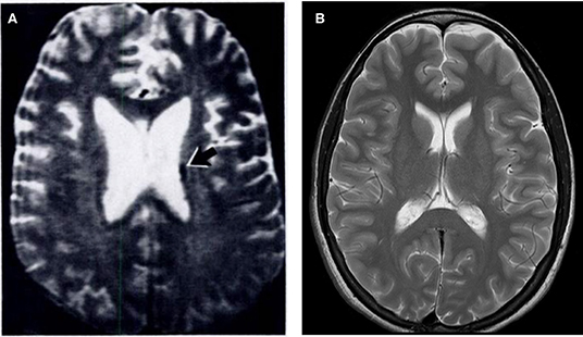
Figure 1. T₂-weighted MR brain images acquired at 1.5 T in (A) 1986. Image reused, with permission, from Zimmerman et al. [8] and (B) 2009 (authors' database).

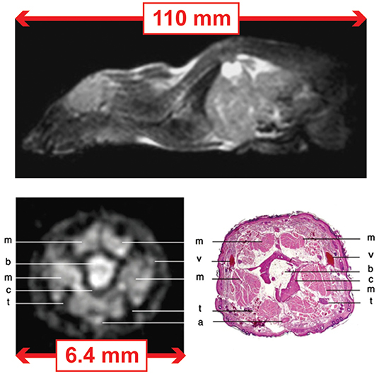
Figure 2. MRI images of the mouse acquired at 0.1 T using a FISP sequence and dedicated coils for the whole-body and tail. (Top) Whole body: field-of-view (FoV) of 110 mm and in plane resolution of 430 × 430 μm². The acquisition time was 30 min for 30 slices of ~1 mm thickness. (Bottom) Tail: field-of-view (FoV) of 6.4 mm and in plane resolution of 100 × 100 μm². The acquisition time was 1 h 30 min for 26 slices of ~ 750 μm thickness. Images modified, with permission, from Choquet et al. [9].

SNR, the Elephant in the Room

SNR indeed, is the elephant in the room when it comes to low-field MRI. Lower Boltzmann distribution infers lower induced voltages in inductive detection that translates into lower signal. A generally accepted assumption is that SNR scales with the static magnetic field $B_0^{\frac{7}{4}}$ for frequencies above 5 MHz, and $B_0^{\frac{3}{2}}$ at low frequencies (below ~5 MHz) [18]. One of the main challenges for low-field MR experts is thus to compensate for the loss in SNR per unit time inherited from the reduced magnetic field. Recent work laid an exhaustive portrait of mid-field MRI in the range 0.25–1 T [19], pointing out the current gain of interest for alternative solutions. Increasing SNR via magnets that are not “too” weak certainly is an approach to preserve signal. The latter has some merit considering the tremendous amount of progress magnetic resonance has benefited from over the last three decades, as illustrated in Figure 1 and in [15]. As a result, most recent developments will translate easily in mid-field regimes which detection physics and design considerations are close to ¹H NMR at most widely spread 1.5 T. That said, the big difference in images obtained between the 80's and today at 1.5 T also highlights how field strength is not a guarantee for good image quality, and how much it has to be balanced with high performance acquisition techniques, high sensitivity detectors, image processing, and modern electronics all combined together. Another comment on medium range 0.25–1 T MRI is that it might not allow to move sufficiently far from typical constraints found in high-field MRI. Among them, exclusive magnets made of superconductors for fields higher than 0.5 T [19], magnet weight, low tolerance to magnetic environments and magnetic susceptibility effects. One should keep in mind that an interesting approach to tame SNR is favoring regimes sufficiently different from inductive detection passed 15 MHz, with a focus on noise considerations. As an example, noise predominance below 5 MHz for a variety of coil sizes comes from the coil when body noise predominance is the general rule in mainstream high-field MRI [20]. Current acceleration methods for clinical MR imaging such as parallel imaging are even dictated by sample noise predominance as each coil sees coherent noise from the sample. In the present manuscript, in order to complement existing review work and report on the latest and most active low and ultra-low field MRI research, the authors have narrowed down the span of low-field MRI research considered to articles published within the past 5 years at field < 0.2 T (< 8.5 MHz). More specifically, the authors are reporting on work that already have produced images (even if not yet clinically relevant or only in phantoms), yet excluding simulated work.

Hardware Considerations

Magnets

The MRI community shows a growing interest for small footprint MRI technology leveraging low-magnetic fields. Worldwide, an effort has started to spread from hardware and engineering considerations, notably regarding magnet construction.

Permanent Magnets

One of the main clinical application envisioned for small footprint, point-of-care MRI is neuroimaging. Many academic sites driving this effort have opted for permanent magnet architectures, for the most part deriving designs from recent work making use of Halbach geometries [21]. Permanent magnets are of particular interest because they do not require power to produce the spin-polarizing static magnetic field B₀. Zimmerman-Cooley et al. [21] have reported on two generations of lightweight magnets. The first generation uses the intrinsic inhomogeneity found in Halbach magnet geometries for spatial encoding, whereas the second version features a constant 1D spatial encoding magnetic field gradient (SEM) superimposed on the static magnetic field B₀ [22]. In this second iteration, 2D encoding is obtained either by physically rotating the native 1D SEM around the object of interest, or by using a custom made gradient insert avoiding physical rotation [22]. Three-dimensional encoding is obtained from the same gradient insert, from an additional coil arrangement in the last spatial direction. The magnet features a 29-cm diameter bore and weighs 122 kg for an average B₀ of 79.3 mT (3.4 MHz). Field homogeneity is 27,800 ppm (~95 kHz) over a 20-cm diameter spherical volume (DSV). Imaging capability is still in its infancy but several promising approaches are being assessed. Recent work from O'Reilly et al. [23] similarly report on a 27-cm diameter bore Halbach array magnet construction. The latter proposes a classic approach to magnet design used at high-field, where the static magnetic field homogeneity is being optimized first, and complemented by a gradient insert featuring coils for spatial encoding in 3 dimensions. The presented magnet weighs ~75 kg for an average magnetic field of 50.4 mT (2.15 MHz). The measured magnetic field shows ~2,500 ppm (~5 kHz) homogeneity across a 20-cm DSV. Pushing toward more compact designs, McDaniel et al. [24] have designed and built a head-size, hemispheric magnet consisting of an assembly of NdFeB blocks inserted into a 3D printed former. The magnet weighs 6.3 kg with a mean B₀ of 63.6 mT (2.67 MHz). Over the targeted ROI of ~3 × 8 × 8 cm³, B₀ covers a 69,200 ppm (~190 kHz) range. The magnet was designed with a built-in field gradient of ~117 mT/m. For the remaining spatial encoding directions, two single-sided, hemispherically-shaped gradient coils were wound on the outside of the magnet former. Further away from applications in vivo, yet with a major emphasis on portability and democratization of MR technology, Greer et al. [25] have presented a hand-held MR system for 2D imaging (projection) in ~9-mm diameter objects using permanent magnets arranged in a curved single-sided geometry. This device follows the steps of the previously released NMR-MOUSE [26, 27]. After numerical optimization, five NdFeB magnets are arranged so that the sample of interest is partially enclosed by the magnet, allowing to obtain a higher B₀ of 186 mT (8 MHz). The 2D field of view is 9 × 9 mm² with ~58,500 ppm homogeneity (~460 kHz) over a 5-mm depth (G₀ = 2, 200 mT/m). The system features two planar gradients coils printed on PCB. The typical pitfalls for permanent magnet constructions rely in the magnetic field being constantly turned-on, weight, important field inhomogeneity, and poor temperature stability. Weight can be mitigated in purpose-built small size scanner, yet temperature can yield several kilohertz frequency shifts per degree caused both by environmental changes and heating from other components of the scanner, such as gradient coils. Strategies to regulate magnet temperature or to account for resulting frequency drifts in imaging or post-processing pipelines will be crucially needed in order for these technologies to be democratized.

Electromagnets

Electromagnets are an equally relevant alternative for low-field MRI, generally providing better field homogeneity than permanent magnets. In terms of flexibility, they can be turned on and off at will, and the generated field can be modulated by varying the input current in the magnet coils. Electromagnets operating at low field are particularly interesting as requirements on power and cooling can be drastically reduced when their physical footprint decreases. In recent work, Lother et al. [28] report on low field MRI for neonatal applications by means of a bi-planar electromagnet geometry mounted on a steel housing. Planar gradient coils are embedded for spatial encoding in three dimensions over a 140-mm field of view (FoV). The magnet homogeneity over the desired FoV was measured to be 1, 200 ppm (1,100 Hz) for a static magnetic field of 23 mT (965 kHz). The total weight of the magnet with accompanying electronics, acquisition console, and table trolley is below 300 kg. Sarracanie et al. [29] have reported on ultra-low field MRI at 6.5 mT (276 kHz) in a resistive magnet. Originally designed for hyperpolarized ³He MRI in order to assess posture dependence of lung ventilation [30], the geometry was set such that an adult human being could stand inside the magnet. The magnet features a bi-planar geometry with two pairs of ring coils facing each other. The outer ring coils have a diameter of ~2 m, with 79-cm inter-coil separation. In its original design, each side including coil and flange weighed ~340 kg. In its final version, the magnet is fully open and quite compact compared to standard clinical scanners. The magnet homogeneity was measured to be 350 ppm (96 Hz) over a 25-cm DSV. In 2015, Galante et al. [31] demonstrated proof-of-concept of very-low field MRI with a scaled down electromagnet compatible with magneto-encephalography (MEG). Their electromagnet is a 23.4-cm diameter wound-solenoid providing B₀ = 8.9 mT (373 kHz) in its center. The measured B₀ homogeneity inside a 6-cm region of interest was ~150 ppm (57 Hz). The X-Y gradient coils are located on the inner surface of the solenoid. The Z gradient is a compensated Maxwell pair configuration placed outside the main coil. With enhanced flexibility and field homogeneity that can be key to imaging performance, electromagnet main weaknesses lie in their need for power supplies that can quickly reach three-phase power and the necessity for liquid cooling, of course depending on the geometry and the field strength envisioned. Yet, rather simple water-cooling can be used that remains more advantageous than complex and expensive cryogenics.

Pre-polarizing Magnets

MRI in the μT range and developments for MEG compatible systems most commonly rely on pre-polarization strategies. In general, electromagnets are used for pre-polarization but experimental setups with permanent magnet also exist where the sample is shuttled from the magnet to the imaging site. Low effort is required on the intrinsic magnetic field homogeneity of such magnets as they only serve to boost spin magnetization before acquisition, thus simplifying their design and production. Pre-polarizing magnets for ULF MRI can be found to operate in a variety of field strengths, from 11 mT to 2 T [32–41], with cooling strategies observed from 20 mT and above.

Low-Frequency Detection

With sensitivity going down from lower spin polarization, detection is one of the key elements to consider that affects imaging performance, from sensor design to signal amplification and noise reduction strategies.

MRI <1 mT

One aspect of ULF NMR and MRI in the μT range focuses on the use of high-sensitivity magnetic sensors to compensate for the extremely weak nuclear spin polarization. To date, the most advanced work that produced images in humans in vivo was using SQUIDs [36, 38, 40, 42–44]. Most recent work includes imaging from a seven-channel low-T_c SQUID based system [38] in vivo in the human brain at 200 μT (8 kHz) in a magnetically shielded room (MSR). The SQUID sensors are commercial CE2Blue (Supracon AG, Jena, Germany) with second-order axial gradiometers including a ~90-mm pick-up loop diameter and baseline. In a very recent paper, Hömmen et al. [45] have used a two-stage low-T_c SQUID sensor at ~39 μT (1,645 Hz), consisting of a single front-end SQUID with double-transformer coupling read out by a 16-SQUID array [46]. As reported by the authors, the SQUID is housed inside a niobium capsule to shield it from the high polarizing fields. The integrated input coil is connected to a 2nd-order axial gradiometer with 45-mm diameter and 120-mm overall baseline. Oyama et al. [47] have reported on ULF MRI in rat heads that is compatible with MEG. The sensor is a low-T_c dc SQUID with a second-order axial-type gradiometer 15-mm diameter pickup coil installed in a cryostat. Work from Kawagoe et al. [48] reports on the use of a high temperature superconductor (HTS) SQUID combined with an LC resonator to extend their detection area (by~ ×1.5). Their resonator is composed of a coil and a capacitor set at 1,890 Hz resonance frequency. The signal is detected by the coil inductively coupled to the HTS SQUID and immersed in liquid nitrogen. 2D imaging is performed in a 35-mm diameter water phantom, while the entire setup sits either in an MSR or a compact magnetically shielded box offering ×1.3 more SNR. Another very recent study aims at addressing short relaxation times in oil for food contaminant inspection using an HTS SQUID system equipped with a non-resonant flux transformer [49]. In the latter case, the MR signal from a sample is detected by a pickup coil and transferred to a separately located SQUID via a superconducting input coil. With an attempt to move away from cumbersome MSRs, Liu et al. [50] report on the use of a static magnetic gradient tensor detection and compensation system to stabilize temporal magnetic field fluctuations. With this compensation, ULF MRI could be demonstrated in a 38-mm phantom. Acquisition was performed by a low-T_c hand-wound second-order axial gradiometer inductively coupled to a dc SQUID. The gradiometer was located at the bottom of a fiberglass cryostat, immersed in liquid helium. Parallel efforts in the μT range have kept pre-polarizing strategies to boost nuclear spin polarization, however transitioning toward simpler technology such as atomic magnetometers or even inductive detection to branch out from costly and impractical requirement such as cryogenics. When this community was still very active, images in vivo were produced in the human hand and head [51–54]. Recent work from 2017 reports on optically pumped atomic magnetometers (OPAM) combined with liquid cooled pre-polarization coils [55]. Two MSRs host the OPAM and the MRI systems separately. The OPAM sensor uses two laser beams, respectively, the pump and probe lasers. It relies on the magneto-optical effect which leads to the rotation of the linearly polarized plane of the probe laser by an angle proportional to the magnetic field it experiences. The OPAM and the MRI systems are electrically connected by a flux transformer consisting of a second order gradiometer as input coil with a baseline of 175 mm using solenoid coils. The OPAM module operates at 117 μT (5 kHz) by applying a bias field of ~25 μT (~1,080 Hz). With respect to inductive detection, pre-polarized μT MR finds application in the industry where it can be used to monitor water fouling [33]. In 2015, Benli et al. [32] had used the same commercial system (Terranova, Magritek, Wellington, New Zealand) for MRI at their local earth magnetic field (47 μT or ~2 kHz) for teaching purpose [32]. In both work, inductive detection is made from a single channel 84-mm diameter solenoid tuned and matched at ~2 kHz.

MRI From 1 mT to 199 mT

In all of most recent reported work, inductive detection was chosen with a variety of approaches typical of higher field MR research: separated transmit and receive, transceiver coils, surface, or volume geometries. Diverse designs such as multi-turn loop coils [25], saddle coils [56], multiple-channel phased-arrays [21], solenoids [23, 28], or custom spiral volume coils [24, 29] were employed. In 2015, Zimmerman-Cooley and colleagues built a 25-turn, 20-cm diameter, and 25-cm long solenoid coil for transmit, and a 14-cm diameter multi-channel receive array made of 8 8-cm diameter, overlapping loops [21]. The coils were tuned and matched at 3.29 MHz. Later, Stockmann introduced the idea of combining swept WURST RF pulse echo trains for Transmit Array Spatial Encoding (TRASE) in very inhomogeneous B₀ fields, and was able to demonstrate the acquisition of spatially encoded 1D profiles [57]. In 2015, Sarracanie and colleagues designed an innovative single channel, head-shaped, spiral volume transceiver coil for human head imaging [29]. The resonator consisted in a 30-turn spiral coil made of Litz wire which hemispherical shape nicely fits the human head (height: 225 mm, width: 180 mm, depth: 100 mm). It was tuned and matched at 276 kHz, with a quality factor Q = 30 corresponding to a 10-kHz bandwidth. The most recent version of Boston's group low-field Halbach scanner reported by McDaniel and colleagues uses a similar single-channel helmet-shaped transceiver solenoid with a resistively-broadened 3-dB bandwidth of 78 kHz [58]. In their most recent compact cap design MRI system, McDaniel et al. [24] also presented a single-channel spiral-volume inspired transceiver coil. Wound inside a 3D printed former, a 4-turn coil made of Litz wire was resonated at 2.67 MHz, with its 3-dB bandwidth resistively broadened to reach 157 kHz (Q = 17). In their prototype MEG compatible resistive system, Galante et al. [56] describe the use of two separates coils geometrically decoupled for transmit and receive operations at 373 kHz. Their detection coil is a 27-turn saddle coil made of Litz wire wound on an 8-cm diameter cylinder, with a Q of 105 and corresponding bandwidth of 3.5 kHz. The receiver preamplifier located inside the MSR is running on battery to mitigate potential noise from the supply line. For their neonatal low-field system, Lother et al. [28] built a 10-cm inner diameter, 965 kHz transceiver solenoid coil. The design consisted of two parallel Litz wire assemblies made of 45 strands each. A quality factor Q = 95 with corresponding bandwidth BW = 10 kHz was measured for the coil placed inside the magnet. For their head imager, O'Reilly and colleagues used an 18-turn transceiver solenoid (diameter: 200 mm, length: 29 mm) made of copper wire at 2.15 MHz with 154-kHz bandwidth [23]. The authors also mention the use of an RF shield placed between their RF and gradient coils for an improved SNR of 9%. In their miniature, hand-held MRI system, Greer and colleagues have used a planar spiral design transceiver coil printed on two PCB layers [25]. The coil is made of 3 turns per layer with inner diameter 9 mm and outer diameter 13 mm, added with a slotted shield placed over the top to limit external interferences. The resulting altered quality factor in presence of the shield is Q = 13.4 with corresponding bandwidth ~600 kHz at 8 MHz Larmor frequency.

Imaging Performance

Phantom Studies

Imaging results in phantoms illustrate the potential of recent technological developments, from hardware (magnetics, RF, amplification) to software (sequence design, signal processing), even if not mature enough to be envisioned in vivo. Figure 3 compiles all of the reported and most recent low- and ultra-low field related work.

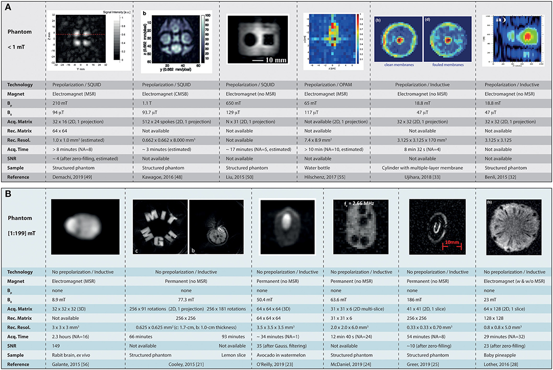
Figure 3. Summary of the current landscape of low-field MR imaging in phantoms. (A) Shows the major achievements obtained at ultra-low field (micro tesla range) in combination with SQUID detectors, and (B) the images obtained in the mT range (from 1 to 199 mT). MSR, magnetically shielded room; CMSB, compact magnetically shielded box; B_p, polarization field; NA, number of signal averaging. Images reused with permission from Cooley et al. [21], O'Reilly et al. [23], McDaniel et al. [24], Greer et al. [25], Lother et al. [28], Benli et al. [32], Ujihara et al. [33], Kawagoe et al. [48], Demachi et al. [49], Liu et al. [50], Hilschenz et al. [55]. Images reused from Galante et al. [56], held under Creative Commons License CC-BY 4.0.

MRI <1 mT

When considering ULF MRI with ultra-sensitive magnetometers, we can find more material from SQUID-based imaging as the latter technology is more mature. The work of Demachi et al. [49] shows pre-polarized 2D imaging (projection) at 4 kHz in a phantom composed of water and oil. From the parameters given it can be estimated that the minimum acquisition time was >8 min for a 2D 32 × 16 matrix interpolated to 64 × 64 in a phantom presenting four cylindrical columns (8-mm diameter, 19-mm depth), with a minimum polarization time of 0.125 s at B_p= 210 mT. The images displayed have extremely poor SNR. With a similar interest in food inspection application, Kawagoe et al. [48] show 2D imaging (projection) at ~94 μT (~4 kHz) in a 35-mm diameter, 8-mm thick phantom. A non-Cartesian radial acquisition scheme is used with 24 spokes, 512-ms acquisition time, and 5-s pre-polarization steps at B_p = 1.1 T (the highest reported here). The total acquisition time is not reported but could be estimated to ~3 min for an interpolated, reconstructed voxel size of 662 × 662 × 8, 000 μm³. Liu et al. [50] show the feasibility of imaging without an MSR in a 30 × 38 mm² (projection, no depth given) structured phantom at 129 μT (5.5 kHz). From the given image parameters, it can be estimated that the imaging time was ~17 min for their shortest phase encoding and acquisition times with a 5-s polarization at B_p= 650 mT. Cartesian acquisition was used in a spin-echo sequence with 31 phase-encode steps and number of average NA = 5 (no pixel size is given). The work of Hilschenz and colleagues shows 2D imaging (projection) with an OPAM operating at 117 μT (5 kHz) [55]. From a standard gradient echo approach following a 3-s pre-polarization step (B_p = 65 mT) and a total of NA = 10 averages, the team imaged the cross-section of a 34 mm-diameter bottle of di-ionized water. The given in-plane resolution of the 2D projection is 7.4 × 8.9 mm². SNR is not given, yet it looks quite poor. The total imaging time is not provided but can reasonably be expected to be above 10 min for a single projection from the parameters available. Benli [32] and Ujihara [33] have used inductive detection at 47 μT (~2 kHz) and a 2D spin-echo sequence (projections) in their commercial benchtop system. Ujihara and colleagues performed imaging in 8 min 32 s with echo times TE ranging from 200 to 800 ms, TR = 4000 ms, BW = 32 Hz, NA = 4, matrix size 32 × 32, FoV = 100 × 100 mm², for a reconstructed pixel size of 3.125 × 3.125 mm². The pre-polarization time was 2 s at 18.8 mT. Information on SNR is not being communicated. Benli and colleagues have shown 2D T₂-weighted images with similar matrix size, FoV, and BW, but with TE ranging from 140 to 400 ms, TR = 5 s, and 4.5 s pre-polarization steps. The number of averages and total acquisition times are not being communicated. The SNR appears rather poor but is not being communicated.

MRI From 1mT to 199 mT

Sitting at constant B₀= 8.9 mT static field (373 kHz), Galante and colleagues have shown MRI compatible with MEG settings in an MSR, but without pre-polarization [56]. Typical 3D Cartesian, spin-echo based acquisitions were performed with 32 × 32 × 32 matrix size, TE/TR = 19/500 ms, and a readout bandwidth in the kHz range. Scans in a doped water phantom and an ex vivo rabbit brain were acquired with 3 × 3 × 3 mm³ voxel size, NA = 1 in 8.5 min, and NA = 16 in 2.3 h, respectively. SNR of 70 is reported for NA = 1 in the phantom. SNR of 149 is reported for NA = 16 ex vivo. A 2D spin-echo based projection was also acquired with 32 × 32 matrix size and down to 1 × 1 × 1 mm³ voxel size in a ~3-cm diameter, ~10-mm high phantom filled with doped water. The latter shows rather poor SNR but no value is given. In their first attempt using a Halbach magnet geometry, Zimmerman-Cooley and colleagues were using the native field gradient from their magnet as a mean to perform spatial encoding [21]. The main advantage of such an approach is the simplicity of the design that does not require additional gradient or power electronics, thus facilitating flexibility and portability. The latter magnetic field gradients however are maximized in the periphery of the field of view with little or no gradient in the center, thus providing no spatial encoding (see Figure 3B). For their second iteration, the Boston team designed their magnet with an embedded linear gradient across the whole FoV, allowing spatial encoding from physically rotating the magnet around the object (multiple projections) [22], or by the addition of a gradient coil to modulate the latter in plane and sweep across k-space without rotation [58]. O'Reilly et al. [23] also report on imaging at 50.4 mT (2.15 MHz) using a custom Halbach magnet geometry. They acquired 3D images on a phantom composed of an avocado placed in a watermelon using a spin-echo sequence. Image parameters consisted in a 64 × 64 × 64 matrix with 220 × 220 × 220 mm³ FoV, resulting in a voxel size of ~3.5 × 3.5 × 3.5 mm³. The acquisition bandwidth was 20 kHz, with a TE/TR = 30/500 ms, and NA = 1. The resulting acquisition time was TA = ~34 min. Eventually, k−space data was filtered with a Gaussian filter before Fourier transform. The SNR in the images was reported to be ~35. In their compact MR cap geometry, McDaniel et al. [24] demonstrate 2D multi-slice imaging at 63.6 mT (2.67 MHz) in a 4-cm high, 6.3-cm wide structured phantom which size matches their targeted ROI. Six slices were acquired using a slice-interleaved RARE sequence. Acquisition matrix was 31 × 31 for a ~2 × 2 mm², 6-mm deep pixel resolution. The acquisition bandwidth was ~54 kHz, TR = 1,000 ms, echo spacing of 3 ms, and NA = 24 for a total acquisition time of 12 min 40 s. Greer et al. [25] in their portable device made of 5 permanent magnets also ventured into imaging at 186 mT (8 MHz). They could show 2D imaging (1 selected slice) from a spin-echo based sequence as described elsewhere [59]. Typical parameters were 41 × 41 2D acquisition matrices with centric ordering of k−space, interpolated to 256 × 256 for a default slice thickness of ~0.7 mm, and a pixel resolution of 0.33 × 0.33 mm². Reported SNR was ~10 with acquisition time TA = 54 min and NA = 8. Signal intensity changes from the highly inhomogeneous B₀ are corrected by dividing each image with a reference scan. The overall images do represent well the imaged objects, yet with severe geometric distortions. Relying on an electromagnet design, Lother et al. [28] have shown imaging at 23 mT (965 kHz) in their custom compact MRI system dedicated to neonates. 2D Spin-echo over a 5-mm thick slice is shown in a baby pineapple. The imaging parameters of the sequence used were TE/TR = 40/400 ms, FoV = 100 × 200 mm², matrix size 64 × 128, BW = 100 Hz, and averaging NA = 32 for a total acquisition time TA = 29 min. Interpolation from zero-filling in k−space allows to shrink the displayed pixels from ~1.6 × 1.6 mm² down to 0.8 × 0.8 mm². An SNR of 23 is reported on the displayed images.

In vivo Studies

Imaging in vivo applies to technology having reached a maturity level where most potential issues, hardware or software, are addressed to operate seamlessly in a living organism. The latter hence provides a better benchmark to assess performance such as SNR, contrast, and acquisition times in realistic objects and FoVs for future applications, being it clinical or pre-clinical. Figure 4 compiles all of the reported most recent low- and ultra-low field work in vivo.

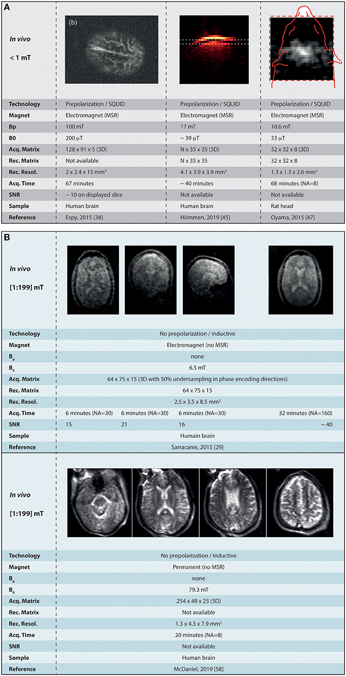
Figure 4. Summary of the current landscape of low-field MR imaging in vivo. (A) Shows the major achievements obtained at ultra-low field (micro tesla range) in combination with SQUID detectors, and (B) the images obtained in the mT range (from 1 to 199 mT). MSR, magnetically shielded room; CMSB, compact magnetically shielded box; B_p, polarization field; NA, number of signal averaging. Images reused, with permission, from Espy et al. [38], Hömmen et al. [45], Oyama et al. [47], McDaniel et al. [58]. Images reused from Sarracanie et al. [29], held under Creative Common License CC-BY 4.0.

MRI <1 mT

In the range under 1 mT (< 43 kHz), the most advanced work presenting in vivo imaging in humans was obtained using SQUIDs inside of an MSR [38]. In the latter, pre-polarized imaging in the human head was performed at 200 μT (8 kHz), with voxel size 2 × 2.4 × 15 mm³ using a 3D spin-echo sequence that includes 4 s pre-polarization steps at B_p= 100 mT, followed by a ~100-ms ramp before spatial encoding starts. The total imaging time was 67 min for the acquisition a 5-slice volume. The SNR on the 2nd slice is reported to be ~10, yet it drops drastically across the acquired volume. Similar in performance, Hömmen et al. [45] have performed pre-polarized imaging in vivo at lower field strength ~39 μT (1,645 Hz) in the human brain with 4.1 × 3.9 × 3.9 mm³ voxel size, from 35 k−steps in both 2^nd and 3^rd phase encoding directions. The sequence used was a 3D gradient-echo sequence with 500-ms pre-polarization steps at B_p= 17 mT, for a total acquisition time TA = 40 min. Only single slices are shown in 3 different orientations and SNRs are not reported. Finally, the work of Oyama shows imaging in a rat's head [47] at 33 μT (1.4 kHz) using 1 s pre-polarization steps at 10.6 mT peak field, and a 3D gradient echo acquisition with 32 × 32 × 8 matrix size. The total acquisition time was TA = 68 min for an 8-average scan (NA = 8) and voxel size 1.3 × 1.3 × 2.6 mm³. 2D images exhibit rather low SNR although values are not provided (cf Figure 4A).

MRI From 1 mT to 199 mT

Sitting at the very bottom of the range (6.5 mT or 276 kHz), Sarracanie and colleagues could show images in the living human brain [29] by making use of high efficiency balanced steady state free precession sequences. They report 3D 64 × 75 × 15 acquisition matrices with voxel resolution down to 2.5 × 3.5 × 8.5 mm³. Other parameters were TE/TR = 11/22.5 ms, number of averages NA = 30/160 and corresponding acquisition times TA = 6/32 min, using a 50% sampling rate with a variable density Gaussian pattern. The maximum SNR was reported to reach 15 (NA = 30) and ~40 (NA = 160) using the latter parameters. In the continuity of Zimmerman-Cooley's work in phantoms, McDaniel and colleagues reported on imaging in the living human head at 79 mT (~3.4 MHz) [58, 60]. Spin-echo sequences were employed using phase encoding for the 2^nd and 3^rd encoding spatial directions, along with frequency swept RF pulses so to provide coverage of nuclear spin frequencies over large magnetic field inhomogeneities [57]. They report 254 × 49 × 23 acquisition matrices providing 1.3 × 4.3 × 7.9 mm³ voxel size, with NA = 8, TE/TR = 148/3000 ms, and read-out bandwidth = 100 kHz, for a total acquisition time TA = 20 min. Efforts were made to passively shim the magnet from specific trays embedded in the original design, and a generalized reconstruction was performed and confronted to fast Fourier transform. The generalized reconstruction performs better than traditional Fourier, and although very encouraging, the reconstructed images exhibits some heavy distortions, in particular on the edges of the object where the magnetic field is most heterogeneous (see Figure 4B).

Sidetracks

The authors have tried to keep the extent of the present paper within a certain category of academic work and a specific time period, so to depict a refreshed view on the topic while keeping coherence for further discussion. Nonetheless, it is worth mentioning potent initiatives on the edge of our scope as some other contenders propose truly original approaches to MRI that also leverage low magnetic field strengths. At field strength ≥ 0.2 T, one start to enter the realm of low-field commercial systems less in line with the scope of the proposed overview. With a particular focus on mobility and accessibility, Nakagomi and colleagues have proposed a prototype, car-mounted MRI system operating at 0.2 T (8.5 MHz) [61]. Relying on a bi-planar permanent magnet architecture with a set of bi-planar gradient coils for spatial encoding, the team demonstrates 2D multi-slice imaging in the elbow within ~1 min 30 s. To the best of our knowledge, this is the first time that a full MRI system for human imaging is being sited in a standard, commercial vehicle. This initiative, even at the stage of prototyping, advocates strongly for the use of lower field technology to promote flexibility in future mobile systems. Similarly, low static magnetic field (0.35 T or 14.9 MHz) was successfully employed in the first CE marked (and FDA cleared) MRI-guided radiation therapy cancer treatment system by ViewRay (MRIdian Linac, ViewRay Inc., Oakwood, USA) [62]. It further demonstrates that bringing down magnetic field is a relevant option to combine complex and rather incompatible modalities within the same device. Balanced steady state (b-SSFP) based MRI sequences are used that are particularly well-suited to low-field. From an increased $\frac{T_2}{T_1}$ ratio, the transverse magnetization at steady-state is increased that promotes SNR [63], and from lower sensitivity to magnetic field inhomogeneity, the images acquired are less prone to typical banding artifact encountered at higher field [29]. Another growing interest in MRI lies in the acquisition of quantified metrics to replace the long-lasting legacy of reading shades of gray. Field cycling relaxometry is a technique that started to be used in NMR spectroscopy, which consists in measuring the longitudinal relaxation rate T₁ in samples at multiple field strengths [64–67]. T₂ relaxation would probably need some deeper investigation in the low-field range, but is currently less of interest due to little dependence with field strength [68]. T₁ on the contrary is known to exhibit clear changes. Its evolution as a function of field is not linear and hence can be used as an extra degree of freedom to characterize tissue types, and potentially help in the identification of new biomarkers for a given pathology. At low field in particular, the dispersion in T₁ relaxation rates is much bigger than at clinical field strength (or higher) and moves away from that of pure water as more and more molecular motion contribute to relaxation processes [69]. Since it is commonly accepted that the water content of tissue is neither tissue nor disease dependent, the MR community probably should embrace the exploration of new paths for diagnosis purpose. Regarding its application in MRI however, relaxometry is not used in clinical routine due to the additional time needed to probe the NMR signal at multiple time points. Accounting for the multiple time points necessary, the multiple static magnetic field strength to be investigated, and the loss of SNR intrinsic to lower proton magnetization, it might be hard to imagine field cycling approaches being implemented with future clinical low field MRI systems. Despite these challenges, a group of researchers from the University of Aberdeen has however managed to build the first whole body Fast Field-Cycling MRI scanner and used it for clinical molecular imaging studies [70]. With all legal authorizations to conduct studies in human volunteers and patients, the team has managed to provide T₁ dispersion maps in vivo in the living human breast, brain and knee that already points toward contrasts and diagnostic capability unique to low field. The total duration of FFC-MRI scans varied between 35 and 50 min from positioning of the patient to withdrawal. With a constant detection field of 0.2 T (8.5 MHz) higher than reported in this paper, the range of investigated T₁s spans nonetheless from 50 μT to 0.2 T, hence very low field strengths.

Commercial Perspectives

If the research at very low-field strength seems to be quite dynamic again, it is still hard to predict what will eventually result in commercial solutions for clinical practice in the long term. In order to add value and potentially find new markets, it is reasonable to assume that such devices will not be designed to compete with high-field settings, but instead address current needs where they can be complementary and accessible. Amongst the main avenues considered, systems to be sited in emergency units, in the operating room or even in the field will likely be developed for applications in neurology or musculoskeletal disorders, where some well-defined needs already exist (e.g. stroke diagnosis). With a permanent, bi-planar magnet architecture operating at 64 mT (~2.7 MHz), the first and only contender to a commercial, accessible and mobile MRI comes from Hyperfine (Guilford, CT, USA), an American start-up company that just unveiled their MRI system in late 2019. The whole MRI system and embedded electronics is mounted on a cart with motorized wheels and can be plugged into a standard wall outlet. It has not yet been cleared with CE approval, but was recently granted 510(k) FDA clearance and is currently being tested in several clinical settings on the east-coast of the United States. With no specific need for siting and low power requirement, it can easily be placed in the emergency department, the neuro-intensive care or pediatric units. It was first intended for neuro-imaging and muskulo-skeletal applications. At a different scale, it is worth mentioning that the main manufacturers also seem to be reconsidering their position toward low-field MRI. In their first attempt, low-field was only considered for open access permanent magnet based devices, which reduced cost did not allow to increase the overall value, mainly due to important siting requirements and disadvantaged by overall inferior performance. To the best of our knowledge, no commercial device is foreseen yet, but a recent publication has communicated about one of the main manufacturers (Siemens Healthineers, Erlangen, Germany) ramping a clinical 1.5 T (~64 MHz) scanner down to 0.55 T (23.4 MHz) for a variety of applications [15]. Benefiting from lower sensitivity to magnetic susceptibility effects and enhanced contrast in the mid-field regime, it has resulted in a series of preliminary results recently communicated by the same group [71–74].

Discussion

In this paper, a rather extensive review of the current landscape of low to ultra-low field MRI has been listed and described. We decided to focus on the last 5 years of development to give a fresh view on the topic, though we encourage the reader to learn more about older inspiring pioneer work in the field. Indeed, very interesting research has been published especially in the late 80s—early 90s [1, 4, 75–77], with a brief recurring interest in the early 2000s, in particular for interventional applications [13, 14]. The MR community is clearly entering one of those cycles where the interest in low- and ultra-low field MRI is raising again, and the past few years have shown a remarkable increase of communications regarding new hardware and imaging techniques. In this context, we try to present an exhaustive list of approaches reflecting the current research effort, all of which is capable of generating images at field strengths as low as a few μT. From this “snapshot” of the current state of the art, it is possible to take some perspective and discuss what seems to be most relevant, at least in the short and medium term, or what kind of technological locks would need to be addressed in order for some approaches to work. Indeed, not all of the work presented has a potential to translate into in vivo and further into clinical applications, the main reason being that such settings require simple-to-use, rugged and rather fast technologies. The authors anticipate that pre-polarizing approaches that are quite well-represented in low field research might have difficulties to meet clinical needs both on the infrastructure and performance levels. It is indeed quite striking to observe that when using pre-polarization, often more than 95% of the examination time is being used field cycling and not acquiring data. We can notice that while sensitivity is already quite reduced from working at weaker field strength, the low duty cycle on the acquisition side is never quite compensated by a higher (even very high [48]) pre-polarizing field or higher sensitivity sensors. One might consider using that time to acquire and average data as a more efficient way to increase SNR, with the added benefit of simpler setups if field cycling is not required. In addition, the longer readout and encoding times generally encountered added with incompressible delays to cycle down the pre-polarization fields also penalize signals with short lifetimes, and one may end up only being able to probe species with long relaxation time such as free water compartments as seen with Espy and colleagues [38] (Figure 4A). Pre-polarization techniques are often employed for magneto-encephalography in conjunction with high sensitivity magnetometers but new insights for alternatives are proposed, such as in the work from Galante [31, 56]. Imaging at thermal equilibrium without pre-polarization seems to be the most promising approach considering the image quality achievable today. Permanent and resistive magnets are two good candidates that have both pros and cons. Permanent magnet architectures have the big advantage of requiring no power, key to the prospect of future small footprint, accessible technology. The achievable field homogeneity however is easily one to two orders of magnitude worse than what can be found in resistive magnets. As a result, strong artifacts that impede image quality can be seen in all of the studies presented (Figures 3, 4), that are very hard to correct. Innovative reconstruction methods will be required to overcome this difficulty, probably moving away from typical Fourier frameworks, and leveraging for example deep learning approaches. If this technical challenge has not yet been unlocked, addressing this reconstruction issue has the potential to truly disrupt the field. Permanent magnets also suffer from poor field stability with respect to temperature, which certainly interrogates on their deployment in extreme environments without controlled temperature and humidity. On the other hand, resistive magnet architectures provide better field homogeneity and the ability to change the desired field of operation or even switch it off, but at the cost of higher power needs as well as cooling. Then, depending on the targeted magnet size and field strength, simple cooling solutions are foreseeable (forced air vs. water) before requiring any complex or demanding cooling resources. Eventually, both permanent and resistive magnet technologies are worth exploring when it comes to low and ultra-low field imaging, keeping in mind the requirements and constraints for the targeted applications and corresponding working environments. A general comment in view of the multiple attempts to build smaller magnets could be to assess imaging capability first in a controlled setting before construction is envisioned. That could be an efficient way to save time on such developments, rather than empirically iterating on complex magnet construction and later realize whether or not imaging is feasible. Regarding field strength, it is quite interesting to note that all the attempts to low-field imaging reported here cover quite a broad range, and that a higher field strength does not bring superior image quality (Figures 3, 4). Overall, the range 5–100 mT appears to be the most promising in delivering fast imaging in vivo, at both extremities of the spectrum [24, 29]. From the latter results, we believe that the democratization of low field MRI will not come from reaching higher fields, but instead being able to stay low. The key is to embrace the advantages offered by this unique regime while gathering a set of technological solutions that maximize SNR/unit time (i.e., from sensors, acquisition schemes) and navigate through magnetic field inhomogeneity. Further, we believe that approaches such as model-based MRI and deep learning will appear of upmost relevance to navigate through poor SNR, while promoting access to simpler hardware and hence lower cost and reduced physical footprint. Another major and often overlooked feature of low-field MRI deserves further discussion: contrast. It is known from the early days of MRI that low-field strengths provide a higher dispersion in T₁ relaxation times [78] (see Figure 5) but the latter never really was extensively explored. Many scientists may be working with “standard” high-field commercial equipment and completely be missing which field strength provides the best contrast (i.e., T₁, T₂ dispersion) with respect to their individual interests. An interesting change of paradigm could be envisioned where exploratory studies would be performed in dedicated MR systems, ramping the field in order to assess the dispersion in relaxation rates and potentially finding the sweet spot for maximum contrast. Eventually, future generations of low-field MRI systems with field cycling possibilities could be anticipated where contrast can be tuned to a specific application. The latter is not too far away from current fast-field cycling MRI initiatives described above in this manuscript, aimed at uncovering T₁ dispersion as an intrinsic metric of interest in MRI diagnosis [70]. Naturally, such considerations on contrast open new perspectives regarding diagnosis capability, yet it will also challenge radiologists to adapt their skills in the interpretation of images according to the field strength of operation. It may also be in the hands of other practitioners to complement radiologists and develop basic skills at reading images (as many already do), such that new class of point-of-care units truly succeed to decongest radiology departments. Alternatively, one may see these devices more as tools to answer simple clinical questions, rather than a complex imaging device that belong to the radiology department. Coming back to the title of this paper and its question how low can we go? our experience suggests that it is likely to be an ill-posed problem. The question should be application-driven and address specific goals as well as technical constraints. Let us go back in time and make an analogy with aerospace research. The question in the 1960s was: “what technological leap is needed to go on the moon?” and not “what technology should we build in order to explore the entire galaxy?” In medical imaging, scientists and clinicians have adapted ultrasound or X-ray-based modalities to address challenges in different disciplines of medicine. MRI on the other hand has been almost untouched for the last three decades and one-fits-all scanners continue to be the main stream. As a consequence, MRI has become a bottleneck in the hospital care chain for 50% of the total world population, and the pecuniary burden linked to scanner purchase, siting and maintenance makes it inaccessible for the remaining 50% (see Figure 6). Indeed, cost is undeniably an issue in the accessibility of MRI technology. If financial support can always be found for a one-time purchase, it is difficult to find resources for costly maintenance contracts or simply to maintain infrastructure over long time periods, as infrastructure can also be of critical importance. Examples include recurring power outages, either because of lack of financial means in developing countries, or in war zones. Electricity blackouts can severely damage medical devices that will never be repaired and pile-up in endless medical device graveyards. Leveraging low magnetic field in scanners addressing these difficulties would certainly open a market in such regions, very similar to what the start-up company Pristem SA did with their robust and low-cost X-ray system GlobalDiagnostiX (Pristem SA, Lausanne, Switzerland). Accessibility is also bound to siting resources. Standard MRI units require three separate rooms: one for the operator, the RF and magnetically shielded examination room, and the technical room with all the associated power electronics. Highly populated regions, like most major cities in Asia, often have the means to buy MRI machines, but not to site them. Low field alternatives that do not need specific shielding or heavy power requirements certainly would address this challenge and again open an untouched market. For the wealthiest half of the world population, low-field MRI dedicated to a range or a specific application (neurology, MSK, etc.), has the potential to decongest radiology departments and also facilitate magnetic resonance in multi-modal settings from an intrinsic enhanced compatibility. Sited outside of the radiology department, such MRI units would become handy tools to the practitioner, accessible to all disciplines and population, and hence start to change paradigm from the historical one-fits-all. The same approach might ultimately follow at high and ultra-high field where the application envisioned will lead manufacturers to offer purpose-built systems that fit the needs of research and medical professionals. Unless one wants to address the underlying question: how high shall we go for high-field MRI?

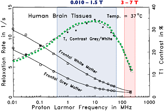
Figure 5. Relative T₁ contrast in human brain samples as a function of Larmor frequency. The green dotted line shows that the relative contrast between gray and white matter is higher when operating between 10 mT and 1.5 T (shaded blue box) and decreases dramatically at very high to ultra-high field strengths (shaded red box). Modified, with permission, from Fischer et al. [78].

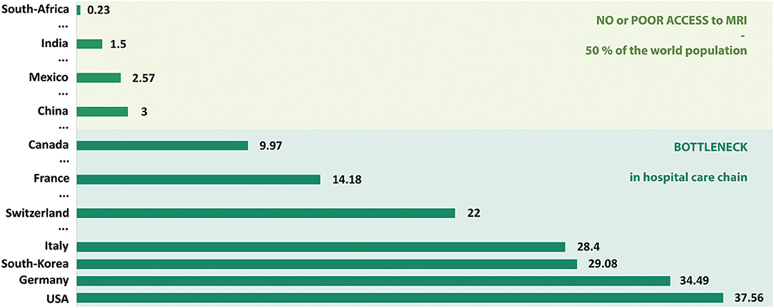
Figure 6. Number of MRI units per million population. Only a sample of countries are presented here in order to simply illustrate the current MRI market worldwide. Data extracted mainly from Statistica.com, 2017 reports.

Conclusion

Low field MRI has regained popularity over the past few years, reopening the debate on its relevance in the clinical setting. With half of the world population underserved regarding MR diagnosis, the medical community indeed strives for more ubiquitous and accessible systems. Lowering magnetic field strength opens new perspectives to increase MR value not only from reduced costs, but also from enhanced outcomes, shifting paradigm toward specific use cases and more adaptability. It promotes new magnet geometries that have already performed imaging in vivo in humans, and which low-footprint core technology is no longer associated with superconductive materials. Lower field MRI as such could diversify the current offer to a broader range of medical applications and geographical locations, with a wider range of contrasts to complement current diagnostic tools. As a conclusion, we believe that it is time to go as low as diagnostically relevant. It is the scientific and medical communities' responsibility to choose how low/high one should go depending on specific applications, and to work side-by-side with the industry to build the future of MRI diagnosis.

Author Contributions

All authors listed have made a substantial, direct and intellectual contribution to the work, and approved it for publication.

Funding

This work was supported by the Swiss National Science Foundation (grants #PP00P2_170575; PCEFP2_186861).

Conflict of Interest

MS is a co-founder and former member of Hyperfine Research Inc.

The remaining author declares that the research was conducted in the absence of any commercial or financial relationships that could be construed as a potential conflict of interest.

References

1. Sepponen RE, Sipponen JT, Sivula A. Low-field (20mT) NMRI of the brain. J Comput Assist Tomogr. (1985) 9:237–41. doi: 10.1097/00004728-198503000-00002
2. Sipponen JT, Sepponen RE, Tanttu JI, Sivula A. Intracranial hematomas studied by MRI at 0.17 and 0.02 T. J Comput Assist Tomogr. (1985) 9:698–704. doi: 10.1097/00004728-198507010-00007
3. Hovi I, Korhola O, Valtonen M, Valtonen V, Taavitsainen M, Kivisaari A, et al. Detection of soft-tissue and skeletal infections with ultra low-field (0.02 T) MRI. Acta Radiol. (1989) 30:495–9. doi: 10.3109/02841858909175316
4. Constantinesco A, Arbogast S, Foucher G, Vinée P, Choquet P. Detection of glomus tumor of the finger by dedicated MRI at 0.1 T. Magn Reson Imaging. (1984) 12:1131–4. doi: 10.1016/0730-725X(94)91246-S
5. Kaufman L. The Impact Of Radiology's Culture On The Cost Of Magnetic Resonance Imaging. J Magn Reson Imaging. (1996) 68:67–71. doi: 10.1002/jmri.1880060113
6. Edelman RR. The History of MR imaging as seen through the pages of radiology. Radiology. (2014) 273:S181–200. doi: 10.1148/radiol.14140706
7. Moser E, Laistler E, Schmitt F, Kontaxis G. Ultra-high field NMR and MRI—the role of magnet technology to increase sensitivity and specificity. Front Phys. (2017) 5:33. doi: 10.1016/S0140-6736(11)60282-1
8. Zimmerman RA, Bilaniuk LT, Hackney DB, Goldberg HI, Grossman RI. Head injury: early results of comparing CT and high-field MR. AJR. (1986) 147:1215–22. doi: 10.2214/ajr.147.6.1215
9. Choquet P, Breton E, Goetz C, Marin C, Constantinesco A. Dedicated low-field MRI in mice. Phys Med Biol. (2009) 54:5287–99. doi: 10.1111/j.1740-8261.1995.tb00306.x
11. van Beek EJR, Kuhl C, Anzai Y, Desmond P, Ehman RL, Gong Q, et al. Value of MRI in medicine: more than just another test? J Magn Reson Imaging. (2019) 49:e14–25. doi: 10.1148/radiol.2016150789
12. Iturri-Clavero F, Galbarriatu-Gutierrez L, Gonzalez-Uriarte A, Tamayo-Medel G, de Orte K, Martinez-Ruiz A, et al. “Low-field” intraoperative MRI: a new scenario, a new adaptation. Clin Radiol. (2016) 71:1193–8. doi: 10.1016/j.crad.2016.07.003
13. Senft C, Ulrich CT, Seifert V, Gasser T. Intraoperative magnetic resonance imaging in the surgical treatment of cerebral metastases. J Surg Oncol. (2010) 10:436–41. doi: 10.1007/s11060-009-9868-6
14. Senft C, Seifert V, Hermann E, Gasser T. Surgical treatment of cerebral abscess with the use of a mobile ultralow-field MRI. Neurosurg Rev. (2008) 32:77–85. doi: 10.1016/0090-3019(93)90008-O
15. Campbell-Washburn AE, Ramasawmy R, Restivo MC, Bhattacharya I, Basar B, Herzka DA, et al. Opportunities in interventional and diagnostic imaging by using high-performance low-field-strength MRI. Radiology. (2019) 293:384–93. doi: 10.1148/radiol.2019190452
16. Schukro C, Puchner SB. Safety and efficiency of low-field magnetic resonance imaging in patients with cardiac rhythm management devices. Eur J Radiol. (2019) 118:96–100. doi: 10.1016/j.ejrad.2019.07.005
17. Klein HM. Clinical Low Field Strength Magnetic Resonance Imaging. Cham: Springer International Publishing AG Switzerland (2016). doi: 10.1007/978-3-319-16516-5
18. Hoult DI, Richards RE. The signal-to-noise ratio of the nuclear magnetic resonance experiment. J Magn Reson. (1976) 24:71–85. doi: 10.1016/j.jmr.2011.09.018
19. Marques JP, Simonis FFJ, Webb AG. Low-field MRI: an MR physics perspective. J Magn Reson Imaging. (2018) 49:1528–42. doi: 10.1002/mrm.26221
20. Darrasse L, Ginefri JC. Perspectives with cryogenic RF probes in biomedical MRI. Biochimie. (2003) 85:915–37. doi: 10.1016/j.biochi.2003.09.016
21. Cooley CZ, Stockmann JP, Armstrong BD, Sarracanie M, Lev MH, Rosen MS, et al. Two-dimensional imaging in a lightweight portable MRI scanner without gradient coils. Magn Reson Med. (2015) 73:872–83. doi: 10.1002/mrm.25147
22. Cooley CZ, Haskell MW, Cauley SF, Sappo C, LaPierre CD, Ha CG, et al. Design of sparse Halbach magnet arrays for portable MRI using a genetic algorithm. IEEE Trans Magn. (2018) 54:1–12. doi: 10.1109/TMAG.2017.2751001
23. O'Reilly T, Teeuwisse WM, Webb AG. Three-dimensional MRI in a homogenous 27 cm diameter bore Halbach array magnet. J Magn Reson. (2019) 307:106578. doi: 10.1016/j.jmr.2019.106578
24. McDaniel PC, Cooley CZ, Stockmann JP, Wald LL. The MR Cap: a single-sided MRI system designed for potential point-of-care limited field-of-view brain imaging. Magn Reson Med. (2019) 82:1946–60. doi: 10.1006/jmre.2000.2263
25. Greer M, Chen C, Mandal S. An easily reproducible, hand-held, single-sided, MRI sensor. J Magn Reson. (2019) 308:106591. doi: 10.1016/j.jmr.2019.106591
26. Eidmann G, Savelsberg R, Peter B, Blümich B. The NMR MOUSE, a mobile universal surface explorer. J Magn Reson. (1996) 122:104–9. doi: 10.1006/jmra.1996.0185
27. Blümich B, Peter B, Guthausen A, Haken R, Schmitz U, Saito K, et al. The NMR-MOUSE: construction, excitation, and applications. Magn Reson Imaging. (1998) 16:479–84. doi: 10.1016/S0730-725X(98)00069-1
28. Lother S, Schiff SJ, Neuberger T, Jakob PM, Fidler F. Design of a mobile, homogeneous, and efficient electromagnet with a large field of view for neonatal low-field MRI. Magn Reson Mater Phys. (2016) 29:691–8. doi: 10.1007/s10334-016-0525-8
29. Sarracanie M, LaPierre CD, Salameh N, Waddington DEJ, Witzel T, Rosen MS. Low-cost high-performance MRI. Sci Rep. (2015) 5:15177. doi: 10.1038/srep15177
30. Tsai LL, Mair RW, Rosen MS, Patz S, Walsworth RL. An open-access, very-low-field MRI system for posture-dependent 3He human lung imaging. J Magn Reson. (2008) 193:274–85. doi: 10.1016/j.jmr.2008.05.016
31. Galante A, Catallo N, Sebastiani P, Sotgiu A, Sinibaldi R, De Luca C, et al. Very Low Field MRI: a Fast System Compatible with Magnetoencephalography. Turin: IEEE MeMeA Proc. (2015) 560–4. doi: 10.1109/MeMeA.2015.7145266
32. Benli KP, Dillmann B, Louelh R, Poirier-Quinot M, Darrasse L. Illustrating the quantum approach with an Earth magnetic field MRI. Eur J Phys. (2015) 36:035032. doi: 10.1038/334019c0
33. Ujihara R, Fridjonsson EO, Bristow NW, Vogt SJ, Bucs SS, Vrouwenvelder JS, et al. Earth's field MRI for the non-invasive detection of fouling in spiral-wound membrane modules in pressure vessels during operation. Desalin Water Treat. (2018) 135:16–24. doi: 10.5004/dwt.2018.23156
34. Zotev VS, Matlashov AN, Volegov PL, Savukov IM, Espy MA, Mosher JC, et al. Microtesla MRI of the human brain combined with MEG. J Magn Reson. (2008) 194:115–20. doi: 10.1016/j.jmr.2008.06.007
35. Zotev VS, Volegov PL, Matlashov AN, Espy MA, Mosher JC, Kraus RH Jr. Parallel MRI at microtesla fields. J Magn Reson. (2008) 192:197–208. doi: 10.1016/j.jmr.2008.02.015
36. Volegov P, Flynn M, Kraus R, Magnelind P, Matlashov A, Nath P, et al. Magnetic resonance relaxometry at low and ultra low fields. IFMBE Proc. (2010) 28:82–7. doi: 10.1007/978-3-642-12197-5_15
37. Vesanen PT, Zevenhoven KCJ, Nieminen JO, Dabek J, Parkkonen LT, Ilmoniemi RJ. Temperature dependence of relaxation times and temperature mapping in ultra-low-field MRI. J Magn Reson. (2013) 235:50–7. doi: 10.1016/j.jmr.2013.07.009
38. Espy MA, Magnelind PE, Matlashov AN, Newman SG, Sandin HJ, Schultz LJ, et al. Progress toward a deployable SQUID-based ultra-low field MRI system for anatomical imaging. IEEE Trans Appl Supercond. (2015) 25:1–5. doi: 10.1109/TASC.2014.2365473
39. McDermott R, Lee S, Haken te B, Trabesinger AH, Pines A, Clarke J. Microtesla MRI with a superconducting quantum interference device. Proc Natl Acad Sci USA. (2004) 101:7857–61. doi: 10.1073/pnas.0402382101
40. Inglis B, Buckenmaier K, SanGiorgio P, Pedersen AF, Nichols MA, Clarke J. MRI of the human brain at 130 microtesla. Proc Natl Acad Sci USA. (2013) 110:19194–201. doi: 10.1073/pnas.1319334110
41. Ganssle PJ, Shin HD, Seltzer SJ, Bajaj VS, Ledbetter MP, Budker D, et al. Ultra-Low-Field NMR relaxation and diffusion measurements using an optical magnetometer. Angew Chem. (2014) 126:9924–8. doi: 10.1063/1.3623024
42. Lin FH, Vesanen PT, Hsu YC, Nieminen JO, Zevenhoven KCJ, Dabek J, et al. Suppressing multi-channel ultra-low-field MRI measurement noise using data consistency and image sparsity. PLoS ONE. (2013) 8:e61652. doi: 10.1371/journal.pone.0061652.g005
43. Clarke J, Hatridge M, Mößle M. SQUID-detected magnetic resonance imaging in microtesla fields. Annu Rev Biomed Eng. (2007) 9:389–413. doi: 10.1146/annurev.bioeng.9.060906.152010
44. Dong H, Zhang Y, Krause HJ, Xie X, Offenhäusser A. Low field MRI detection with tuned HTS SQUID magnetometer. IEEE Trans Appl Supercond. (2011) 21:509–13. doi: 10.1109/TASC.2010.2091713
45. Hömmen P, Storm JH, Höfner N, Körber R. Demonstration of full tensor current density imaging using ultra-low field MRI. Magn Reson Imaging. (2019) 60:137–44. doi: 10.1016/j.mri.2019.03.010
46. Drung D, Assmann C, Beyer J, Kirste A, Peters M, Ruede F, et al. Highly sensitive and easy-to-use SQUID sensors. IEEE Trans Appl Supercond. (2007) 17:699–704. doi: 10.1109/TASC.2007.897403
47. Oyama D, Higuchi M, Kawai J, Tsuyuguchi N, Miyamoto M, Adachi Y, et al. Measurement of Magnetic Resonance Signal from a Rat Head in Ultra-low Magnetic Field. Nagoya: ISEC Proc. (2015) 1–3. doi: 10.1109/ISEC.2015.7383470
48. Kawagoe S, Toyota H, Hatta J, Ariyoshi S, Tanaka S. Ultra-low field MRI food inspection system prototype. Phys C. (2016) 530:104–8. doi: 10.1016/j.physc.2016.02.015
49. Demachi K, Hayashi K, Adachi S, Tanabe K, Tanaka S. T1-weighted image by ultra-low field SQUID-MRI. IEEE Trans Appl Supercond. (2019) 29:1600905. doi: 10.1109/TASC.2019.2902772
50. Liu C, Chang B, Qiu L, Dong H, Qiu Y, Zhang Y, et al. Effect of magnetic field fluctuation on ultra-low field MRI measurements in the unshielded laboratory environment. J Magn Reson. (2015) 257:8–14. doi: 10.1016/j.jmr.2015.04.014
51. Savukov I, Karaulanov T, Castro A, Volegov P, Matlashov A, Urbatis A, et al. Non-cryogenic anatomical imaging in ultra-low field regime: Hand MRI demonstration. J Magn Reson. (2011) 211:101–8. doi: 10.1016/j.jmr.2011.05.011
52. Savukov I, Karaulanov T. Anatomical MRI with an atomic magnetometer. J Magn Reson. (2013) 231:39–45. doi: 10.1016/j.jmr.2013.02.020
53. Savukov I, Karaulanov T, Wurden CJV, Schultz L. Non-cryogenic ultra-low field MRI of wrist–forearm area. J Magn Reson. (2013) 233:103–6. doi: 10.1016/j.jmr.2013.05.012
54. Savukov I, Karaulanov T. Magnetic-resonance imaging of the human brain with an atomic magnetometer. Appl Phys Lett. (2013) 103:043703. doi: 10.1109/TASC.2009.2018764
55. Hilschenz I, Ito Y, Natsukawa H, Oida T, Yamamoto T, Kobayashi T. Remote detected low-field MRI using an optically pumped atomic magnetometer combined with a liquid cooled pre-polarization coil. J Magn Reson. (2017) 274:89–94. doi: 10.1016/j.jmr.2016.11.006
56. Galante A, Sinibaldi R, Conti A, De Luca C, Catallo N, Sebastiani P, et al. Fast room temperature very low field-magnetic resonance imaging system compatible with MagnetoEncephaloGraphy environment. PLoS ONE. (2015) 10:e0142701. doi: 10.1371/journal.pone.0142701.g011
57. Stockmann JP, Cooley CZ, Guerin B, Rosen MS, Wald LL. Transmit array spatial encoding (TRASE) using broadband WURST pulses for RF spatial encoding in inhomogeneous B0 fields. J Magn Reson. (2016) 268:36–48. doi: 10.1016/j.jmr.2016.04.005
58. McDaniel PC, Cooley CZ, Stockmann JP, Wald LL. A target-field shimming approach for improving the encoding performance of a lightweight Halbach magnet for portable brain MRI. In: Proceedings of the International Society for Magnetic Resonance in Medicine. Montreal (2019). p. 0215.
59. Perlo J, Casanova F, Blümich B. 3D imaging with single-sided sensor: an open tomograph. J Magn Reson. (2004) 166:228–35. doi: 10.1016/j.jmr.2003.10.018
60. McDaniel PC, Cooley CZ, Stockmann JP, Wald LL. 3D imaging with a portable MRI scanner using an optimized rotating magnet and 1D gradient coil. In: Proceedings of the International Society for Magnetic Resonance in Medicine. Paris (2018). p. 0029.
61. Nakagomi M, Kajiwara M, Matsuzaki J, Tanabe K, Hoshiai S, Okamoto Y, et al. Development of a small car-mounted magnetic resonance imaging system for human elbows using a 0.2 T permanent magnet. J Magn Reson. (2019) 304:1–6. doi: 10.1016/j.jmr.2019.04.017
62. Klüter S. Technical design and concept of a 0.35 T MR-Linac. Clin Transl Radiat Oncol. (2019) 18:98–101. doi: 10.1016/j.ctro.2019.04.007
63. Scheffler K, Lehnhardt S. Principles and applications of balanced SSFP techniques. Eur Radiol. (2003) 13:2409–18. doi: 10.1007/s00330-003-1957-x
64. Koenig SH, Hallenga K, Shporer M. Protein-water interaction studied by solvent 1H, 2H, and 17O magnetic relaxation. Proc Natl Acad Sci USA. (1975) 72:2667–71. doi: 10.1073/pnas.72.7.2667
65. Grösch L, Noack F. NMR relaxation investigation of water mobility in aqueous bovine serum albumin solutions. Biochim Biophys Acta BBA. (1976) 453:218–32. doi: 10.1016/0005-2795(76)90267-1
66. Kimmich R. Field cycling in NMR relaxation spectroscopy: applications in biological, chemicaland polymer physics. Bull Magn Reson. (1980) 1:195–218.
67. Noack F. NMR field-cycling spectroscopy: principles and applications. Prog Nucl Magn Reson Spectrosc. (1986) 18:171–276. doi: 10.1016/0079-6565(86)80004-8
68. Bottomley PA, Foster TH, Argersinger RE, Pfeifer LM. A review of normal tissue hydrogen NMR relaxation times and relaxation mechanisms from 1-100 MHz: dependence on tissue type, NMR frequency, temperature, species, excision, and age. Med Phys. (1998) 11:425–48. doi: 10.1118/1.595535
69. Rinck PA, Fischer HW, Vander Elst L, Van Haverbeke Y, Muller RN. Field-cycling relaxometry: medical applications. Radiology. (1988) 168:843–9. doi: 10.1148/radiology.168.3.3406414
70. Broche LM, Ross PJ, Davies GR, MacLeod MJ, Lurie DJ. A whole-body Fast Field-Cycling scanner for clinical molecular imaging studies. Sci Rep. (2019) 9:10402. doi: 10.1038/s41598-019-46648-0
71. Basar B, Sonmez M, Paul R, Kocaturk O, Herzka DA, Lederman RJ, et al. Ferromagnetic markers for interventional MRI devices at 0.55 T. In: Proceedings of the International Society for Magnetic Resonance in Medicine. Montreal (2019) p. 3845.
72. Bhattacharya I, Ramasawmy R, McGuirt DR, Mancini C, Lederman RJ, Moss J, et al. Improved lung imaging and oxygen enhancement at 0.55 T. In: Proceedings of the International Society for Magnetic Resonance in Medicine. Montreal (2019) p. 0003.
73. Restivo MC, Ramasawmy R, Herzka DA, Campbell-Washburn AE. Long TR bSSFP cardiac cine imaging at low field (0.55 T) using EPI and spiral sequences for improved sampling efficiency. In: Proceedings of the International Society for Magnetic Resonance in Medicine. Montreal (2019) p. 1084.
74. Ramasawmy R, Herzka DA, Restivo MC, Bhattacharya I, Lederman RJ, Campbell-Washburn AE. Spin-echo imaging at 0.55 T using a spiral trajectory. In: Proceedings of the International Society for Magnetic Resonance in Medicine. Montreal (2019). p. 1192.
75. Gries P, Constantinesco A, Brunot B, Facello A. MRI of hand and wrist with a dedicated 0.1-T low-field imaging system. Magn Reson Imaging. (1991) 9:949–53. doi: 10.1016/0730-725X(91)90541-S
76. Lotz H, Ekelund L, Hietala SO, Wickman G. Low field (0.02 T) MRI of the whole body. J Comput Assist Tomogr. (1988) 12:1006–13. doi: 10.1097/00004728-198811000-00018
77. Claudon M, Darrasse L, Boyer B, Regent D, Sauzade M. L'IRM à champ modéré. Rev Im Med. (1991) 3:151–8.
Keywords: MRI, low magnetic field, ultra-low field MRI, MR value, point-of-care MRI
Citation: Sarracanie M and Salameh N (2020) Low-Field MRI: How Low Can We Go? A Fresh View on an Old Debate. Front. Phys. 8:172. doi: 10.3389/fphy.2020.00172
Received: 04 February 2020; Accepted: 23 April 2020;
Published: 12 June 2020.
Edited by:
Ewald Moser, Medical University of Vienna, AustriaReviewed by:
Angelo Galante, University of L'Aquila, ItalyMarie Poirier-Quinot, Université Paris-Sud, France
Copyright © 2020 Sarracanie and Salameh. This is an open-access article distributed under the terms of the Creative Commons Attribution License (CC BY). The use, distribution or reproduction in other forums is permitted, provided the original author(s) and the copyright owner(s) are credited and that the original publication in this journal is cited, in accordance with accepted academic practice. No use, distribution or reproduction is permitted which does not comply with these terms.
*Correspondence: Mathieu Sarracanie, mathieu.sarracanie@unibas.ch