 Yeong-Hun Song1
 Jun-Young Yi1Young Noh2
 Hyemin Jang3Sang Won Seo3Duk L. Na3Joon-Kyung Seong1,4,5*
  for the Alzheimer’s Disease Neuroimaging Initiative†
- 1Department of Artificial Intelligence, Korea University, Seoul, South Korea
- 2Department of Neurology, Gil Medical Center, Gachon University College of Medicine, Incheon, South Korea
- 3Department of Neurology, Samsung Medical Center, School of Medicine, Sungkyunkwan University, Seoul, South Korea
- 4School of Biomedical Engineering, Korea University, Seoul, South Korea
- 5Interdisciplinary Program in Precision Public Health, College of Health Science, Korea University, Seoul, South Korea
Structural changes in the brain due to Alzheimer’s disease dementia (ADD) can be observed through brain T1-weighted magnetic resonance imaging (MRI) images. Many ADD diagnostic studies using brain MRI images have been conducted with machine-learning and deep-learning models. Although reliability is a key in clinical application and applicability of low-resolution MRI (LRMRI) is a key to broad clinical application, both are not sufficiently studied in the deep-learning area. In this study, we developed a 2-dimensional convolutional neural network-based classification model by adopting several methods, such as using instance normalization layer, Mixup, and sharpness aware minimization. To train the model, MRI images from 2,765 cognitively normal individuals and 1,192 patients with ADD from the Samsung medical center cohort were exploited. To assess the reliability of our classification model, we designed external validation in multiple scenarios: (1) multi-cohort validation using four additional cohort datasets including more than 30 different centers in multiple countries, (2) multi-vendor validation using three different MRI vendor subgroups, (3) LRMRI image validation, and finally, (4) head-to-head validation using ten pairs of MRI images from ten individual subjects scanned in two different centers. For multi-cohort validation, we used the MRI images from 739 subjects from the Alzheimer’s Disease Neuroimaging Initiative cohort, 125 subjects from the Dementia Platform of Korea cohort, 234 subjects from the Premier cohort, and 139 subjects from the Gachon University Gil Medical Center. We further assessed classification performance across different vendors and protocols for each dataset. We achieved a mean AUC and classification accuracy of 0.9868 and 0.9482 in 5-fold cross-validation. In external validation, we obtained a comparable AUC of 0.9396 and classification accuracy of 0.8757 to other cross-validation studies in the ADNI cohorts. Furthermore, we observed the possibility of broad clinical application through LRMRI image validation by achieving a mean AUC and classification accuracy of 0.9404 and 0.8765 at cross-validation and AUC and classification accuracy of 0.8749 and 0.8281 at the ADNI cohort external validation.
Introduction
Alzheimer’s disease dementia (ADD) is a degenerative neurological disease that causes disability in the overall performance of daily life due to the gradual decline of neurological function. Since neurodegeneration occurs before the decline of neurological function, brain T1-weighted magnetic resonance imaging (MRI) was used for diagnosing ADD. In this context, many researchers studied MRI-based computer-aided ADD diagnostic with machine learning (Magnin et al., 2009; Cho et al., 2012; Gray et al., 2013). Within the success of convolutional neural networks (CNNs), several ADD diagnostic studies have been conducted (Aderghal et al., 2017; Liu et al., 2018; Bae et al., 2020; Yee et al., 2021; Zhang et al., 2021) with CNN in recent years due to several advantages: CNN can learn meaningful features from data without a feature extraction preprocessing process. In addition, transfer learning can be employed to develop a model with high performance when the amount of data used for training is limited.
Reliability is essential when transferring technology to clinical applications. However, the heterogeneity of MRI scan parameter settings (e.g., repeat time, echo time, and slice thickness), MRI scanner vendors, and several factors cause the diverse-protocol problem. This problem causes bias in the MRI-derived features and the prediction of CNN models (Han et al., 2006; Schnack et al., 2010; Mårtensson et al., 2020). Several methods have been suggested for the MRI-derived features to solve the issue by harmonizing features (Chung et al., 2017; Fortin et al., 2018; Ma et al., 2019). However, the diverse-protocol problem has not yet been studied sufficiently in the deep learning-based classification of brain disease.
Moreover, the type of clinically applicable MRI protocols is also important. Most deep learning studies focus on 3-dimensional (3D) T1-weighted MRI, which we referred to as high-resolution MRI (HRMRI). HRMRI takes more time and costs than 2-dimensional (2D) T1-weighted MRI, which we referred to as low-resolution MRI (LRMRI). LRMRI images are scanned more frequently in the clinic than HRMRI images due to these advantages. Thus, the reliability of LRMRI image-based prediction should be considered from a broad clinical application perspective.
In this study, we sought to find surrogate solutions for the reliability problem by developing robust deep learning methods with comprehensive validation using multiple possible scenarios. A new 2D CNN-based deep learning model was developed based on the pretrained ImageNet weights (Deng et al., 2009) with label smoothing (Müller et al., 2019). Our model further adopted several methods for reliability across heterogeneous MRI scan types. Candidate methods are as follows: individual slice encoding to extract sufficient information from each slice and to lessen the effect of slice thickness, which is noticeable in a three-dimensional setting. On the assumption that providing multiple slices at once lets CNN models learn the relationship between the slices and causes degradation of robustness in various slice thickness settings, we encoded each slice individually and concatenated feature vectors before the fully connected layer, rather than concatenating several slices in the channel axis. Instance normalization performs contrast normalization on its input (Ulyanov et al., 2016). It has been known that instance normalization performs style normalization (Huang and Belongie, 2017), which helps learn features invariant to the style (Pan et al., 2018). Mixup augments data by convex combination of samples and their labels, which improves model performance and helps train a model with data that have noise on its label (Zhang et al., 2017). Sharpness-aware minimization (SAM) finds flat minima by adding regularization terms related to sharpness (Foret et al., 2020). By searching flat minima, SAM can find weights that generalize well than the usual approach.
To validate the efficacy of the proposed methods, multiple scenarios were designed, including multi-cohort validation, multi-vendor validation, and head-to-head validation. Furthermore, for broad clinical application, we generated LRMRI images from HRMRI images in each cohort and further performed LRMRI image validation for every validation scenario.
Materials and methods
Participants and magnetic resonance imaging acquisitions
We used the MRI images from 5,204 subjects from six different cohorts in this study to train and extensively validate and evaluate model development.
Participants
The Samsung medical center (SMC) cohort consisted of 2,765 cognitive normal (CN) subjects and 1,192 ADD subjects who have undergone the 3D T1-weighted turbo field echo MRI scans using the Philips 3T MRI scanner. The Alzheimer’s Disease Neuroimaging Initiative (ADNI) cohort consisted of 453 CN subjects and 286 ADD subjects. Each subject in the ADNI cohort had undergone 3D T1-weighted MRI scans using one of the six protocols. The Dementia Platform Korea project (DPKR) cohort consisted of 67 CN subjects and 58 ADD subjects. Each subject in the DPKR cohort had undergone 3D MRI scans using one of the four protocols. The Premier (PRM) cohort consisted of 69 CN subjects and 165 ADD subjects who have undergone 3D T1-weighted MRI scans using the same protocol as the SMC cohort case. The Gachon medical center (GMC) cohort consisted of 61 CN and 78 ADD subjects who have undergone 3D T1-weighted magnetization-prepared rapid gradient-echo MRI scans using the Siemens 3T scanner. The SMC/Chaum cohort consisted of 10 subjects who had undergone two 3D T1-weighted MRI scans, one using the same protocol in the SMC cohort case and the other using the Chaum’s.
The MRI images belonged to one vendor subgroup: GE, Philips, and Siemens. A total of 352, 353, and 307 MRI images from subjects belong to the GE, Philips, and Siemens vendor subgroups, respectively. We excluded MRI images from subjects from the SMC and SMC/Chaum cohorts in the vendor subgroups. Except for the SMC/Chaum cohort, we used only one MRI image per subject. Table 1 shows the detailed information of subjects per diagnostics group, MRI scan protocol, and MRI scanner vendors.
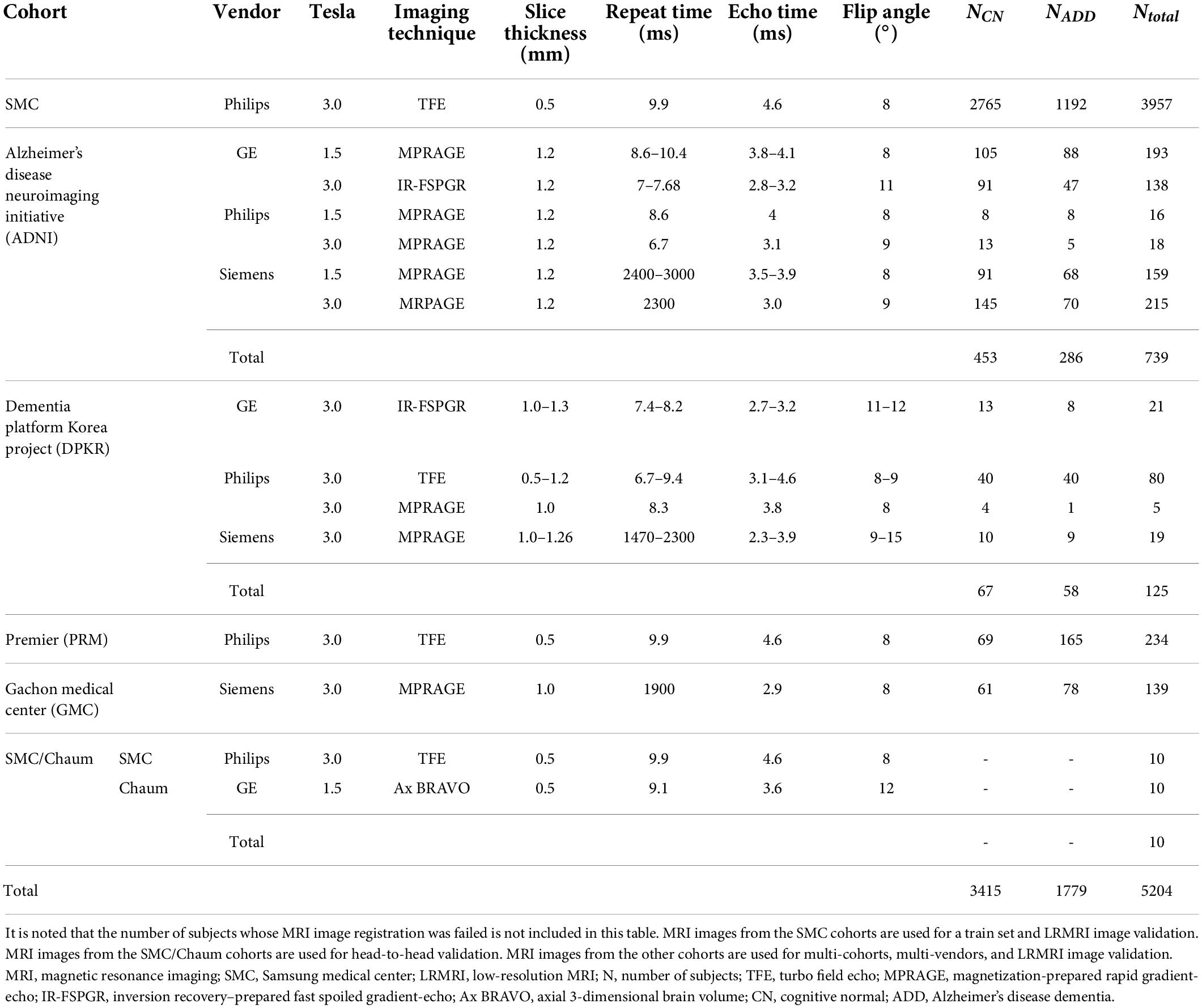
Table 1. The number of subjects used in this study.
The MRI images from the SMC cohort’s subjects were used for model training. MRI images from subjects belonging to the ADNI, DPKR, PRM, and GMC were used for external validation. Moreover, ten pairs of MRI images from subjects in the SMC/Chaum cohort were used for head-to-head validation.
Low-resolution magnetic resonance imaging image generation
Since most public MRI datasets consist of HRMRI images, we generated LRMRI images by downsampling axial slices of non-preprocessed original HRMRI images to perform LRMRI image validation. We sampled a maximum total of 25 slices in an axial plane containing cerebral from original HRMRI images with uniform intervals. Figure 1 shows the example of the input HRMRI image and the output LRMRI image. After downsampling, slice thickness becomes 0.5–1.25mm to 4.5–5.5mm, and the imaging plane was converted to an axial plane from the sagittal plane. We used the downsampled template and skull mask to preprocess downsampled images. After image preprocessing, we checked its quality and excluded 150 subjects due to registration failure. Table 2 shows the detailed information of the MRI images from subjects per diagnostics group, MRI scan protocol, and MRI scanner vendors.
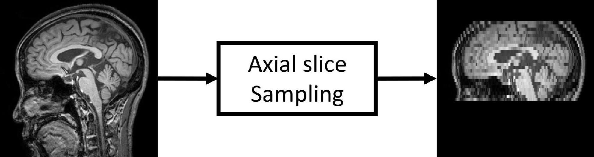
Figure 1. Low-resolution magnetic resonance imaging (LRMRI) image generation. LRMRI images were generated from high-resolution magnetic resonance imaging (HRMRI) images in this study by sampling a maximum total of 25 slices in an axial plane containing cerebral in uniform intervals. After sampling, the slice thickness becomes 0.5–1.25 mm to 4.5–5.5°mm.
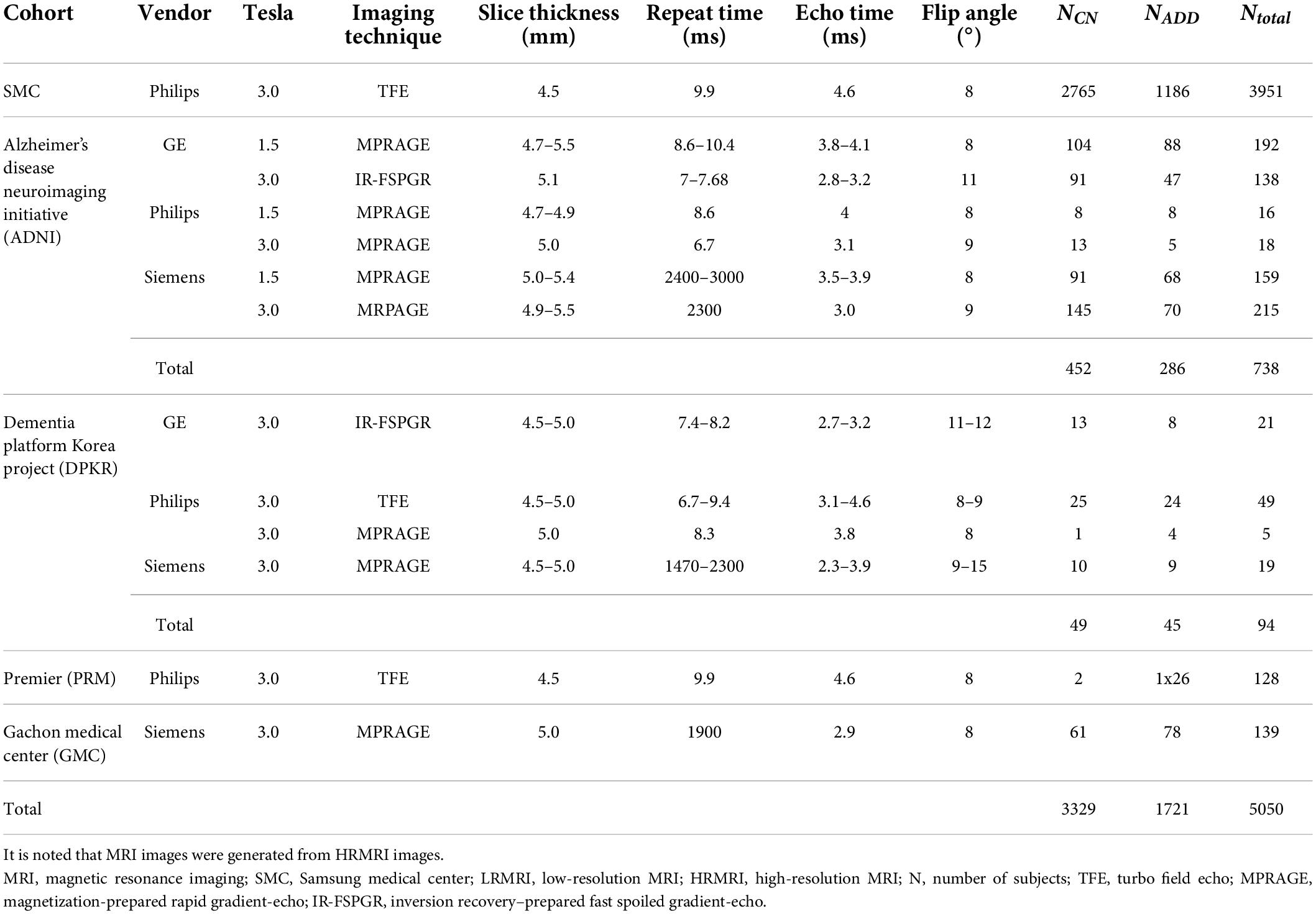
Table 2. The number of subjects whose low-resolution magnetic resonance imaging image registration was succeeded.
Image preprocessing
As shown in Figure 2, all MRI images including both HRMRI and LRMRI were first non-uniformly corrected using the N4ITK algorithm (Tustison et al., 2010) and non-linearly registered to MNI space using the Advanced Normalization Tools (ANTs) software package (Avants et al., 2009). After registration, all MRI images were skull stripped, and their intensity has trimmed by the sum of the mean intensity of the white matter (WM) mask and 2.5 times the standard deviation of the WM mask, where the WM mask was calculated using the fuzzy C-means clustering algorithm (Reinhold et al., 2019). Finally, MRI images were min-max normalized, and then three axial slices, including the hippocampus region, were extracted to use ImageNet pretrained weights.
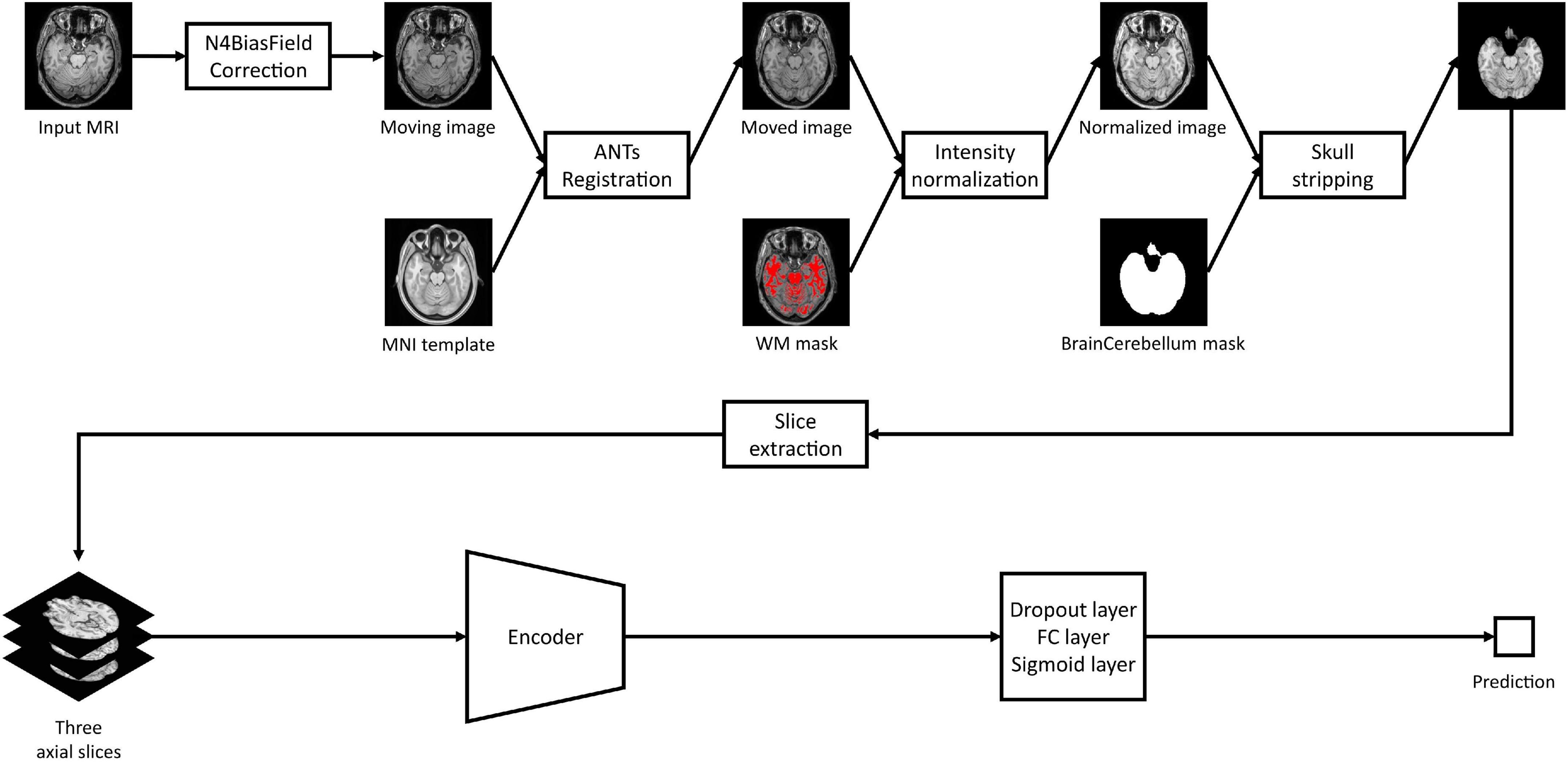
Figure 2. Study overview. Magnetic resonance imaging images are preprocessed with our preprocessing pipeline, and three axial slices including the hippocampus were extracted. The extracted slices are converted into scalar prediction by passing through the encoder, dropout, fully connected, and sigmoid layers.
Model development
We used the Inception Res Net V2 (Szegedy et al., 2017) architecture as a backbone since it is fast and lightweight and performs well. To access the effect of model developments, we trained five versions of the models, models A, B, C, D, and E, in which all of their encoders have the same input size of 130 × 130 × 3.
Model A is a vanilla Inception Res Net V2 model without a top. We added a dropout layer with a 0.2 dropout ratio, a fully connected layer with one output node, and a sigmoid activation layer at the end of model A. For model A, the three preprocessed slices were concatenated into a channel axis, encoded into a 1,536-dimensional vector, passed three layers, and created a scalar prediction which means the probability of ADD that can be used in classification when the threshold is applied. Model A structure would be a usual choice for researchers who plan to use pretrained weights. Model B is the same as model A except for MRI slice encoding. To encode enough information from each slice individually and combine them at a high level, we encoded each of the three axial slices from one subject and concatenate them before the fully connected layer. The three preprocessed slices were converted into a total of three individual three-channel images by duplicating its single-channel image three times. After converting, three images were encoded into three 1,536-dimensional vectors, concatenated into a 4,608-dimensional vector, and passed the three layers mentioned above. Model C is the same as model B except for its normalization layer. Instance normalization was used instead of batch normalization (Ioffe and Szegedy, 2015). Model D is the same as model C except for the training procedure. Mixup (Zhang et al., 2017) with its hyperparameter of 10 was used in model D. Model E is the same as model D except for the optimizing process. We used SAM when optimizing model E. As a result, A, B, and C each have their own structure and the same optimizing procedure, but C, D, and E all have the same structure and different optimizing procedures.
Also, ImageNet pretrained weights except for the normalization layers were adopted to speed up model training. We trained all models for 100 epochs with a batch size of 64, optimized through SGD optimizer with the momentum of 0.9, and label smoothing (Müller et al., 2019) with its hyperparameter of 0.1 using weighted binary cross-entropy loss. Left and right flip was performed for real-time data augmentation. For each of the five models, a 5-fold cross-validation was conducted with the SMC cohort. The SMC cohort’s MRI scans were randomly divided into five groups, four of which were used for training and the remaining for validation. For the random split, the random seed 0 was used. We saved weights with the best validation area under the receiver operating curve (AUC) at the end of an epoch for each fold. Then, we averaged the predictions of the models obtained by 5-fold cross-validation, from models A to E when evaluating the model with external cohorts.
All training was conducted using NVIDIA P100 GPUs with 16GB of memory per GPU, and all deep learning models were implemented using Tensorflow version 2.5.0 (Abadi et al., 2016) and Keras version 2.5.0 (Chollet, 2015).
The design of multi-scenario validation
We developed the following hypotheses concerning an ideal trustworthy MRI-based ADD classification model: an ideal reliable MRI-based ADD classification model would not have poor performance when given unseen protocol MRI, would be robust to scanner vendor differences, would be robust to LRMRI images, and would have the same prediction values when given MRI scans from the same subject at similar time points. We built multi-scenario validation to analyze how our models satisfy those hypotheses in various conditions.
Multi-cohort, multi-vendor, and low-resolution magnetic resonance imaging image validation
We designed multi-cohort validation with the ADNI, DPKR, PRM, and GMC cohorts. MRI images from the PRM cohort have the same protocol as the SMC cohort, while the other cohorts have different protocols. Thus, we evaluated the model’s reliability by comparing the two model’s performance in the ADNI, DPKR, and GMC cohorts. Also, we would interpret the effect of applied methods on the model’s classification performance by comparing the model’s performance to the PRM cohort.
Similarly, we designed multi-vendor validation with the GE, Philips, and Siemens vendor subgroups. For multi-vendor validation, we would interpret the effect of applied methods on the model’s reliability by comparing the two model’s performance on the GE and Siemens vendor subgroups. Also, we would interpret the effect of applied methods on the model’s classification performance by comparing the model’s performance on the Philips vendor subgroup.
To evaluate the model’s performance on LRMRI images, we designed LRMRI image validation with the generated LRMRI images. We repeated multi-cohort validation and multi-vendor validation with LRMRI images. It is noted that the input image’s size is not changed from 130 × 130 × 3 when evaluating the models on LRMRI images.
Two metrics were used to assess performance: AUC and classification accuracy. The classification accuracy was determined using Youden’s J statistics (Youden, 1950), which determines the cutoff point for the maximum summation value of specificity and sensitivity.
Head-to-head validation
To explore the reproducibility of the model at the subject level, we performed head-to-head validation with the SMC/Chaum cohort. Subjects in the SMC/Chaum have paired MRI images: one is from the SMC and the other one is from the Chaum, and the mean time interval between the two scans was 300°days. We calculated two metrics, namely, Δprediction and slope,
where predictionSMC = the model’s prediction of the images scanned from the SMC; predictionChaum = the model’s prediction of the images scanned from the Chaum; i = the index of the subject; and α = the value obtained from the slope of the linear regression equation of the model’s predictions. We could interpret a model with a smaller Δprediction value, and a bigger slope value would be more reliable.
Results
Cross-validation
The mean AUC and the mean classification accuracy across 5-fold are plotted in Figure 3, the blue line. The performance gap was the biggest between model A and model B, respectively, 0.0093 and 0.024 for the mean AUC and classification accuracy. From model B to model E, the gap was relatively small.
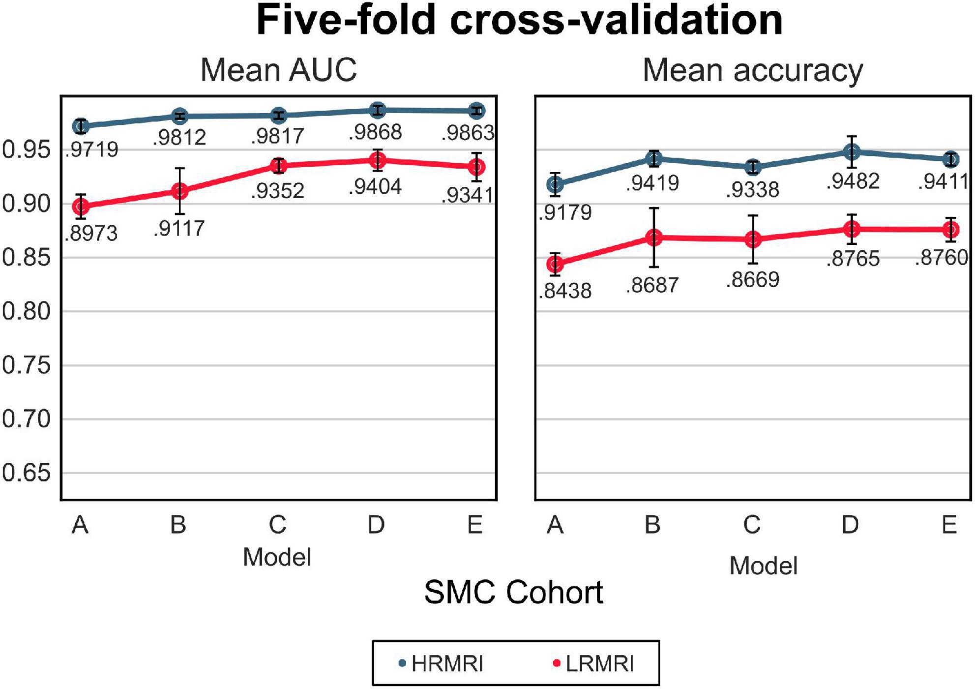
Figure 3. The 5-fold cross-validation and low-resolution magnetic resonance imaging image validation with the samsung medical center cohort. The blue line indicates the result of the high-resolution magnetic resonance imaging images, while the red line indicates the result of the LRMRI images. Models: A = vanilla inception res net V2; B = same with A except for slice encoding. Instead of encoding three slices at once, each of the three is encoded; C = same with B except for the normalization layer. Instead of batch normalization, the instance normalization layer was used; D = same with C except for the training procedure. Mixup with its hyperparameter value of 10 was used; E = same with D except for the optimizing process. Sharpness-aware minimization was used. SMC, Samsung medical center; HRMRI, high-resolution magnetic resonance imaging; LRMRI, low-resolution magnetic resonance imaging.
Exploring the effect of modification on reliability via multi-scenario validation
We assessed our five models with multi-scenario validation. Since the models are the same as adjacent versions of the models except for one option, we explored the effect of model modifications on reliability by comparing two adjacent versions of the models, e.g., model B and model C are the same but differ in their normalization layers. By comparing two adjacent models, for example, we can assess the effect of the instance normalization vs. the batch normalization.
Multi-cohort, multi-vendor, and low-resolution magnetic resonance imaging image validation
The AUC and classification accuracy for four cohorts are plotted in Figure 4, the blue line. Moreover, the AUC and classification accuracy for three vendor subgroups is plotted in Figure 5, blue line. The overall AUC and classification accuracy increases from model A to model E for all cohorts and vendor subgroups, which means that the modifications enhanced the model’s classification performance. This implies that the modifications are not only successful in the perspective of the model’s classification performance but also successful in the perspective of the model’s reliability.
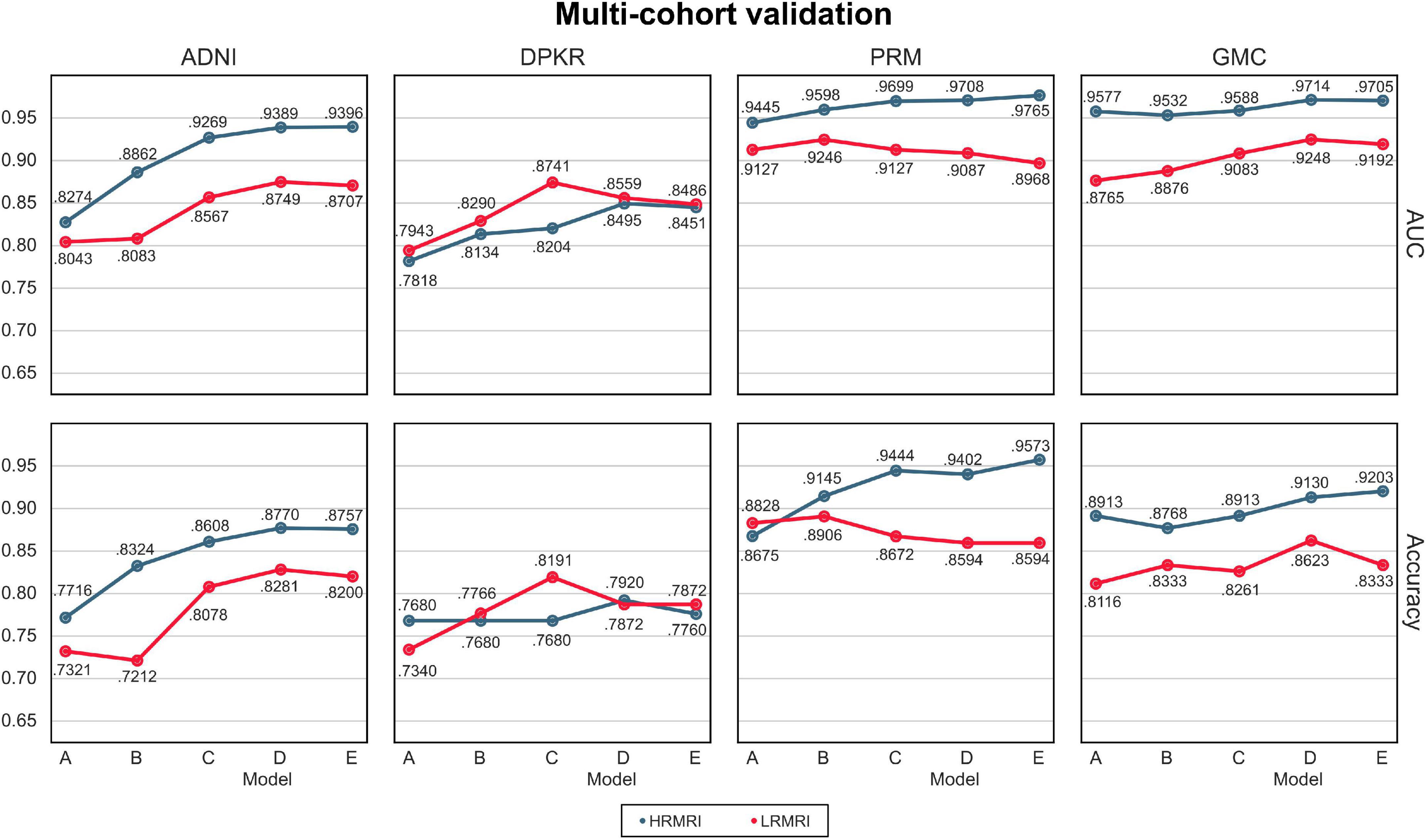
Figure 4. Multi-cohorts and low-resolution magnetic resonance imaging image validation. All the results are calculated by averaging the predictions of the models obtained from 5-fold cross-validation. The blue line indicates the result of the high-resolution magnetic resonance imaging images, while the red line indicates the result of the LRMRI images. Models: A = vanilla inception res net V2; B = same with A except for slice encoding. Instead of encoding three slices at once, each of the three is encoded; C = same with B except for the normalization layer. Instead of batch normalization, the instance normalization layer was used; D = same with C except for the training procedure. Mixup with its hyperparameter value of 10 was used; E = same with D except for the optimizing process. Sharpness-aware minimization was used. ADNI, Alzheimer’s Disease Neuroimaging Initiative; DPKR, Dementia Platform Korea project; PRM, Premier; GMC, Gachon medical center; HRMRI, high-resolution magnetic resonance imaging; LRMRI, low-resolution magnetic resonance imaging.
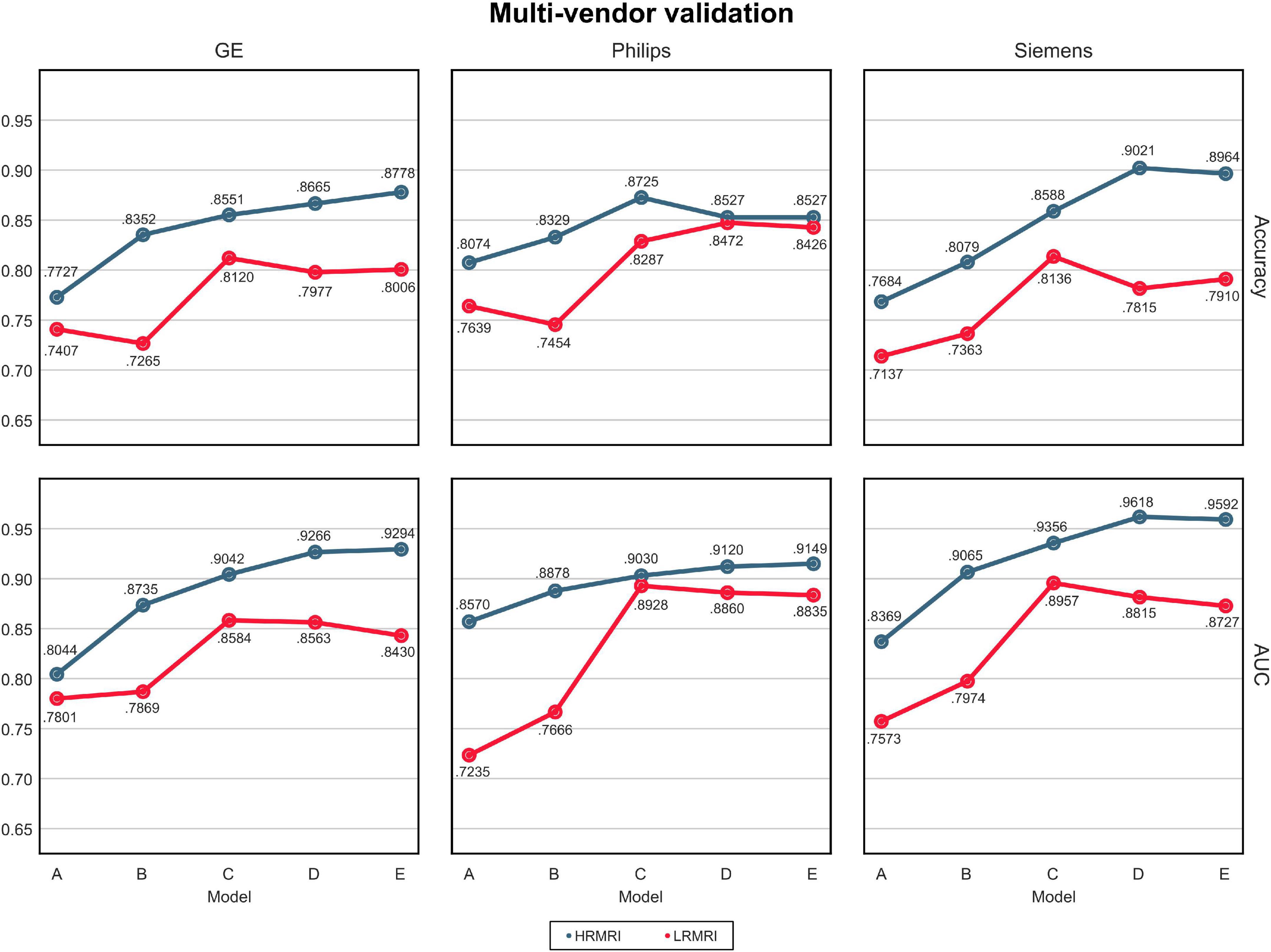
Figure 5. Multi-vendors and low-resolution magnetic resonance imaging image validation. The values in this figure were calculated by averaging the predictions of the models obtained from 5-fold cross-validation. The blue line indicates the result of the high-resolution magnetic resonance imaging, while the red line indicates the result of the LRMRI. Models: A = vanilla inception res net V2; B = same with A except for slice encoding. Instead of encoding three slices at once, each of the three is encoded; C = same with B except for the normalization layer. Instead of batch normalization, the instance normalization layer was used; D = same with C except for the training procedure. Mixup with its hyperparameter value of 10 was used; E = same with D except for the optimizing process. Sharpness-aware minimization was used. HRMRI, high-resolution magnetic resonance imaging; LRMRI, low-resolution magnetic resonance imaging.
For the LRMRI image validation, the mean AUC and the mean classification accuracy across 5-fold are plotted in Figure 3, the red line. It is noted that we trained the models with only HRMRI images. In this study, it is hard to tell which models C, D, or E classify LRMRI better.
For multi-cohort validation, the results are plotted in Figure 4, the red line. In addition, for multi-vendor validation, the results are plotted in Figure 5, the red line. In this study, the overall tendency follows the above multi-cohort validations without the PRM cohort since the generated LRMRI images in the PRM cohort are poor-balanced: the PRM cohort contains only two LRMRI images for the CN subjects. The overall tendency in the multi-vendor validation also follows the multi-vendor validation performed above.
Head-to-head validation
The Δprediction, slope, and the prediction score of each subject per model are plotted in Figure 6. The x-axis is the model’s prediction score of the SMC scans, while the y-axis is for the Chaum scans. From models A to E, Δprediction decreases, and slope increases, meaning that the modifications enhanced the model’s reliability.
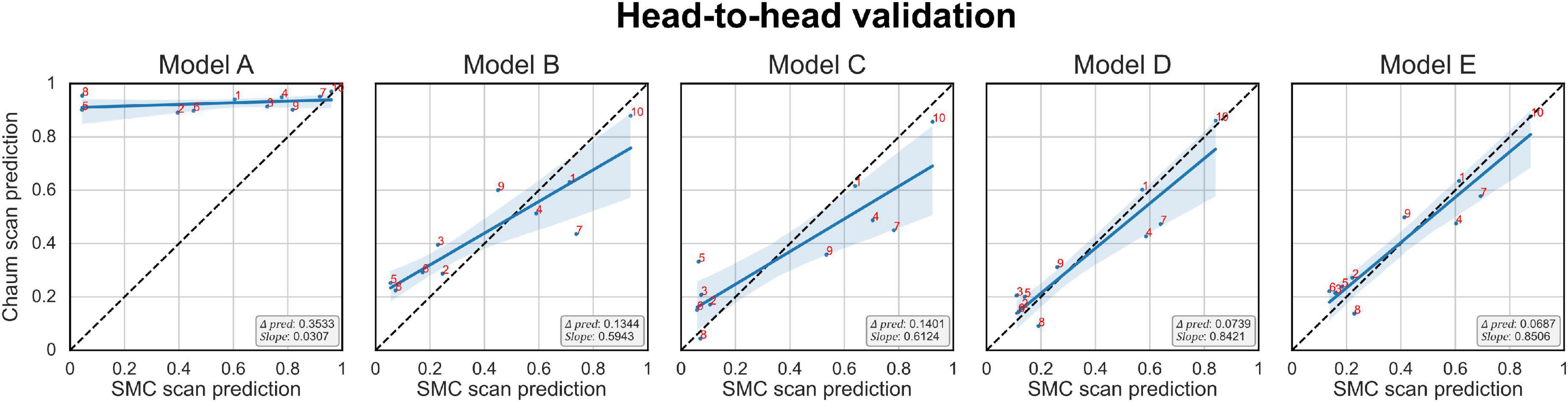
Figure 6. Head-to-head validation. The black dotted line indicates y = x. Subjects in the SMC/Chaum cohort have undergone two magnetic resonance imaging scans, one at the SMC and the other at the Chaum. The x-axis represents the averaged predictions of the SMC scans from the models obtained from 5-fold cross-validation, while the y-axis represents the averaged predictions of the Chaum scans from the models obtained from 5-fold cross-validation. Δpred is the mean of the absolute value of the difference between the predictions for the SMC scans and the Chaum scans. The slope is the smaller of the two values, α and , where α is the value obtained from the slope of the linear regression equation of the predictions from the SMC scans and the Chaum scans. The blue line indicates the result of linear regression. The smaller Δpred and the bigger slope are better. Models: A = vanilla inception res net V2; B = same with A except for slice encoding. Instead of encoding three slices at once, each of the three is encoded; C = same with B except for the normalization layer. Instead of batch normalization, the instance normalization layer was used; D = same with C except for the training procedure. Mixup with its hyperparameter value of 10 was used; E = same with D except for the optimizing process. Sharpness-aware minimization was used. SMC, Samsung medical center.
Discussion
In this study, we constructed an MRI-based ADD classification CNN model using individual slice encoding, instance normalization, Mixup, and SAM and showed that the model’s reliability could be improved by adopting those methods. We further validated the efficacy of the proposed model using comprehensive multi-scenarios: multi-protocols, multi-vendors, LRMRI image, and head-to-head validation that are critical in the usage of our tool in the real-world clinical field.
Via multi-scenario validation, we extensively investigated the effect of each option in terms of reliability across heterogeneous environments: (1) the individual slice encoding method improved the model’s performance in various experimental settings. The individual slice encoding method integrates information at a higher level, thereby the model can extract more reliable information related to ADD and avoid overfitting, and (2) the instance normalization method increased the model’s reliability by learning invariant features to different styles (Pan et al., 2018). In our problem setting, the features learned by different styles could be related to different MRI scan protocols. Therefore, the instance normalization technique makes our model robust against different MRI protocols, and (3) the Mixup method sometimes failed to improve the model’s performance on LRMRI if augmented data are different from test data. But it improved the model’s performance in most cases by generating a convex combination of the input samples, which would approximate various intermediate stages of disease progression, and (4) the SAM technique failed to improve the model’s performance on LRMRI when the sharp minima which skipped to find the flat minima performed better in test data than flat minima. However, it increased the model’s reliability in most cases by finding weights that are more robust to distributional shifts, which might be related to heterogeneous MRI scan protocols.
We compared the performance of the proposed method with other previous deep learning-based ones (Table 3). The data used for training or validation are different from each other, so it is not comfortable to directly compare the performance in detail. Nevertheless, we can see that our model E achieved comparable performance with other studies, even though our model E had not seen protocols in the ADNI cohort during the training process.
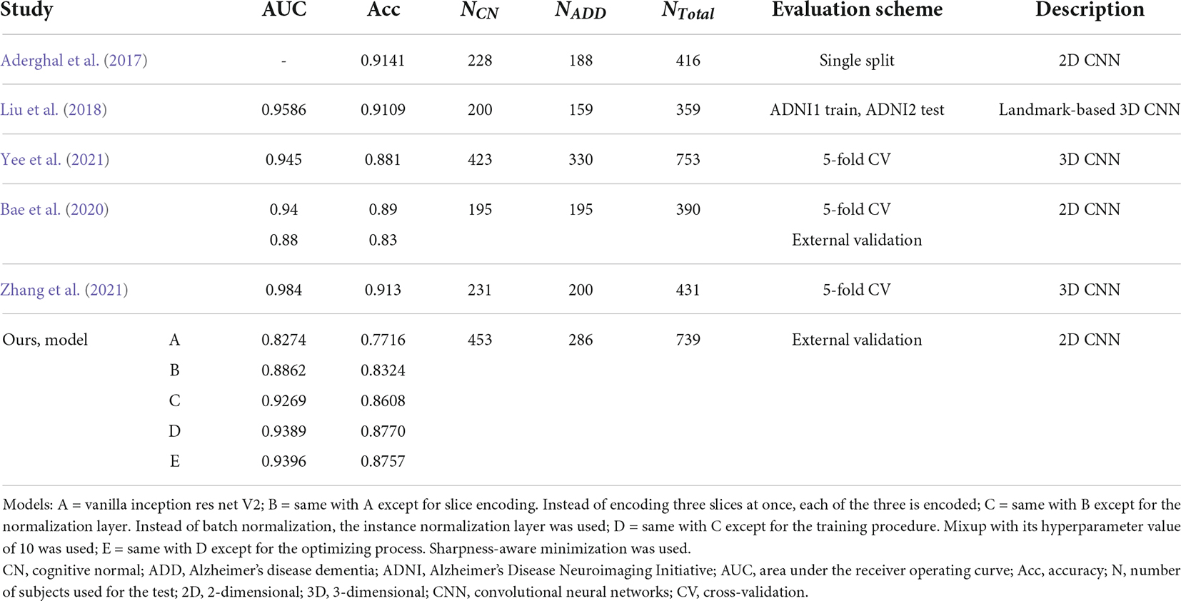
Table 3. Comparison of published cognitive normal vs. Alzheimer’s disease dementia classification performances in the Alzheimer’s disease neuroimaging initiative cohort.
Our LRMRI image validation has limitations since the generated LRMRI images were used as the surrogate of the original LRMRI images. Nevertheless, the performance could be meaningful because it used an image that reflects low resolution in its axial axis of LRMRI images, a significant difference between LRMRI image and HRMRI image.
In conclusion, we showed that we could improve a CNN model’s reliability with a small computational cost by adopting minor modifications to the existing deep learning model, which was then extensively validated through multiple scenarios. The proposed method would be worth applying to researchers who want to conduct CNN-based ADD diagnostic research in various experimental settings. Our study can potentially be improved further by designing additional real-world encounterable validation scenarios.
Data availability statement
The datasets generated and/or analyzed for this study are available from the corresponding author, Prof. J-KS on reasonable request. Requests to access these datasets should be directed to jkseong@korea.ac.kr.
Ethics statement
Ethical review and approval was not required for the study on human participants in accordance with the local legislation and institutional requirements. The patients/participants provided their written informed consent to participate in this study.
Author contributions
Y-HS and J-YY derived the experimental results using the data. Y-HS proceeded to interpret the results of the experiment and wrote the manuscript. J-KS contributed to the interpretation and progress of the study as the corresponding author. YN, HJ, SS, and DN contributed to data curation. All authors contributed to the article and approved the submitted version.
Funding
This research was supported by the National Research Foundation of Korea (NRF) grant funded by the Korea government (No. 2022R1A4A1033856). This study was supported by a grant of the Korea Healthcare Technology R&D Project through the Korea Health Industry Development Institute (KHIDI) and funded by the Ministry of Health & Welfare, Republic of Korea (Grant No: HI14C1135).
Conflict of interest
The authors declare that the research was conducted in the absence of any commercial or financial relationships that could be construed as a potential conflict of interest.
Publisher’s note
All claims expressed in this article are solely those of the authors and do not necessarily represent those of their affiliated organizations, or those of the publisher, the editors and the reviewers. Any product that may be evaluated in this article, or claim that may be made by its manufacturer, is not guaranteed or endorsed by the publisher.
References
Abadi, M., Barham, P., Chen, J., Chen, Z., Davis, A., Dean, J., et al. (2016). “Tensorflow: A system for large-scale machine learning,” in Proceedings of the 12th {USENIX} Symposium on Operating Systems Design and Implementation ({OSDI} 16) (Savannah), 265–283.
Aderghal, K., Benois-Pineau, J., and Afdel, K. (2017). “Classification of sMRI for Alzheimer’s disease diagnosis with CNN: Single siamese networks with 2D+? Approach and fusion on ADNI,” in Proceedings of the 2017 ACM on international conference on multimedia retrieval, Bucharest, 494–498.
Avants, B. B., Tustison, N., and Song, G. (2009). Advanced normalization tools (ANTS). Insight J. 2, 1–35. doi: 10.1007/s11682-020-00319-1
Bae, J. B., Lee, S., Jung, W., Park, S., Kim, W., Oh, H., et al. (2020). Identification of Alzheimer’s disease using a convolutional neural network model based on T1-weighted magnetic resonance imaging. Sci. Rep. 10, 1–10. doi: 10.1038/s41598-020-79243-9
Cho, Y., Seong, J.-K., Jeong, Y., Shin, S. Y., and Initiative, A. S. D. N. (2012). Individual subject classification for Alzheimer’s disease based on incremental learning using a spatial frequency representation of cortical thickness data. Neuroimage 59, 2217–2230. doi: 10.1016/j.neuroimage.2011.09.085
Chung, J., Yoo, K., Lee, P., Kim, C. M., Roh, J. H., Park, J. E., et al. (2017). Normalization of cortical thickness measurements across different T1 magnetic resonance imaging protocols by novel W-score standardization. Neuroimage 159, 224–235. doi: 10.1016/j.neuroimage.2017.07.053
Deng, J., Dong, W., Socher, R., Li, L.-J., Li, K., and Fei-Fei, L. (2009). “Imagenet: A large-scale hierarchical image database,” in Proceedings of the 2009 IEEE Conference on Computer Vision and Pattern Recognition (Miami, FL: IEEE), 248–242. doi: 10.1109/TMI.2016.2528162
Foret, P., Kleiner, A., Mobahi, H., and Neyshabur, B. (2020). Sharpness-aware minimization for efficiently improving generalization. arXiv [Preprint]. doi: 10.48550/arXiv.2010.01412
Fortin, J.-P., Cullen, N., Sheline, Y. I., Taylor, W. D., Aselcioglu, I., Cook, P. A., et al. (2018). Harmonization of cortical thickness measurements across scanners and sites. Neuroimage 167, 104–120.
Gray, K. R., Aljabar, P., Heckemann, R. A., Hammers, A., Rueckert, D., and Initiative, A. S. D. N. (2013). Random forest-based similarity measures for multi-modal classification of Alzheimer’s disease. Neuroimage 65, 167–175. doi: 10.1016/j.neuroimage.2012.09.065
Han, X., Jovicich, J., Salat, D., Van Der Kouwe, A., Quinn, B., Czanner, S., et al. (2006). Reliability of MRI-derived measurements of human cerebral cortical thickness: The effects of field strength, scanner upgrade and manufacturer. Neuroimage 32, 180–194. doi: 10.1016/j.neuroimage.2006.02.051
Huang, X., and Belongie, S. (2017). “Arbitrary style transfer in real-time with adaptive instance normalization,” in Proceedings of the IEEE International Conference on Computer Vision (Venice: IEEE), 1501–1510.
Ioffe, S., and Szegedy, C. (2015). “Batch normalization: Accelerating deep network training by reducing internal covariate shift,” in Proceedings of the 32nd International Conference on Machine Learning: PMLR, Lille, 448–456. doi: 10.1007/s11390-020-0679-8
Liu, M., Zhang, J., Adeli, E., and Shen, D. (2018). Landmark-based deep multi-instance learning for brain disease diagnosis. Med. Image Anal. 43, 157–168. doi: 10.1016/j.media.2017.10.005
Ma, D., Popuri, K., Bhalla, M., Sangha, O., Lu, D., Cao, J., et al. (2019). Quantitative assessment of field strength, total intracranial volume, sex, and age effects on the goodness of harmonization for volumetric analysis on the ADNI database. Hum. Brain Mapp. 40, 1507–1527. doi: 10.1002/hbm.24463
Magnin, B., Mesrob, L., Kinkingnéhun, S., Pélégrini-Issac, M., Colliot, O., Sarazin, M., et al. (2009). Support vector machine-based classification of Alzheimer’s disease from whole-brain anatomical MRI. Neuroradiology 51, 73–83. doi: 10.1007/s00234-008-0463-x
Mårtensson, G., Ferreira, D., Granberg, T., Cavallin, L., Oppedal, K., Padovani, A., et al. (2020). The reliability of a deep learning model in clinical out-of-distribution MRI data: A multicohort study. Med. Image Anal. 66:101714. doi: 10.1016/j.media.2020.101714
Müller, R., Kornblith, S., and Hinton, G. (2019). When does label smoothing help? arXiv [Preprint]. doi: 10.48550/arXiv.1906.02629
Pan, X., Luo, P., Shi, J., and Tang, X. (2018). “Two at once: Enhancing learning and generalization capacities via ibn-net,” in Proceedings of the European Conference on Computer Vision (ECCV), Munich, 464–479.
Reinhold, J. C., Dewey, B. E., Carass, A., and Prince, J. L. (2019). “Evaluating the impact of intensity normalization on MR image synthesis,” in Proceedings of the Medical Imaging 2019: Image Processing: International Society for Optics and Photonics (San Diego, CA), 109493H.
Schnack, H. G., Van Haren, N. E., Brouwer, R. M., Van Baal, G. C. M., Picchioni, M., Weisbrod, M., et al. (2010). Mapping reliability in multicenter MRI: Voxel-based morphometry and cortical thickness. Hum. Brain Mapp. 31, 1967–1982. doi: 10.1002/hbm.20991
Szegedy, C., Ioffe, S., Vanhoucke, V., and Alemi, A. A. (2017). “Inception-v4, inception-resnet and the impact of residual connections on learning,” in Proceedings of the Thirty-first AAAI Conference on Artificial Intelligence (Mountain View, CA: Google Inc).
Tustison, N. J., Avants, B. B., Cook, P. A., Zheng, Y., Egan, A., Yushkevich, P. A., et al. (2010). N4ITK: Improved N3 bias correction. IEEE Trans. Med. Imaging 29, 1310–1320.
Ulyanov, D., Vedaldi, A., and Lempitsky, V. (2016). Instance normalization: The missing ingredient for fast stylization. arXiv [Preprint] arXiv: 1607.08022.
Yee, E., Ma, D., Popuri, K., Wang, L., Beg, M. F., and Initiative, A. S. D. N. (2021). Construction of MRI-based Alzheimer’s disease score based on efficient 3D convolutional neural network: Comprehensive validation on 7,902 images from a multi-center dataset. J. Alzheimers Dis. 79, 47–58. doi: 10.3233/JAD-200830
Zhang, H., Cisse, M., Dauphin, Y. N., and Lopez-Paz, D. (2017). Mixup: Beyond empirical risk minimization. arXiv [Preprint]. doi: 10.48550/arXiv.1710.09412
Zhang, X., Han, L., Zhu, W., Sun, L., and Zhang, D. (2021). An explainable 3D Residual self-attention deep neural network for joint atrophy localization and Alzheimer’s disease diagnosis using structural MRI. IEEE J. Biomed. Health Inform. 1–1. https://ieeexplore.ieee.org/abstract/document/9381587?casa_token=4_95CeCwfXEAAAAA:0mjBrPzVCjqu77_qewRgBnhBSxWrriANfDJxXuHYSCQKh67k_dlmss17q2xSuvm9MKOSD-zXY20 doi: 10.1109/JBHI.2021.3066832
Keywords: Alzheimer’s disease, multi-cohort validation, structural magnetic resonance imaging, deep learning, reliability, clinical application, low-resolution magnetic resonance imaging
Citation: Song Y-H, Yi J-Y, Noh Y, Jang H, Seo SW, Na DL and Seong J-K (2022) On the reliability of deep learning-based classification for Alzheimer’s disease: Multi-cohorts, multi-vendors, multi-protocols, and head-to-head validation. Front. Neurosci. 16:851871. doi: 10.3389/fnins.2022.851871
Received: 10 January 2022; Accepted: 27 July 2022;
Published: 07 September 2022.
Edited by:
Jorge Sepulcre, Massachusetts General Hospital and Harvard Medical School, United StatesReviewed by:
Arnav Bhavsar, Indian Institute of Technology Mandi, IndiaPramod Kumar Pisharady, University of Minnesota, United States
Copyright © 2022 Song, Yi, Noh, Jang, Seo, Na and Seong. This is an open-access article distributed under the terms of the Creative Commons Attribution License (CC BY). The use, distribution or reproduction in other forums is permitted, provided the original author(s) and the copyright owner(s) are credited and that the original publication in this journal is cited, in accordance with accepted academic practice. No use, distribution or reproduction is permitted which does not comply with these terms.
*Correspondence: Joon-Kyung Seong, jkseong@korea.ac.kr
†Data used in preparation of this article were obtained from the Alzheimer’s Disease Neuroimaging Initiative (ADNI) database (adni.loni.usc.edu). As such, the investigators within the ADNI contributed to the design and implementation of ADNI and/or provided data but did not participate in analysis or writing of this report. A complete listing of ADNI investigators can be found at: http://adni.loni.usc.edu/wp-content/uploads/how_to_apply/ADNI_Acknowledgement_List.pdf