 Giacomo Innocenti
 Mauro Di Marco2
- 1Dipartimento di Ingegneria dell'Informazione, Università degli Studi di Firenze, Firenze, Italy
- 2Dipartimento di Ingegneria dell'Informazione e Scienze Matematiche, Università degli Studi di Siena, Siena, Italy
Since the introduction of memristors, it has been widely recognized that they can be successfully employed as synapses in neuromorphic circuits. This paper focuses on showing that memristor circuits can be also used for mimicking some features of the dynamics exhibited by neurons in response to an external stimulus. The proposed approach relies on exploiting multistability of memristor circuits, i.e., the coexistence of infinitely many attractors, and employing a suitable pulse-programmed input for switching among the different attractors. Specifically, it is first shown that a circuit composed of a resistor, an inductor, a capacitor and an ideal charge-controlled memristor displays infinitely many stable equilibrium points and limit cycles, each one pertaining to a planar invariant manifold. Moreover, each limit cycle is approximated via a first-order periodic approximation analytically obtained via the Describing Function (DF) method, a well-known technique in the Harmonic Balance (HB) context. Then, it is shown that the memristor charge is capable to mimic some simplified models of the neuron response when an external independent pulse-programmed current source is introduced in the circuit. The memristor charge behavior is generated via the concatenation of convergent and oscillatory behaviors which are obtained by switching between equilibrium points and limit cycles via a properly designed pulse timing of the current source. The design procedure takes also into account some relationships between the pulse features and the circuit parameters which are derived exploiting the analytic approximation of the limit cycles obtained via the DF method.
1. Introduction
The ever-growing need of computing power to handle data intensive applications is seriously challenging conventional digital von Neumann computing architectures (Bonomi et al., 2012; Satyanarayanan, 2017; Williams, 2017). The physical separation between the computing and memory units can indeed generate long latency time and large energy consumption when data intensive tasks are performed. In this context, researchers look at the emerging nanoscale analog devices, such as memristors, as a viable approach for developing new computing paradigms, based on in-memory and analog computation, which are potentially capable to overcome the limitations of conventional computer architectures (Waldrop, 2016; Zidan et al., 2018; Krestinskaya et al., 2020).
The memristor (a shorthand for memory resistor) is the fourth basic passive circuit element theoretically introduced by Prof. Leon Chua in 1971 (Chua, 1971). The appealing features of a memristor are non-volatility, i.e., the memristor capability to hold data in memory without the need of a power supply, and non-linearity, which makes memristor circuits capable to generate quite a rich variety of oscillatory and complex dynamics. The combination of these two features enables in-memory computing, i.e., the co-location of computation and memory in the same device (Ielmini and Wong, 2018). In-memory computing, which resembles a basic principle of brain computation, can provide several advantages, such as low energy consumption, high bandwidths, excellent scalability, thus lending itself as quite a promising novel computing approach in the field of artificial intelligence and big data (Ielmini and Pedretti, 2020). Memristor circuits have been already positively used to address several tasks, including the solution of global optimization, constraint satisfaction and linear algebra problems (Yang et al., 2013; Wang et al., 2015; Kumar et al., 2017). They are also used as building blocks in reservoir computing systems (Du et al., 2017) and neuromorphic computing for on-line signal processing tasks (Di Marco et al., 2016, 2017; Di Marco et al., 2017; Ascoli et al., 2020a,b).
Since the very beginning it was clear that understanding the peculiar dynamical features of memristor circuits is the key step for developing analog in-memory computing schemes. It has been definitely shown that memristor circuits are capable to generate quite a large variety of dynamical behaviors (Corinto et al., 2011; Corinto et al., 2019; Pershin and Di Ventra, 2011; Xu et al., 2016; Yuan et al., 2016; Di Marco et al., 2018), including bursting oscillations (see e.g., Wang et al., 2019 and references therein). Recently, a new technique, named flux-charge analysis method (FCAM), has been introduced for the analysis of memristor circuits in the flux-charge domain (Corinto and Forti, 2016, 2017, 2018). FCAM permits to show that the dynamical richness displayed by memristor circuits is a consequence of the property that the state space of any given circuit, i.e., with its parameter having fixed values, contains infinitely many invariants manifolds (foliation property of the state space). This specific property implies that in memristor circuits there is the coexistence of infinitely many different attractors, a property referred to as multistability. Moreover, structural changes of the attractors are observed when the initial conditions are varied while keeping constant the values of the circuit parameters, a peculiar phenomenon which is referred to as bifurcations without parameters (Corinto and Forti, 2017; Di Marco et al., 2018; Innocenti et al., 2019b). In particular, Di Marco et al. (2018), Innocenti et al. (2019b) have employed techniques within the Harmonic Balance (HB) context for predicting limit cycles and their bifurcations by first showing that the dynamics of the memristor circuit admits an equivalent input-output representation, which has been recently extended also to circuits containing memory elements (Innocenti et al., 2020).
Among other applications, it has been soon recognized that memristors can be successfully employed as synapses in neuromorphic circuits (see e.g., Jo et al., 2010; Adhikari et al., 2012; Thomas, 2013; Kim et al., 2015; Hu et al., 2016; Hong et al., 2019). It has been also pointed out that memristor circuits appear to be suited for modeling some features of the dynamics of neurons. Some contributions provide a memristor representation of popular neuron models (see e.g., Chua et al., 2012; Usha and Subha, 2019 for the Hodgkin-Huxley axon), while others show how to mimic some typical dynamics displayed by cortical neurons (see e.g., Babacan et al., 2016; Nakada, 2019, and references therein). In Innocenti et al. (2019a), it is shown that dynamics of the memristor Murali-Lakshmanan-Chua circuit, equipped with an independent pulse programmed input source and simple comparator and hysteresis feedback blocks, can resemble some dynamical behaviors of cortical neurons. Finally, it is worth noting that HB techniques have been suitably employed for the analysis of neural oscillations (see e.g., Chen et al., 2008; Matsuoka, 2011 and references therein).
The purpose of this paper is to show how memristor circuits can be exploited for modeling some features of the neurons dynamics (see e.g., Izhikevich, 2000, 2007). The basic ideas are to exploit multistability, i.e., the fact that a memristor circuit contains infinitely many attractors (equilibria, limit cycles, …), and to employ a suitable pulse-programmed input for controlling multistability, i.e., for switching among the different attractors. Controlling multistability is currently a research field of general interest (see e.g., Pisarchik and Feudel, 2014 and references therein) and some contributions to the problem of steering the memristor circuit dynamics toward the attractors contained in one of the invariant manifolds have been given (Chen et al., 2018; Corinto and Forti, 2018; Corinto et al., 2019; Di Marco et al., 2019, 2020a,b). In particular, Di Marco et al. (2020b,a), Di Marco et al. (2021) have shown that the dynamics of a second order R, L, C circuit connected with a charge-controlled memristor can be steered, via a pulse programmed source, toward a pre-assigned invariant manifold where it converges toward the attractor contained in the manifold itself. In this paper, such a simple memristor circuit is used to mimic some aspects of the dynamics displayed by cortical neurons in response to an external stimulus. Section 2 describes the circuit and formulates the problem of interest. Specifically, the memristor charge should exhibit some typical neuron dynamics when the current source is suitably pulse-programmed. It is assumed that the pulses and their timing are generated by some given hardware mechanisms, whose design is not the object of the paper. Section 2 also illustrates the foliation property of the circuit state space in the input-less case, by characterizing the infinitely many invariant manifolds and the differential equations governing the dynamics onto them. Section 3 investigates the dynamics of the input-less circuit by showing that each manifold contains as attractor either a stable equilibrium point or a stable limit cycle. The limit cycles analysis is performed via the Describing Function (DF) method, a classical technique within the HB context. By exploiting the coexistence of stable equilibrium points and limit cycles and the knowledge of the first order periodic approximations, section 4 provides a procedure for the design of a pulse timing of the current source ensuring that the memristor charge mimics some dynamical features of the neuron response. The sought behavior of the memristor charge is obtained via a suitable concatenation of convergent and oscillatory behaviors, which are generated by switching between different attractors according to the designed pulse timing. The relation between the pulse timing parameters and the circuit parameters is also discussed. Some conclusions are finally drawn in section 5.
2. Problem Formulation and Preliminaries
The aim of the paper is to show that the coexistence of many different attractors in memristor circuits permits to mimic some features of the dynamics of cortical neurons. Specifically, we consider the simple circuit depicted in Figure 1 which contains a resistor R, an inductor L, a capacitor C and a non-linear charge-controlled memristor.
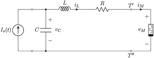
Figure 1. Charge-controlled memristor circuit with R, L,C components and independent current source Is.
The capacitor voltage, the inductor current, the memristor voltage and current are denoted by vC, iL, vM, and iM, respectively. The circuit is subject to an independent current source Is, which is the input of the circuit. The charge-flux characteristic of the memristor relating the charge qM and the flux φM is assumed to have both a linear and a cubic term. Specifically,
where the constant terms s0 and s1 satisfy
Throughout the paper, we assume that all the circuit parameters R, L, C, s0, s1 have normalized values. Also, we consider arbitrary units for the time.
We want to show that the circuit is able to generate some characteristic dynamical behaviors of a neuron in response to a pulse stimulus, as the typical one depicted in Figure 2A. Specifically, the memristor charge qM should display the time behavior of Figure 2B when the input source Is provides a suitable stimulus.
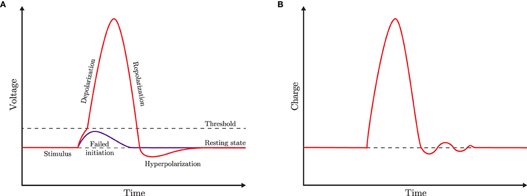
Figure 2. (A) Schematic of an ideal voltage-pulse of the cellular membrane (action potential). (B) Reference shape of the memristor charge-pulse considered in this paper. For the sake of simplicity, the depolarization is assumed to occur without distinction between the sub- and the super-threshold branches, and the hyperpolarization dynamics admits small ripples during the convergence to the resting state.
It can be readily verified that the circuit dynamics is described by the following third-order system of differential equations
where is the time-derivative operator1 and vC, qM, and iL are the state variables.
Let us consider the input-less case, i.e., Is = 0. It has been shown (see e.g., Corinto and Forti, 2017) that memristor circuits enjoy the so-called foliation property, i.e., the memristor state space is decomposed into infinitely many invariant manifolds. The verification of this property for the considered circuit is readily obtained. Since Is = 0, the first equation of Equation (3) can be rewritten equivalently as
which means that the quantity qM(t) + CvC(t) is constant along the solutions of Equation (3) with initial conditions vC(t0), qM(t0), and iL(t0) at time t = t0, i.e.,
Hence, in the input-less case the state space of the memristor circuit is decomposed into infinitely many invariant manifolds of the form
where Q0 is the index of the manifold whose value depends on the circuit initial conditions according to the relation Q0 = qM(t0) + CvC(t0). Note that the invariant manifolds M(Q0) are planar surfaces parameterized by the manifold index Q0, as illustrated in Figure 3.
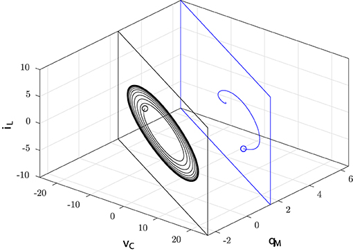
Figure 3. Invariant manifolds of the input-less circuit: the state space trajectory generated by the solution of Equation (3) with initial conditions vC(t0), qM(t0), iL(t0) (marked with ◦) at time t = t0 belongs to the manifold M(Q0) with Q0 = qM(t0) + CvC(t0) for all t ≥ t0.
We have then established that in the input-less case the circuit dynamics is confined to lie onto one of the invariant manifolds. The differential equations governing the dynamics onto the invariant manifold M(Q0) can be readily singled out. Since the first equation of Equation (3) has been used to obtain M(Q0), it follows that the dynamics is characterized by the two remaining equations once vC(t) is replaced by . Hence, the dynamics onto M(Q0) obeys the second-order system of differential equations
Clearly, the complete dynamical behaviors of the input-less circuit can be obtained by collecting all the dynamics confined to lie onto each invariant manifold M(Q0). The dynamical analysis of Equation (7) for any value of the index manifold Q0 will be pursued in section 3. Note that Q0 can be seen as a parameter of Equation (7) which however depends on the circuit initial conditions and hence it has a different nature with respect to the circuit parameters R, L, C, s0, and s1.
3. Input-Less Memristor Circuit Dynamics
In this section, we summarize the properties of the dynamics onto M(Q0) by investigating system (7). Specifically, the equilibrium points and their stability features are dealt with in section 3.1, while the presence of limit cycles is considered in section 3.2.
3.1. Equilibrium Points
It readily follows that each invariant manifold M(Q0) has a unique equilibrium point at (qM, iL) = (Q0, 0). Taking into account (6), this implies that the circuit system (7) has an equilibrium point at (vC, qM, iL) = (0, Q0, 0) for any value of the index Q0. Hence, the qM-axis is a line of equilibrium points of the circuit.
To assess the stability properties of the equilibrium point of M(Q0), we compute the Jacobian J(Q0) of (7) at (qM, iL) = (Q0, 0), getting
where
The eigenvalues of J(Q0) have a negative real part if and a positive real part if , while they are pure imaginary at . This implies that the equilibrium point at (qM, iL) = (Q0, 0) is ensured to be (locally) asymptotically stable if and unstable if .
Hence, the equilibrium point of each manifold M(Q0) with is an attractor of the input-less memristor circuit. Figure 4 summarizes the dynamical behavior around the equilibrium point of M(Q0).
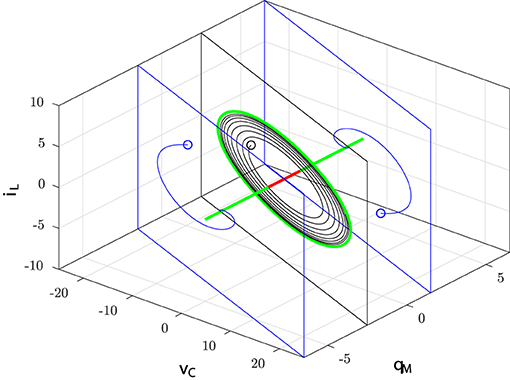
Figure 4. Stable (green half lines) and unstable (red segment) equilibrium points: the trajectories starting on the planes with and converge toward the corresponding equilibrium points; the trajectory starting on the plane with converges toward the stable limit cycle (green).
3.2. Limit Cycles
To investigate the presence of limit cycles on M(Q0) we resort to the DF method, a classical technique within the HB context. The DF method has been widely used for analyzing oscillatory behaviors in non-linear feedback control systems (see e.g., Gelb and Vander Velde, 1968; Atherton, 1975; Mees, 1981; Khalil, 2002). Within the HB setting, other techniques have been proposed to predict bifurcations of limit cycles and more complex dynamics (Genesio and Tesi, 1992; Piccardi, 1994; Tesi et al., 1996; Basso et al., 1997; Bonani and Gilli, 1999; Di Marco et al., 2003; Innocenti et al., 2010). The first step to apply the DF method is to show that system (7) admits the representation of Figure 5 whose dynamics is governed by the following input-output relation
where and are suitable rational functions.
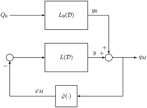
Figure 5. Equivalent input-output representation of system (7).
It is worth observing that this representation has an internal feedback interconnection between the linear subsystem and the non-linear subsystem described by the memristor characteristic, while is a feed-forward linear block driven by a constant input.
It can be readily verified that Equation (7) can be rewritten equivalently as a unique second order differential equation involving only qM. Since the second equation of Equation (7) becomes
Taking into account that , the above differential equation can be rearranged in the following equivalent input-output form
Hence, system (7) can be equivalently described via the input-output relation (10) with and given by
It is worth observing that is exactly the equivalent admittance of the linear part of the circuit with IS(t) = 0, i.e., the one seen at the terminals T′ and T′′ in Figure 1 where the memristor is connected.
The DF method looks for a first-order approximation of a periodic output qM(t) of the system of Figure 5, i.e.,
The corresponding periodic output φM(t) of period 2π/ω of the non-linear subsystem can be written as
where N0(A, B) is the bias gain and N1(A, B) is first harmonic gain, which are known as describing function terms, while φh(t) contains the higher order harmonics, i.e.,
with γh and θh, h = 2, …, being suitable constants.
The final step of the DF method consists in first computing the periodic signal of period 2π/ω given by the sum of the outputs y(t) and y0(t) of the two linear subsystems driven by −φM(t) and the constant signal Q0, respectively, then in equating the constant and the first order harmonic terms of the obtained periodic signal with the corresponding terms of qM(t), i.e., A and B. Taking into account that the constant and first order harmonic terms of φM(t) can be rewritten in an exponential form as and , respectively, the periodic signal given by the sum of y(t) and y0(t) can be computed by exploiting superposition and the expression of the response of a linear system which has the same exponential form of the input2. The so computed periodic signal has the following expression
where yh(t) contains the higher order harmonics generated by −φh(t). Then, by equating the constant term in Equation (17) with that of qM(t), we get the real equation
while by equating the first harmonic terms and taking into account that B cos ωt = B(ejωt + e−jωt)/2 we get the complex equation
In the HB approach, any first-order periodic signal (14) with A, B, and ω solving both Equations (18) and (19) is called a Predicted Limit Cycle (PLC) of the system of Figure 5. Also, it is expected that there exists a true limit cycle close to a PLC if the system of Figure 5 satisfies some conditions (see Atherton, 1975; Mees, 1981; Khalil, 2002 and references therein). These conditions basically rely on so-called filtering hypothesis which means that the non-linear subsystem does not generate large higher-order harmonics (i.e., φh(t) is small) and the two linear subsystems are low-pass filters (i.e., the gains |L(jhω)|, h = 2, …, are smaller than |L(0)| and |L(jω)|). Hence, this hypothesis requires that yh(t) must be much smaller than the constant and first order harmonic terms of Equation (17), according to some quantitative measure. For instance, in Di Marco et al. (2018) the distortion index is used to this purpose.
Now, to apply the DF method to the system under consideration, we observe that from Equation (13) we get L(0) = 0 and L0(0) = 1, while from Equations (1) and (15) it can be verified that the gains N0(A, B) and N1(A, B) have the following expressions:
Then, the Equation (18) reduces to
and the complex equation (19) boils down to
which can equivalently be written by separating the real and imaginary parts as
Equations (22), (24), and (25) are then solved for A = Â = Q0, and with such that
Hence, for each index Q0 such that there exists a PLC of the following form
This implies that each manifold M(Q0) contains a unique PLC for . Since
the trajectory described by the PLC in the (qM, iL)-plane lies on the following ellipse
Note that the ellipse is centered at the equilibrium point (Q0, 0) and its size is maximum at Q0 = 0 and decreases to zero as the index Q0 tends to , thus collapsing to the equilibrium point. Moreover, since for the equilibrium point is unstable and taking into account that the system is two dimensional, we can conclude that the PLC is stable. In this regard, we mention that PLC stability can be assessed also via approximate HB tools, such as the Loeb criterion (see e.g., Atherton, 1975; Tesi et al., 1996).
Summing up, we have shown that in the input-less memristor circuit there coexist infinitely many attractors: a stable equilibrium point for each value of the manifold index Q0 such that and a stable PLC for each value of the index Q0 such that . Figure 6 illustrates this multistability scenario for the following normalized values of the circuit parameters
from which it follows that .
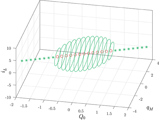
Figure 6. Input-less circuit attractors: stable (green ⋆) equilibrium points and stable PLCs (solid green) given by Equations (27) and (28) as a function of the manifold index Q0. The red circles denote the unstable equilibrium points.
In particular, it turns out that at a typical behavior of (supercritical) Hopf bifurcation is observed. However, since it is obtained by varying the index Q0 and thus the circuit initial conditions (for fixed circuit parameters), it may be referred to as a bifurcation without parameters (Corinto and Forti, 2017; Di Marco et al., 2018; Innocenti et al., 2019b; Ascoli et al., 2020a). As already discussed, it is expected that there exists a true limit cycle close to a PLC. Indeed, a more refined numerical analysis shows that for each |Q0| < 1 the corresponding invariant manifold M(Q0) has a unique limit cycle which attracts all the (non-trivial) trajectories. Moreover, the limit cycle is well-approximated by the PLC, as shown in Figure 7 for Q0 = 0.
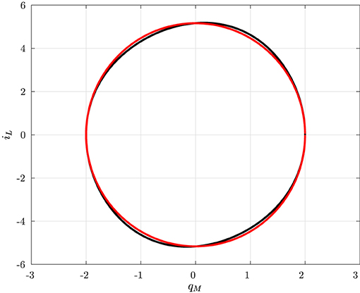
Figure 7. True limit cycle (solid dark) and PLC (solid red) in the (qM, iL)-plane for Q0 = 0.
A quantitative comparison between the PLCs and the true limit cycles is provided by Figure 8 where the maximum and the minimum of both the true periodic solution qM(t) and the PLC in Equation (27) are depicted as a function of the index Q0.
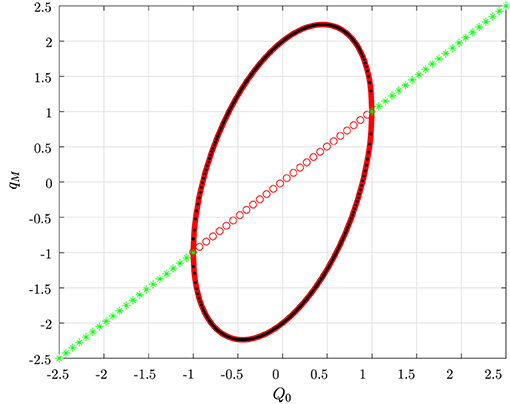
Figure 8. Stable (green ⋆) and unstable (red ◦) equilibrium points; maximum (32) and minimum (31) of the PLCs (solid red) as a function of Q0; maximum and minimum values of the numerically computed limit cycles (dotted dark points).
It can be readily checked that the minimum and the maximum of the first-order approximation are given by
and
respectively. We finally observe that similar results can be derived also for values of the circuit parameters different from those in Equation (30).
4. Modeling Neuron Dynamics via the Controlled Circuit
Section 3 makes it clear that in the input-less case the memristor circuit displays infinitely many attractors. Specifically, each planar invariant manifold M(Q0) contains either a unique stable equilibrium point or a stable limit cycle. Moreover, an approximation of the limit cycle belonging to M(Q0), with Q0 such that , is explicitly obtained in terms of the PLC (27).
In this section it will be shown how the coexistence of infinitely many stable equilibrium points and limit cycles, together with the knowledge of their dependence on the manifold index Q0, which in the case of limit cycles is given in an approximate way by Equation (27), can be suitably exploited to make the memristor charge qM responding as in Figure 2B to a pulse shaped input source Is. To proceed, we consider the circuit state equations (3) by replacing vC with the following state variable
It turns out that (3) reduces to the third-order system
where Q, qM, and iL are the new state variables. Suppose that at time t = ti ≥ t0 the current source Is(t) displays a pulse of area Λ and width Δ > 0, i.e., Is(t) is equal to zero for t ∈ [t0, ti] and t ∈ [ti + Δ, +∞) and such that
From the first equation of Equation (34) it follows that
which implies for t ∈ [t0, ti] and for t ∈ [ti + Δ, +∞). For instance, in the case of a rectangular pulse we have .
By comparing the second and third equations of Equation (34) with those of Equation (7), it follows that the circuit dynamics lies onto for t ∈ [t0, ti], it moves toward during the interval [ti, ti + Δ], it reaches at t = ti + Δ, where it remains for all t ≥ ti + Δ. Hence, the circuit has the property that pulse shaped current sources Is make the dynamics moving from an initial manifold to any other one within a given time interval, by suitably choosing the pulse area and width.
We are interested in the case where the manifold has a stable equilibrium point and in particular the index is negative and hence . Moreover, we assume that at t = ti the circuit state is at the equilibrium point, which means that . Let us now investigate the dynamics induced by a rectangular pulse of positive area Λ and width Δ on the circuit dynamics. It turns out that the final manifold still contains a stable equilibrium point if , while it contains a stable limit cycle if and again a stable equilibrium point if . Figure 9 illustrates the first two possible behaviors in the case of a rectangular pulse of height A/Δ with the circuit parameters as in (30).
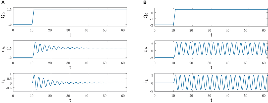
Figure 9. Dynamics generated by applying at ti = 10 a rectangular pulse of area Λ and width Δ = 1 via the current source Is; the circuit parameters are as in Equation (30) and the initial conditions are qM(0) = −2 and IL(0) = 0, while Q(0) = −2. (A) For Λ = 0.5, the index Q(t) and the state variables qM(t), iL(t) converge to Q0 = −1.5 and to the equilibrium point (−1.5, 0), respectively. (B) For Λ = 2.5, Q(t) converges to Q0 = 0.5 and the state variables qM(t), iL(t) converge to the limit cycle belonging to the manifold M(0.5).
Specifically, after reaching at time t = ti + Δ at the point (Q(ti + Δ), qM(ti + Δ), iL(ti + Δ)) with , the dynamics converges toward the attractor contained in the manifold, an equilibrium point in Figure 9A and a limit cycle in Figure 9B.
Clearly, the length of the transient behavior toward the attractor depends on the values of qM(ti + Δ) and iL(ti + Δ). The farther away is the point (qM(ti + Δ), iL(ti + Δ)) from the attractor lying onto , the longer is the transient. Clearly, if (qM(ti + Δ), iL(ti + Δ)) belongs to the attractor we have no transient behavior. The values of qM(ti + Δ) and iL(ti + Δ) cannot be computed explicitly since this would require to integrate the second and third equations of (34) in the interval [ti, ti + Δ] with the initial condition and . However, by employing a Taylor series expansion for qM(t) and iL(t) for t ∈ [ti, ti + Δ], it turns out that
where αi and βi, i = 1, 2 are constants. It is interesting to note that if the width Δ of the pulse is small, then for t ∈ [ti, ti + Δ] the charge qM remains almost constant, while iL varies from zero to a quantity proportional to Δ.
Summing up, for a suitable choice of the pulse area A and for sufficiently small width Δ, the pulse current Is is able to steer, within the interval [ti, ti + Δ], the dynamics from the stable equilibrium point of to the manifold containing a stable limit cycle. Moreover, during the time interval the charge qM is almost constant and the current iL remains close to zero.
We are now ready to show how it is possible to make the charge qM display a behavior similar to that of Figure 2B in response to a pulse shaped input source Is. Here, we are more interested in the dynamic response of the neuron than in its set and reset mechanisms. For these mechanisms we simply adopt the pulse timing of Figure 10 which is assumed to be generated via suitable logic gates.
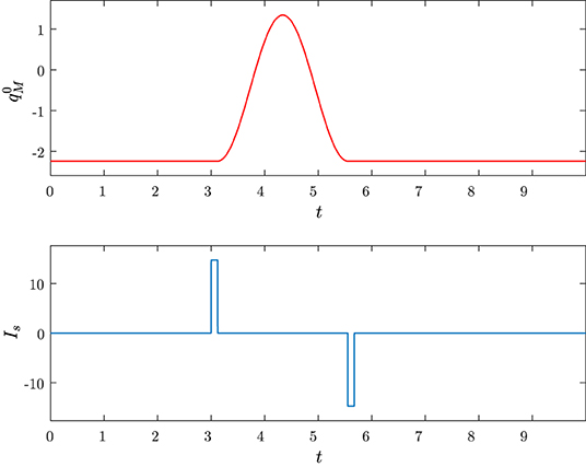
Figure 10. Top: predicted behavior of the memristor charge. Bottom: timing of the current pulses.
At time t = ti the hardware detects a stimulus and generates a current pulse Is with area A and width Δ (set mechanism), which moves the dynamics away from the stable equilibrium point (resting point) in ; at time t = ti + Δ the dynamics reaches and the memristor charge qM starts displaying a behavior similar to that reported in Figure 2B; at time t = ti + Δ + T an inverse current pulse is generated in order to make the dynamics come back to the stable equilibrium point in (reset mechanism).
Hence, the problem is how the parameters , Λ, Δ, and T should be designed in order to obtain the sought behavior of qM. Let Δ be chosen enough small to ensure, as discussed above, that in [ti, ti + Δ] the charge qM is almost constant and the current iL remains close to zero. Choosing a small Δ implies that when at t = ti + Δ the dynamics reaches the manifold we have that qM and iL are quite close to and zero, respectively. This manifold contains a stable limit cycle which can be in general computed only numerically. However, in section 3 it has been shown that the limit cycle can be approximated by a PLC. Clearly, the current expression of the PLC on is obtained by putting in Equation (27).
Now, observe that the minimum and the maximum values of qM, expressed in Equations (31) and (32), respectively, are achieved once iL is equal to zero. Hence, since for sufficiently small Δ we have that , it is possible to set (qM(ti + Δ), iL(ti + Δ)) as the point of the manifold where the PLC has its minimum value (31). Consequently, for t ∈ [ti + Δ, ti + Δ + T] with T being the PLC period, the PLC provides the typical harmonic oscillator over one period, i.e., it evolves from the minimum to the maximum coming back again to the minimum. At the end of the period, the reset mechanism generates a current pulse of area −A and width Δ, which makes the dynamics come back to the stable equilibrium point of . Hence, the resulting behavior of the memristor charge can be expressed as
and is depicted in Figure 10. Note that the parameter T has been chosen as the period of the PLC, i.e.:
Hereafter, we denote by the time-derivative of , i.e.:
Now, to set (qM(ti + Δ), iL(ti+Δ)) as the point of the manifold where the PLC has its minimum value (31), the following condition must be satisfied
with . It is not difficult to verify that there are many solutions and Q0 of (41) such that and . We are interested in the one with the minimum value of because this choice ensures that the stable equilibrium point on the initial manifold is at the maximum distance from the invariant manifold where the Hopf bifurcation happens, thus guaranteeing a larger robustness margin against spurious pulses of small area. The minimum value of can be computed in closed form by minimizing the right hand side of Equation (41). It turns out that
and since
from Equations (41) and (9) we have
Moreover, since Q0 in Equation (41) stands for , from Equation (42) we finally get
Finally, the pulse width Δ should be practically chosen to be some percent of the period T. Hence, we can select it according to the relation
where σ lies in the interval [0.01, 0.05].
Summing up, to obtain in Equation (38), the parameters T, , Λ, and Δ can be designed according to the corresponding expressions given in Equations (39), (43), (44), and (45), respectively. Notably, these relations depend explicitly on the circuit parameters R, L, C, s0, and s1. Hence, by suitably adapting these parameters it is possible to vary the features of .
On the other hand, the formulas in Equations (39), (43), (44), and (45) have been derived under two approximations. The first one concerns the assumption that at time t = ti + Δ the values of qM and iL are quite close to and zero, respectively. However, according to Equation (37) by lowering the value of the pulse width this assumption can be suitably satisfied. The second approximation is that the formulas have been obtained by using the PLCs instead of the true limit cycles. Indeed, as shown in section 3.2, the true limit cycles contain higher order harmonics terms which can generate some distortion in both the period and the minimum and maximum amplitudes over the period, with respect to those analytically computed for the PLCs. However, these higher order harmonics can be filtered out by suitably adjusting the circuit parameters. Moreover, the fact that the input-less memristor circuit contains a bundle of limit cycles makes the formulas, and hence the parameter design procedure, sufficiently robust with respect to the use of PLC in their derivation. Said another way, by slightly varying the parameters T, , A, and Δ from the nominal values provided by Equations (39), (43), (44), and (45), respectively, the distortion effect could be reduced.
To illustrate the design procedure let us consider the circuit parameters in Equation (30). From Equations (39), (43), and (44), we have that
and choosing σ = 0.02 in Equation (45) we obtain
The corresponding predicted behavior in Equation (38) is reported Figure 11A together with the true behavior of qM(t) which is obtained by solving numerically (34). The state space trajectories corresponding to the true solution (Q(t), qM(t), iL(t)) of the circuit and the predicted solution ) are depicted in Figure 11B.
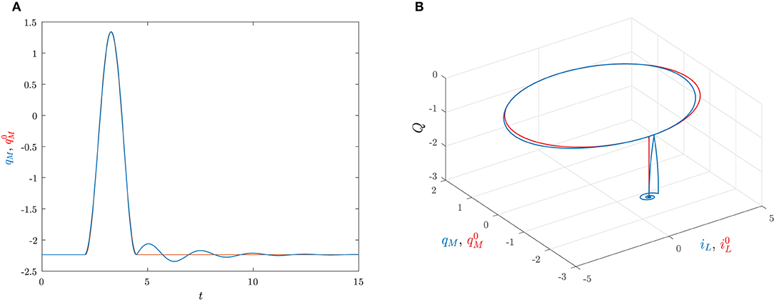
Figure 11. The set pulse is applied at ti = 2 with area A = 1.7889 and width Δ = 0.0487, the reset pulse is applied at ti + Δ + T = 4.4821 with area Λ = −1.7889 and width Δ = 0.0487. The initial conditions are Q(0) = −2.2361, qM(0) = −2.2361 and iL(0) = 0. (A) Time behaviors of qM (blu) and (red). (B) Trajectories in the state space generated by (Q(t), qM(t), iL(t)) (blu) and (red).
Note that the charge qM(t) has a dynamical behavior that is quite similar to the one depicted in Figure 2B, thus clearly showing that the memristor circuit can be used for mimicking some features of neuron dynamics.
This dynamical similarity is confirmed also in other scenarios. For instance, suppose that in the pulse timing the reset pulse is activated at t = ti + Δ + nT, with n being a positive integer. Clearly, in this case completes n periods within the interval ti + Δ, ti + Δ + nT, and, therefore, qM(t) is expected to generate a burst of n spikes. Figure 12 provides the numerically computed behavior of qM(t) for n = 8 over a time frame covering three bursts.
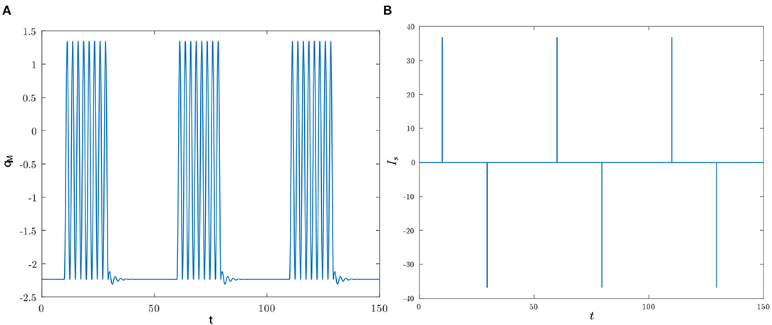
Figure 12. The initial conditions are as in Figure 11, the set pulses are activated at ti ∈ {10, 60, 110} and the reset pulses are applied 19.5164 time units later. (A) Time behavior of qM for n = 8. (B) Time behavior of Is.
5. Conclusions
In this paper, a memristor circuit composed of a resistor, an inductor, a capacitor, an ideal charge-controlled memristor and an independent current source as input is considered. It is first shown that in the input-less case the circuit enjoys the foliation property of the state space, i.e., it contains infinitely many planar invariant manifolds which are parameterized by a scalar index depending on the circuit initial conditions. Each manifold contains an attractor which can be either a stable equilibrium point or a stable limit cycle, depending on the value of the manifold index. Moreover, a first-order periodic approximation is obtained in an analytic way for each limit cycle via the Describing Function (DF) technique, a classical tool within the Harmonic Balance (HB) context.
Then, it is shown that the memristor charge can mimic a simplified model of a neuron response when an external independent pulse-programmed current source is introduced in the circuit. Specifically, the sought dynamics of the memristor charge is generated via the concatenation of convergent and oscillatory behaviors, which are obtained by switching between stable equilibrium points and limit cycles via a suitable design of the pulse timing of the current source. Some relationships between the pulse and the circuit parameters are also devised exploiting the knowledge of the first-order periodic approximation of the limit cycles.
Data Availability Statement
The raw data supporting the conclusions of this article will be made available, without undue reservation, on request to the corresponding author with appropriate motivation.
Author Contributions
All authors contributed to the conception and design of the study, wrote the manuscript, read, and approved the submitted version.
Funding
This work was supported by the project Analogue COmputing with Dynamic Switching Memristor Oscillators: Theory, Devices and Applications (COSMO), Grant PRIN 2017LSCR4K 002, funded by the Italian Ministry of Education, University and Research (MIUR).
Conflict of Interest
The authors declare that the research was conducted in the absence of any commercial or financial relationships that could be construed as a potential conflict of interest.
Footnotes
1. ^Throughout the paper, denotes the derivative of the function f(t) at .
2. ^Consider a linear time-invariant finite-dimensional causal system described by the input-output relation where the operator has the following general form
with ai, bi, i = 0, …, n − 1 being constants. Let u(t) be an exponential signal, i.e., u(t) = Ceσt, C ∈ ℝ, σ ∈ ℂ, and assume that L(σ) is finite, i.e., L(σ) ≠ ∞. Then, for suitable initial conditions of the system, we have y(t) = CL(σ)eσt, i.e., the output of the system has the same exponential form of the input.
References
Adhikari, S. P., Yang, C., Kim, H., and Chua, L. O. (2012). Memristor bridge synapse-based neural network and its learning. IEEE Trans. Neural Netw. Learn. Syst. 23, 1426–1435. doi: 10.1109/TNNLS.2012.2204770
Ascoli, A., Messaris, I., Tetzlaff, R., and Chua, L. O. (2020a). Theoretical foundations of memristor cellular nonlinear networks: stability analysis with dynamic memristors. IEEE Trans. Circ. Syst. I Reg. Pap. 67, 1389–1401. doi: 10.1109/TCSI.2019.2957813
Ascoli, A., Tetzlaff, R., Kang, S. M., and Chua, L. O. (2020b). Theoretical foundations of memristor cellular nonlinear networks: A DRM2-based method to design memcomputers with dynamic memristors. IEEE Trans. Circ. Syst. I Reg. Pap. 67, 2753–2766. doi: 10.1109/TCSI.2020.2978460
Babacan, Y., Kaçar, F., and Gürkan, K. (2016). A spiking and bursting neuron circuit based on memristor. Neurocomputing 203, 86–91. doi: 10.1016/j.neucom.2016.03.060
Basso, M., Genesio, R., and Tesi, A. (1997). A frequency method for predicting limit cycle bifurcations. Nonlinear Dyn. 13, 339–360. doi: 10.1023/A:1008298205786
Bonani, F., and Gilli, M. (1999). Analysis of stability and bifurcations of limit cycles in Chua's circuit through the harmonic-balance approach. IEEE Trans. Circ. Syst. I Fundament. Theory Appl. 46, 881–890. doi: 10.1109/81.780370
Bonomi, F., Milito, R., Zhu, J., and Addepalli, S. (2012). “Fog computing and its role in the internet of things,” in Proceedings of the First Edition of the MCC Workshop on Mobile Cloud Computing (Helsinki: ACM), 13–16. doi: 10.1145/2342509.2342513
Chen, M., Sun, M., Bao, B., Wu, H., Xu, Q., and Wang, J. (2018). Controlling extreme multistability of memristor emulator-based dynamical circuit in flux-charge domain. Nonlinear Dyn. 91, 1395–1412. doi: 10.1007/s11071-017-3952-9
Chen, Z., Zheng, M., Friesen, W. O., and Iwasaki, T. (2008). Multivariable harmonic balance analysis of the neuronal oscillator for leech swimming. J. Comput. Neurosci. 25:583. doi: 10.1007/s10827-008-0105-7
Chua, L., Sbitnev, V., and Kim, H. (2012). Hodgkin-Huxley axon is made of memristors. Int. J. Bifurc. Chaos 22:1230011. doi: 10.1142/S021812741230011X
Chua, L. O. (1971). Memristor-the missing circuit element. IEEE Trans. Circ. Theory 18, 507–519. doi: 10.1109/TCT.1971.1083337
Corinto, F., Ascoli, A., and Gilli, M. (2011). Nonlinear dynamics of memristor oscillators. IEEE Trans. Circ. Syst. I Reg. Pap. 58, 1323–1336. doi: 10.1109/TCSI.2010.2097731
Corinto, F., Di Marco, M., Forti, M., and Chua, L. (2019). Nonlinear networks with mem-elements: complex dynamics via flux-charge analysis method. IEEE Trans. Cybern. 1–14. doi: 10.1109/TCYB.2019.2904903
Corinto, F., and Forti, M. (2016). Memristor circuits: flux-charge analysis method. IEEE Trans. Circ. Syst. I Reg. Pap. 63, 1997–2009. doi: 10.1109/TCSI.2016.2590948
Corinto, F., and Forti, M. (2017). Memristor circuits: bifurcations without parameters. IEEE Trans. Circ. Syst. I Reg. Pap. 64, 1540–1551. doi: 10.1109/TCSI.2016.2642112
Corinto, F., and Forti, M. (2018). Memristor circuits: pulse programming via invariant manifolds. IEEE Trans. Circ. Syst. I Reg. Pap. 65, 1327–1339. doi: 10.1109/TCSI.2017.2740999
Di Marco, M., Forti, M., Innocenti, G., and Tesi, A. (2018). Harmonic balance method to analyze bifurcations in memristor oscillatory circuits. Int. J. Circ. Theory Appl. 46, 66–83. doi: 10.1002/cta.2414
Di Marco, M., Forti, M., Innocenti, G., and Tesi, A. (2020a). “Input design for controlling dynamics in a second-order memristive circuit,” in 2020 European Conference on Circuit Theory and Design (ECCTD) (Sofia), 1–4. doi: 10.1109/ECCTD49232.2020.9218368
Di Marco, M., Forti, M., Innocenti, G., and Tesi, A. (2021). “Transient control in targeting multistable dynamics of a memristor circuit,” in 2021 IEEE International Symposium on Circuits and Systems (ISCAS 2021) (Daegu: IEEE). doi: 10.1109/ISCAS51556.2021.9401351
Di Marco, M., Forti, M., Innocenti, G., Tesi, A., and Corinto, F. (2020b). “Targeting multistable dynamics in a second-order memristor circuit,” in 2020 IEEE International Symposium on Circuits and Systems (ISCAS) (Seville), 1–5. doi: 10.1109/ISCAS45731.2020.9181111
Di Marco, M., Forti, M., and Pancioni, L. (2016). Complete stability of feedback CNNs with dynamic memristors and second-order cells. Int. J. Circ. Theory Appl. 44, 1959–1981. doi: 10.1002/cta.2205
Di Marco, M., Forti, M., and Pancioni, L. (2017). Convergence and multistability of nonsymmetric cellular neural networks with memristors. IEEE Trans. Cybern. 47, 2970–2983. doi: 10.1109/TCYB.2016.2586115
Di Marco, M., Forti, M., and Pancioni, L. (2017). Memristor standard cellular neural networks computing in the flux-charge domain. Neural Netw. 93, 152–164. doi: 10.1016/j.neunet.2017.05.009
Di Marco, M., Forti, M., and Tesi, A. (2003). Harmonic balance approach to predict period-doubling bifurcations in nearly-symmetric neural networks. J. Circ. Syst. Comput. 12, 435–460. doi: 10.1142/S0218126603000969
Di Marco, M., Innocenti, G., Forti, M., and Tesi, A. (2019). “Control design for targeting dynamics of memristor Murali-Lakshmanan-Chua circuit,” in IEEE ECC 2019 (Naples), 4332–4337. doi: 10.23919/ECC.2019.8795813
Du, C., Cai, F., Zidan, M. A., Ma, W., Lee, S. H., and Lu, W. D. (2017). Reservoir computing using dynamic memristors for temporal information processing. Nat. Comm. 8:2204. doi: 10.1038/s41467-017-02337-y
Gelb, A., and Vander Velde, W. E. (1968). Multiple-Input Describing Functions and Nonlinear System Design. New York, NY: McGraw-Hill Book Co.
Genesio, R., and Tesi, A. (1992). Harmonic balance methods for the analysis of chaotic dynamics in nonlinear systems. Automatica 28, 531–548. doi: 10.1016/0005-1098(92)90177-H
Hong, Q., Zhao, L., and Wang, X. (2019). Novel circuit designs of memristor synapse and neuron. Neurocomputing 330, 11–16. doi: 10.1016/j.neucom.2018.11.043
Hu, M., Chen, Y., Yang, J. J., Wang, Y., and Li, H. H. (2016). A compact memristor-based dynamic synapse for spiking neural networks. IEEE Trans. Comput. Aided Design Integr. Circ. Syst. 36, 1353–1366. doi: 10.1109/TCAD.2016.2618866
Ielmini, D., and Pedretti, G. (2020). Device and circuit architectures for in-memory computing. Adv. Intell. Syst. 2:2000040. doi: 10.1002/aisy.202000040
Ielmini, D., and Wong, H.-S. P. (2018). In-memory computing with resistive switching devices. Nat. Electron. 1:333. doi: 10.1038/s41928-018-0092-2
Innocenti, G., Di Marco, M., Forti, M., and Tesi, A. (2019a). “A controlled Murali-Lakshmanan-Chua memristor circuit to mimic neuron dynamics,” in 2019 IEEE 58th Conference on Decision and Control (CDC) (Nice: IEEE), 3423–3428. doi: 10.1109/CDC40024.2019.9029330
Innocenti, G., Di Marco, M., Forti, M., and Tesi, A. (2019b). Prediction of period doubling bifurcations in harmonically forced memristor circuits. Nonlinear Dyn. 96, 1169–1190. doi: 10.1007/s11071-019-04847-4
Innocenti, G., Di Marco, M., Tesi, A., and Forti, M. (2020). Input-output characterization of the dynamical properties of circuits with a memelement. Int. J. Bifurc. Chaos 30:2050110. doi: 10.1142/S0218127420501102
Innocenti, G., Tesi, A., and Genesio, R. (2010). Complex behaviour analysis in quadratic jerk systems via frequency domain Hopf bifurcation. Int. J. Bifurc. Chaos 20, 657–667. doi: 10.1142/S0218127410025946
Izhikevich, E. M. (2000). Neural excitability, spiking and bursting. Int. J. Bifurc. Chaos 10, 1171–1266. doi: 10.1142/S0218127400000840
Izhikevich, E. M. (2007). Dynamical Systems in Neuroscience. Cambridge, MA: MIT Press. doi: 10.7551/mitpress/2526.001.0001
Jo, S. H., Chang, T., Ebong, I., Bhadviya, B. B., Mazumder, P., and Lu, W. (2010). Nanoscale memristor device as synapse in neuromorphic systems. Nano Lett. 10, 1297–1301. doi: 10.1021/nl904092h
Kim, S., Du, C., Sheridan, P., Ma, W., Choi, S., and Lu, W. D. (2015). Experimental demonstration of a second-order memristor and its ability to biorealistically implement synaptic plasticity. Nano Lett. 15, 2203–2211. doi: 10.1021/acs.nanolett.5b00697
Krestinskaya, O., James, A. P., and Chua, L. O. (2020). Neuromemristive circuits for edge computing: a review. IEEE Trans. Neural Netw. Learn. Syst. 31, 4–23. doi: 10.1109/TNNLS.2019.2899262
Kumar, S., Strachan, J. P., and Williams, R. S. (2017). Chaotic dynamics in nanoscale NbO2 Mott memristors for analogue computing. Nature 548:318. doi: 10.1038/nature23307
Matsuoka, K. (2011). Analysis of a neural oscillator. Biol. Cybernet. 104, 297–304. doi: 10.1007/s00422-011-0432-z
Nakada, K. (2019). An ReRAM-based neuron device for neuromorphic pulse coding. Jpn. J. Appl. Phys. 58:030904. doi: 10.7567/1347-4065/aafb60
Pershin, Y. V., and Di Ventra, M. (2011). Memory effects in complex materials and nanoscale systems. Adv. Phys. 60, 145–227. doi: 10.1080/00018732.2010.544961
Piccardi, C. (1994). Bifurcations of limit cycles in periodically forced nonlinear systems: the harmonic balance approach. IEEE Trans. Circ. Syst. I 41, 315–320. doi: 10.1109/81.285687
Pisarchik, A. N., and Feudel, U. (2014). Control of multistability. Phys. Rep. 540, 167–218. doi: 10.1016/j.physrep.2014.02.007
Satyanarayanan, M. (2017). The emergence of edge computing. Computer 50, 30–39. doi: 10.1109/MC.2017.9
Tesi, A., Abed, E. H., Genesio, R., and Wang, H. O. (1996). Harmonic balance analysis of period-doubling bifurcations with implications for control of nonlinear dynamics. Automatica 32, 1255–1271. doi: 10.1016/0005-1098(96)00065-9
Thomas, A. (2013). Memristor-based neural networks. J. Phys. D Appl. Phys. 46:093001. doi: 10.1088/0022-3727/46/9/093001
Usha, K., and Subha, P. (2019). Hindmarsh-Rose neuron model with memristors. Biosystems 178, 1–9. doi: 10.1016/j.biosystems.2019.01.005
Wang, N., Zhang, G., and Bao, H. (2019). Bursting oscillations and coexisting attractors in a simple memristor-capacitor-based chaotic circuit. Nonlinear Dyn. 97, 1477–1494. doi: 10.1007/s11071-019-05067-6
Wang, Z., Ambrogio, S., Balatti, S., and Ielmini, D. (2015). A 2-transistor/1-resistor artificial synapse capable of communication and stochastic learning in neuromorphic systems. Front. Neurosci. 8:438. doi: 10.3389/fnins.2014.00438
Williams, R. S. (2017). What's next? [The end of Moore's law]. Comput. Sci. Eng. 19, 7–13. doi: 10.1109/MCSE.2017.31
Xu, Q., Lin, Y., Bao, B., and Chen, M. (2016). Multiple attractors in a non-ideal active voltage-controlled memristor based Chua's circuit. Chaos Solitons Fractals 83, 186–200. doi: 10.1016/j.chaos.2015.12.007
Yang, J. J., Strukov, D. B., and Stewart, D. R. (2013). Memristive devices for computing. Nat. Nanotechnol. 8, 13–24. doi: 10.1038/nnano.2012.240
Yuan, F., Wang, G., Jin, P., Wang, X., and Ma, G. (2016). Chaos in a meminductor-based circuit. Int. J. Bifurc. Chaos 26:1650130. doi: 10.1142/S0218127416501303
Keywords: neuron, spiking, bursting, memristor, pulse-programmed circuit, harmonic balance
Citation: Innocenti G, Di Marco M, Tesi A and Forti M (2021) Memristor Circuits for Simulating Neuron Spiking and Burst Phenomena. Front. Neurosci. 15:681035. doi: 10.3389/fnins.2021.681035
Received: 15 March 2021; Accepted: 10 May 2021;
Published: 10 June 2021.
Edited by:
Kyeong-Sik Min, Kookmin University, South KoreaReviewed by:
Kazuki Nakada, Hiroshima City University, JapanAlon Ascoli, Technische Universität Dresden, Germany
Copyright © 2021 Innocenti, Di Marco, Tesi and Forti. This is an open-access article distributed under the terms of the Creative Commons Attribution License (CC BY). The use, distribution or reproduction in other forums is permitted, provided the original author(s) and the copyright owner(s) are credited and that the original publication in this journal is cited, in accordance with accepted academic practice. No use, distribution or reproduction is permitted which does not comply with these terms.
*Correspondence: Giacomo Innocenti, giacomo.innocenti@unifi.it