 Gilsoon Park
 Kichang Kwak
 Sang Won Seo
 Jong-Min Lee
- 1Department of Biomedical Engineering, Hanyang University, Seoul, South Korea
- 2McGill Centre for Integrative Neuroscience, Montreal Neurological Institute, McGill University, Montreal, QC, Canada
- 3Department of Neurology, Samsung Medical Center, Sungkyunkwan University School of Medicine, Seoul, South Korea
In this paper, we introduce a novel automatic method for Corpus Callosum (CC) in midsagittal plane segmentation. The robust segmentation of CC in midsagittal plane is key role for quantitative study of structural features of CC associated with various neurological disorder such as epilepsy, autism, Alzheimer's disease, and so on. Our approach is based on Bayesian inference using sparse representation and multi-atlas voting which both methods are used in various medical imaging, and show outstanding performance. Prior information in the proposed Bayesian inference is obtained from probability map generated from multi-atlas voting. The probability map contains the information of shape and location of CC of target image. Likelihood in the proposed Bayesian inference is obtained from gamma distribution function, generated from reconstruction errors (or sparse representation error), which are calculated in sparse representation of target patch using foreground dictionary and background dictionary each. Unlike the usual sparse representation method, we added gradient magnitude and gradient direction information to the patches of dictionaries and target, which had better segmentation performance than when not added. We compared three main segmentation results as follow: (1) the joint label fusion (JLF) method which is state-of-art method in multi-atlas voting based segmentation for evaluation of our method; (2) prior information estimated from multi-atlas voting only; (3) likelihood estimated from comparison of the reconstruction errors from sparse representation error only; (4) the proposed Bayesian inference. The methods were evaluated using two data sets of T1-weighted images, which one data set consists of 100 normal young subjects and the other data set consist of 25 normal old subjects and 22 old subjects with heavy drinker. In both data sets, the proposed Bayesian inference method has significantly the best segmentation performance than using each method separately.
Introduction
The Corpus Callosum (CC), the largest white matter (WM) structure placed beneath the cortex of the human brain, connects homologous cortical areas of the two cerebral hemispheres (Caminiti et al., 2009). It has been shown that many neurological diseases give rise to changes of structural feature of the CC such as size and shape, for example epilepsy (O'Dwyer et al., 2010; Firat et al., 2014), autism (Frazier et al., 2012; Prigge et al., 2013), schizophrenia (Kim et al., 2012; Joshi et al., 2013; Balevich et al., 2015), dyslexia (Casanova et al., 2010; Elnakib et al., 2012), Alzheimer's disease (Zhu et al., 2014; Elahi et al., 2015; Wang et al., 2015) and in the effect of heavy drinking (Bookstein et al., 2002), and smoking (Lin et al., 2013). The CC defined in midsagittal plane (MSP) of the magnetic resonance imaging (MRI) has been generally used because it has relatively clear boundary line and mirrors overall properties of CC (Casanova et al., 2010; O'Dwyer et al., 2010; Joshi et al., 2013; Firat et al., 2014; Zhu et al., 2014; Balevich et al., 2015; Elahi et al., 2015; Wang et al., 2015). Accurate segmentation of CC in MSP is important for the quantitative and qualitative studies of the neurological diseases related to CC.
The manual segmentation of CC is a laborious and time-consuming task. It also has inter-intra variability problem. The more data there is, the more these problems become more serious. For solving the problems resulting from manual segmentation, Various automated methods have been proposed to segment CC (He et al., 2007; Shyu et al., 2012; Içer, 2013; Yeo et al., 2014). Although the general shape of the CC is relatively regular, automated segmentation of CC has been still challenging because the detail shape is dynamic and the fornix, bundle of never fibers located around CC, has exceedingly similar intensity as CC.
Voxel intensity-based segmentation is one of the most popular approaches. Semra Içer proposed the estimated Gaussian mixture model and fuzzy C means from intensity distribution of CC (Içer, 2013). Voxel intensity-based segmentation, however, cannot work well if data has noise or the structures like target structure because it did not consider local information, intensity information of neighborhood voxels in a target voxel. Active Contour Model (ACM) is also popularly used to segment CC. For segmentation of target structure, ACM uses energy consisting of external and internal force. The external force is image features such as gradients and lines and the internal force is the relationship between points of contour. Both the external and internal force develop initial contour to boundary of target structure. He et al. proposed a context-sensitive active contour based on evolving four seed contours, forming interconnected parts made by initial points, into CC boundary line according to each motion law (He et al., 2007). Shyu et al. introduced an ACM based on region-based local intensity with a global density distance (Shyu et al., 2012). Yeo et al. introduced a level-set model based on Bayesian inference, which drew the active contour to the target structure according to image feature and shape prior (Yeo et al., 2014). Although ACM has more robust segmentation performance than the voxel intensity-based segmentation because of considering various information around contour, ACM-based segmentation cannot work well if the initial contour is set far from target structure. Furthermore, it is difficult to segment detailed part of target structure having severe variation because of internal energy.
Recently, the multi-atlas voting method and the patch-based method have been widely used in medical imaging and show good performance in practice (Liu et al., 2012; Tong et al., 2013; Asman et al., 2015; Kim et al., 2015; Sanroma et al., 2015; Zhang et al., 2015; Doshi et al., 2016). The multi-atlas voting method developed from single-atlas -based segmentation. Single-atlas based segmentation estimates a target structure of an unseen image using an atlas image we know the right answer of the target structure (Andreasen et al., 1996; Cuadra et al., 2004). When applied to the target image with heavily variation, the single atlas based segmentation generally shows poor performance due to registration error. Multi-atlas voting based segmentation, which uses multiple atlases instead of just one atlas, has been proposed to overcome this issue. For final segmentation result in multi-atlas voting based segmentation, multi-classifier voting algorithm such as majority voting and STAPLE is required (Warfield et al., 2004). Aljabar et al. suggested atlas selection, where subset atlas appropriate for target image are selected through similarity index between atlas and target image in order to reduce registration error and computational time (Aljabar et al., 2009). The multi-atlas voting based segmentation is still vulnerable to the detailed estimation of the brain structure when the number of atlas is limited and variation of the target image is large. Patch-based segmentation uses abundant neighborhood features (e.g., intensity or gradient) of a target voxel in target image, overcoming lake of local information. Sparse representation, a patch-based technique, has been introduced in various image processing fields such as denosing (Elad and Aharon, 2006), restoration (Mairal et al., 2008), and face recognition (Wright et al., 2009; Yang and Zhang, 2010). The basic concept of sparse representation is that an input target image could be reconstructed as a sparse linear combination of dictionary samples consisting of training images via L1-norm minimization (Donoho, 2006). Sparse representation procedure results in generating sparse coefficients and reconstruction error between the target image and the sparse approximate image (Donoho, 2006). Recently, sparse representation technique has been applied successfully in neuroimaging fields such as volume registration (Kim et al., 2015), hippocampus segmentation (Tong et al., 2013), AD classification (Liu et al., 2012), and brain parcellation (Zhang et al., 2015). Since the segmentation method using sparse representation is based on abundant local information, it has good performance about the detailed part of target structure. But it is ineffective about overall shape in comparison with multi-atlas voting. In this paper, we combined the strengths of multi-atlas voting method and sparse representation method for CC segmentation. The proposed method avoids the disadvantages of the pervious CC segmentation methods and has better performance than multi-atlas voting method and sparse representation method, respectively.
There have been several studies in which the target structure is segmented by combining two type information. Patenaude et al. built a Bayesian framework, consisting of probabilistic relationships between shape and intensity extracted atlas images, to segment subcortical region of target image (Patenaude et al., 2011). Sanroma et al. introduced a novel segmentation method that fused two types of patch-based label fusion approaches, reconstruction-based approaches and classification-based approaches, using matrix completion for segmentation of various brain structures (Sanroma et al., 2015). These methods prove that segmentation method with a good combination of the two types of information can lead to better performance than single type information.
We combined information extracted from sparse representation and multi-atlas voting using Bayesian inference framework. Bayesian inference has been used in various fields for a long time. It effectively combines prior information and likelihood. Prior information can be specified by the user, but usually represents a natural probability. In other words, it calculates the probability that the target belongs to each class based on the experience so far. In this paper, it is extracted from the probability map resulting from multi-atlas voting. Since likelihood is calculated based on certain condition, we estimate the class-conditional probability that agrees with the distribution of reconstruction errors generated from sparse representation in each class. Multi-atlas voting based segmentation has good segmentation performance toward global information such as overall shape and location since atlases effectively catch the global information of the target image using registration. Patch-based segmentation (i.e., sparse representation based segmentation) well catches local information such as detailed shape variation since patches contain relation between target voxel and its neighborhood voxels. We could successfully mix the two types of information, which are global and local generated from multi-atlas voting and sparse representation respectively, in Bayesian inference. To the best of our knowledge, a combined method of sparse representation and multi-atlas voting in Bayesian inference has not been used for segmentation.
In this paper, we proposed a novel Bayesian inference consisting of sparse representation and multi-atlas voting for CC segmentation. The proposed method used the sparse representation error of target image as the likelihood and the probability map of CC generated from multi-atlas voting as a prior information. We compared the performance of the proposed method with those of other related methods as follow: (1) the joint label fusion (JLF) method which is state-of-art method in multi-atlas voting based segmentation for evaluation of our method; (2) prior information estimated from multi-atlas voting only; (3) likelihood estimated from sparse representation error (LESRE) only; (4) the proposed Bayesian inference consisting of sparse representation error as likelihood and probability map of CC as a prior. Finally, we validated robustness and accuracy by applying the proposed method to the two data set, where one consists of young healthy group and the other consists of heavy drinkers that generally have large variability of CC shape (Bookstein et al., 2002).
Methods
Data Acquisition
We used two different data sets for evaluation (Table 1). The first data set (“OASIS”) was selected from Open Access Series of Imaging Studies (OASIS) database (www.oasis-brain.org), which consists of three or four individual T1-weighted MR brain images of 416 subjects. We randomly selected 100 normal male and female subjects among them (50 males, age range = 18–28 years, mean age = 22.1 years, standard deviation = 2.7 years). The images were acquired 1.5T MRI scanner (Siemens, Erlangen, Germany) using magnetization-prepared rapid gradient sequence [TR = 9.7 ms, TE = 4 ms, slice thickness = 1.25 mm, flip angel = 10, TI = 20 ms, TD = 200 ms, matrix size = 256 × 256 pixels (1 mm × 1 mm)]. All subjects used in this work gave written informed consent and the use of these subjects was approved by the Institutional Review Boards (IRB) of Washington University (www.oasis-brains.org). The details have been described in Marcus et al. (2007) for OASIS20. The second data set (“SMC”) consisted of T1-weighted MR brain images of 47 male subjects included 22 heavy drinkers (age range = 44–80 years, mean age = 64.5 years, standard deviation = 9.1 years). The SMC data set was obtained from Samsung Medical Center of Seoul in South Korea. The Institutional Review Board (IRB) of Samsung Medical Center approved this study. The participants in this study provided written informed consent. The T1-weighted images were acquired 3T MRI scanner (GE Signa, Milwaukee, WI) using spoiled-gradient echo sequence (TR = 30 ms, TE = 7 ms, slice thickness = 1.5 mm, number of excitations = 1, flip angle = 45°, field of view = 22 × 22 cm2, matrix size = 256 × 256 pixels). The CC shapes of the SMC data set are more variable due to heavy drinker and old age.
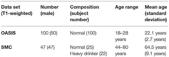
Table 1. Demographic information of OASIS data set and SMC data set used in this study.
Pre-processing
All T1-weighted MR images were passed through pre-processing (Figure 1). Intensity non-uniformity correction (Sled et al., 1998) was followed by brain extraction tool (BET) to extract brain region (Smith, 2002). The images were, then, aligned to the MNI152 average template using an affine transformation of FLIRT of FSL tool (Jenkinson and Smith, 2001; Jenkinson et al., 2002) and the intensities ranged from 2nd to 98th percentiles were normalized to 0 and 255. Since the images were aligned to the standard space, the median slice of x-axis was extracted as MSP and a rectangular region containing CC was cropped. An expert (Gilsoon Park) manually delineated the CC as the gold standard to evaluate the proposed method and the atlas to segment target image. We manually delineated CC according to the protocol suggested by Luders et al. (2005) and Firat et al. (2014). CC in MSP shows clear regions which are splenium, isthmus, posterior body, anterior body, and anterior third. The gold standard images were manually drawn along these regions. We evaluated manually delineated image by measuring intraclass reliability coefficient (ICC). ICC of 0.9931 was obtained for inter-rater reliability (2 raters: Gilsoon Park and Kichang Kwak) and 0.9940 for intra-rater reliability (3 repeats) with 5 Images are randomly selected in each data set.
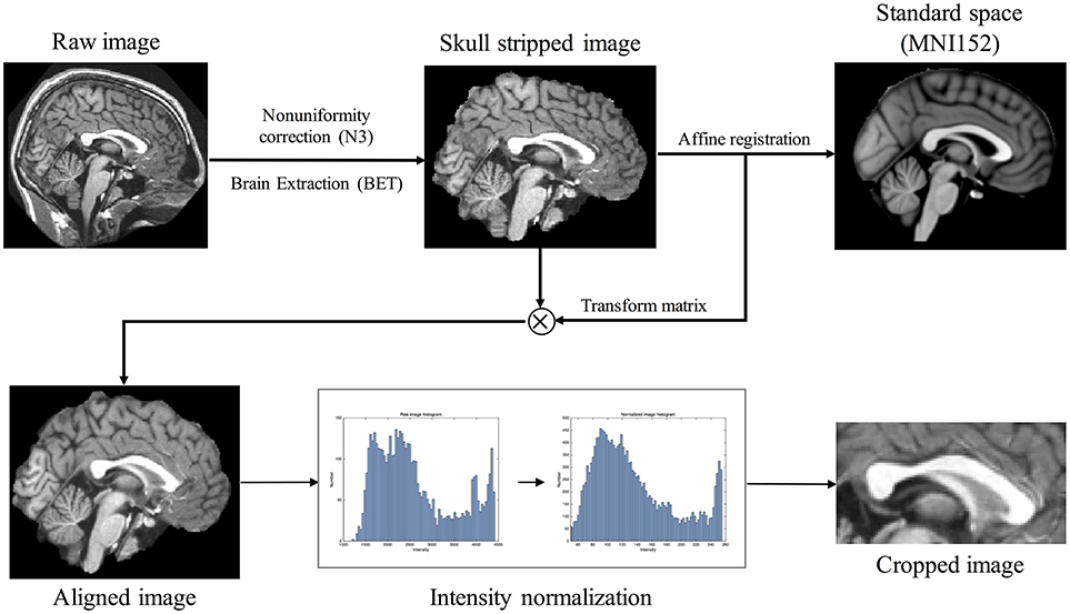
Figure 1. Raw image pre-processing flow chart consisting of the following steps: (1) intensity non-uniformity correction; (2) brain extraction; (3) aligning the image with standard space MNI152 through affine registration; (4) intensity normalization ranging from 0 to 255 using 2nd to 98th percentiles intensities in each image histogram; (5) image cropping in midsagittal plane.
Prior Information Estimated From Multi-Atlas Voting
Multi-atlas voting based segmentation consists of registration and label fusion steps (Figure 2). First, all cropped atlas images were non-linearly registered to a target image, resulting in generation of warping information in each image. Non-linear registration was performed using Automated Image Registration tool (AIR 5.3.0; http://air.bmap.ucla.edu/AIR5/) (Woods et al., 1998). The atlas images and their corresponding label images were aligned to a target image using warping information. The non-linear registration for aligning atlas set to target image is the typical step in multi-atlas voting based segmentation (Aljabar et al., 2009; Wang et al., 2013; Asman et al., 2015). The spatial agreement of the atlas image with the target image is greatly increased due to the non-linear registration, which improves the results of the label fusion. Second, we compared local cross-correlation values between patches, which is a window containing both target voxel and its neighbor voxels on each target voxel location, from aligned atlas images and the target image to choose the subset of atlases. The probability map, overlapping the label images of the subset, was acquired to contain the information of shape and location of CC, which was used as prior information (PIEMV) in the proposed Bayesian framework.
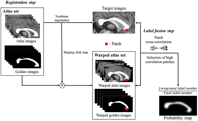
Figure 2. The flow chart of building prior information estimated from multi-atlas voting (PIEMV). This process consists of registration step and label fusion step. In registration step, all cropped atlas images were registered to cropped target image, generating warping field map. Using warping field map, the atlas images and golden images were aligned to a target image. Next label fusion step, the cross-correlation values of patches between target image and aligned atlas images are calculated. Then, the patches with high correlation are selected, generating probability map containing prior information of overall shape and location of corpus callosum of target image.
Likelihood Estimated From Sparse Representation Error
Estimation of sparse representation error was like the method proposed by Mairal et al., but different in the construction of the patch as atom for the dictionary. The patch consisted of image gradient magnitude and direction as well as image intensity because of obvious shape boundary of CC. The LESRE was used in Bayesian inference. We constructed two types of patches: intensity information as only (Old LESRE) and combining gradient information and intensity information together (LESRE) to evaluated how much performance improve by adding gradient information to patch. The process of extracting sparse representation error has the following three steps (Figure 3): (1) the atlas selection step, which selected the subset of the atlases using similarity measurement between atlases and target image; (2) the dictionary construction step, which constructed the dictionary consist sing of the patches extracted from the search region of the selected atlases and extracted the target patch on target image for labeling a target voxel; (3) the sparse representation step, which sparsely represented the target patch as a linear combination of the patches extracted from dictionary using orthogonal matching pursuit (OMP) algorithm.
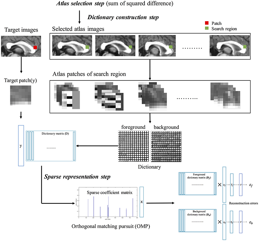
Figure 3. The calculation process of sparse representation error, consisting of atlas selection step, dictionary construction step, and sparse representation step. First, atlas images similar to target image are selected via sum of squared intensity difference. Second, patches are extracted from search region in selected atlas images, constructing atlas patch library. Using label information of atlas golden images, foreground dictionary and background dictionary are generated. Target patch also is extracted from target image. Finally, the target patch is sparsely represented with each patch extracted from the foreground and background dictionaries using orthogonal matching pursuit (OMP) algorithm. The two type reconstructed patches of target patch are used to calculate sparse representation errors.
The atlas selection depending on target image was carried out based on similarity measurement, which was implemented as sum of squared intensity difference in this paper. This selection step reduces computational time and error resulting from naturally individual variation. A search region Ai was defined in each selected atlas image. All patches on the search region were used to construct foreground (i.e., CC) dictionary Df if the center voxel of the patch is labeled foreground, or background dictionary Db otherwise. Finally, we proposed the LESRE based on Wright et al. (2009). The target patch y was represented approximately by the patches dli of dictionary:
where l is the label (i.e., l ∈ {f(foreground), b(background)}), n is the column vector number (i.e., patch number) in each dictionary Dl, xln is weight coefficients. Since sparse representation demand that representation is sparsity, most of weight coefficients xln will be zero. Let , which is sparse coefficient matrix, then the target patch y is also represented as follow:
where εl is reconstruction error that is the difference between target patch and sparse representation. The sparse coefficient matrix Xl can be computed by solving the following L1-norm minimization equation:
Equation (3) consist of L1-norm minimization and L2-norm minimization which indicate sparsity level designated user and searching appropriate column vector representing target patch y as linear combination. This equation can be efficiently solved by OMP algorithm as described in Tropp and Gilbert (2007), which can safely recover signal with sparsity non-zero coefficients. We selected a column vector dln with max projection value on residue rk (initial residue r0 = y) from Dl at each iteration k and obtained a new sparse representation signal consisting of Xlk = {ẋl1, ẋl2, …, ẋlk} and by solving a least squares problems arg ||y − XlkDlk||2, where ẋlk is sparse weight coefficient corresponding to selected column vector . Finally, we updated residue and dictionary matrix by excluding . This procedure was iterated until terminating condition given user. The final residue was the reconstruction error εl and played a key role in LESRE. We compared the reconstruction errors generated from each class, that is, the label of the target patch y based on LESRE only was given as:
The label function L of y patch assigned foreground or background according to minimum εl of y patch over all classes. Note that the l had only two labels consisting of foreground belonging to CC and background in this study.
Bayesian Inference Based Segmentation
The proposed method, Bayesian inference based segmentation (BIbS), combining prior information estimated from multi-atlas voting (PIEMV) containing overall structure information and LESRE containing detailed structure information in the Bayesian framework. Given target patch yi at i th voxel, the Bayesian inference formulation of yi patch is as follow:
where p(cl|yi), posterior probability, is the probability of belonging to class cl via yi, C is class or label number, n is all voxel number in cropped image, p(yi|cl), likelihood, is the probability of observing yi in class-conditional probability distribution according to cl, p(cl), prior probability, is the probability of observing cl reflecting our knowledge of state of nature cl, and p(yi) is evidence which is used to normalize the product of likelihood and prior probability, which does not affect determining the relative probabilities of each class. The class that maximizes the posterior probability is assigned to the target patch yi.
The PIEMV was used as the prior probability in Bayesian inference since it includes pre-defined anatomical knowledge of shape and location of CC. Therefore, the prior probability of observing a class at given patch yi was:
where N is selected atlas number of forming probability map, δ (,) is the Kronecker delta function, and La(i) is the label from the labeled image of a th atlas image at i th voxel. The reconstruction error of LESRE was used as class-conditional probability distribution model using gamma distribution. The gamma distribution reflects the following two properties of the distribution of the error ratio (i.e., foreground error rate/background error rate): (1) the smaller the error ratio generated from label dictionaries, the higher the likelihood of belonging to the label; (2) the frequency of the error ratio close to zero sharply decreases.
where εi is reconstruction error ratio at i th voxel, resulting from sparse representation based on dictionary Dl consisting of error ratios labeled class l and αl is shape parameter and βl is scale parameter in each class. The αl and βl are obtained by reconstruction error ratio set of atlas images we know label. Finally, we labeled the target voxel through comparison of posterior probability:
where Lp of yi patch is labeling function using Bayesian inference at i th voxel. The left and right side of comparison consist of above-mentioned likelihood and prior probability each.
Validation
We used the Dice index (DI), a quantitative measure of the spatial agreement, to evaluate the segmentation accuracy of the proposed method as follows:
where | · | is the number of voxels consisting of positive region in binary segmentation image, and |A∩B| is the number of voxels of common region between A and B binary segmentation image. The binary segmentation images for using DI evaluation are golden standard image made by manual delineation and segmentation result of proposed method. The Dice index range from 0 to 100 percentage, and the value close to 100%indicates the better segmentation performance.
We further evaluated the JLF method (Wang and Yushkevich, 2013; Wang et al., 2013) for CC segmentation and compared our method (BIbS) with JLF in a quantitative and qualitative aspects. JLF improved weighted voting of label fusion step in multi-atlas voting method. The weighed voting of JLF consider pairwise dependency between atlases as explicitly modeled the joint probability of two atlases making a labeling error at a voxel as well as minimizing the total expectation of labeling error (Wang et al., 2013). JLF was conducted using open-source (https://www.nitrc.org/projects/picsl_malf; version 1.3).
The leave-one-out cross validation was performed on each data set to compare the performance of each segmentation method. In OASIS data set, one subject was selected as target image and the other 99 subjects were used as atlas set, and this process was repeated 100 times. In SMC data set, one subject was selected as target image and the other 46 subjects were used as atlas set, and this process was repeated 47 times. A paired t-test was conducted to analyze statistical differences in the Dice index distribution resulting from each method at each data set.
Results
Comparison of Methods
We used leave-one-out cross validation to evaluate segmentation performance, where one subject was selected as target image and the other subjects as atlas image. All method was conducted on each optimal parameter set. The segmentation results of JLF was generated from optimal four primary parameters which are the radius of the image patch (rp), the radius of the search neighborhood (rs), the model parameter for transferring image similarity measures into atlas dependencies (β), and the weight of the conditioning identity matrix added to dependency matrix (α). We set the parameter set according to Wang and Yushkevich (2013), which were rp = 1, rs = 3, β = 2, and α = 0.1 in OASIS data set and rp = 2, rs = 3, β = 2.5, and α = 0.1 in SMC data set. The parameters of PIEMV were the number of atlases and path size. The optimal number of atlases were determined 10 in OASIS and 5 in SMC data set respectively and the optimal path size of both data sets 7 × 7 in PIEMV (Figure S1). The parameters of LESRE were the number of atlases, search region size and path size. The optimal number of atlases was determined 25 and 15, the optimal search region size 7 × 7 and 7 × 7, and the optimal patch size 13 × 13 and 9 × 9 in OASIS and SMC data sets respectively in LESRE (Figure S2). Table 2 shows segmentation results for the mean Dice index and standard deviation in each data set. The table compared the results of the suggested methods with the other methods. In OASIS data set, the results of mean Dice index are that JLF is 96.38 ± 1.78, Old LESRE is 92.96 ± 2.77 (%), LESRE is 94.09 ± 1.82 (%), PIEMV is 95.44 ± 1.58 (%), and BIbS is 95.80 ± 1.52 (%). In SMC data set, the results of mean Dice index are that JLF is 94.99 ± 1.89, Old LESRE is 88.43 ± 4.17 (%), LESRE is 90.71 ± 2.83 (%), PIEMV is 93.4 ± 2.93 (%), and BIbS is 93.72 ± 2.58 (%). Figure 4 shows box plots for the Dice index of each method excepted JLF method in both data sets. The black lines and diamond shapes in box plots are median points and mean points respectively. The Figure 4 indicated BIbS has statistically significant better segmentation performance (p-value in OASIS data set: 7.77e-04, p-value in SMC data set: 0.0436) than both LESRE and PIEMV in both data sets and LESRE has statistically significant better segmentation performance than old LESRE. The segmentation results resulting from SMC data set have the worse segmentation performance than OASIS data set because of variation of CC induced heavy drinkers and old age. The average computation time per image of JLF, PIEMV, LESRE, and BIbS in each optimal parameter set were 10, 68, 124, and 141 s each on a Linux workstation with 2.4 GHz clock speed. JLF was implemented in C language and the other methods were implemented in MATLAB 9.1.0 excepted non-linear registration.
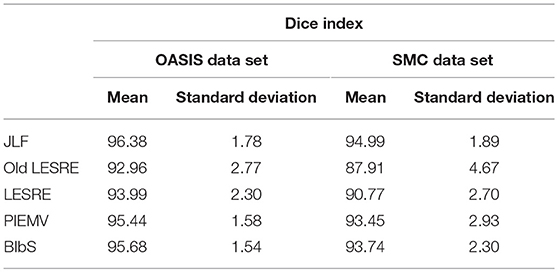
Table 2. Mean Dice index and standard deviation of segmentation results in OASIS data set and SMC data set.
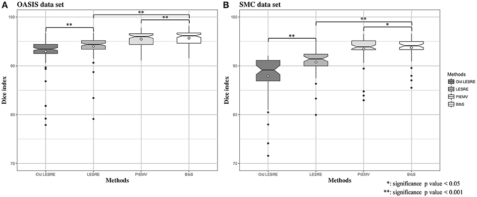
Figure 4. Box plots for Dice index of segmentation results in (A) OASIS data set and (B) SMC data set. In OASIS data set, the results of mean Dice index are that PIEMV is 95.44 ± 1.58 (%), old LESRE is 92.96 ± 2.77 (%), LESRE 93.99 ± 2.30 (%), and BIbS is 95.68 ± 1.54 (%). In SMC data set, the results of mean Dice index are that PIEMV is 93.45 ± 2.93 (%), old LESRE is 87.91 ± 4.67 (%), LESRE is 90.77 ± 2.70 (%), and BIbS is 93.74 ± 2.30 (%). The results indicate two facts that BIbS consisting of multi-atlas voting as prior information and sparse representation error as likelihood has better segmentation performance than the other method with one infromation (i.e., PIEMV and LESRE) and the LESRE with intensity information and gradient information has good segmentation performance than old LESRE with only intensity information.
The Effect of Parameters of BIbS on Segmentation Performance
We investigated the effect of parameters in BIbS, which are the number of atlases, search region, and patch size, on segmentation performance. Figures 5–7 show the relationship between segmentation performance of BIbS (mean Dice index) and the parameters in BIbS. The optimal values of parameters are as follow in both OASIS data set and SMC data set: (1) the number of atlases: 30; (2) search region: 7 × 7; (3) patch size: 13 × 13. In each evaluation, we observed the BIbS performance trend according to target parameter, and the other parameters fixed at optimal values. First, we evaluated the BIbS performance trend according to the number of atlases ranging from 5 to 40 by 5 increments on OASIS data set and SMC data set (Figure 5). The optimal number of atlases with maximum segmentation performance is 30 in both OASIS data set and SMC data set. After the optimal point, the segmentation performance of BIbS decreased. The width of change of mean Dice index about the number of atlases is 0.48 and 1.03 in OASIS data set and SMC data set, respectively. Second, we investigated the effect of search region on BIbS performance. The search region was changed from 3 × 3 to 15 × 15 by 2 × 2 increments. The BIbS performance trend depending on search region was reported in Figure 6. The BIbS performance reached saturation point at 7 × 7 search region in both data sets. The width of change of mean Dice index about the search region is 0.49 and 0.90 in OASIS data set and SMC data set, respectively. Finally, the BIbS performance trend according to patch size was studied on OASIS data set and SMC data set. The patch size was changed from 3 × 3 to 15 × 15 by 2 × 2 increments. Figure 7 shows that the maximum of the BIbS performance according to patch size is 13 × 13 in both OASIS data set and SMC data set. After the maximum point, the segmentation performance of BIbS decreased. The width of change of mean Dice index about patch size is 0.46 and 0.68 in OASIS data set and SMC data set, respectively.
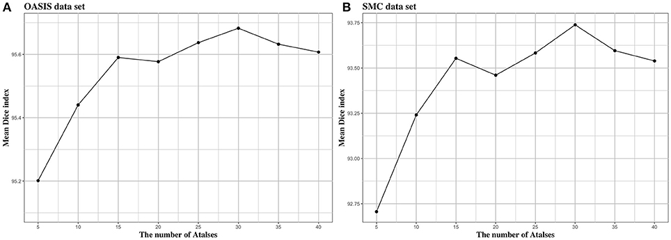
Figure 5. The trend of mean Dice index of BIbS results depending on the number of atlases in (A) OASIS data set and (B) SMC data set. The segmentation performance was evaluated by adjusting the number of atlases from 5 to 40 by 5 increments. The other parameters, search region size, and patch size, are fixed. In both OASIS and SMC data set, the search region size was fixed at 7 × 7 and the patch size was fixed at 13 × 13. The results show that when the number of atlases exceeds a certain number (In both OASIS and SMC data set: 30), the segmentation performance is saturated.
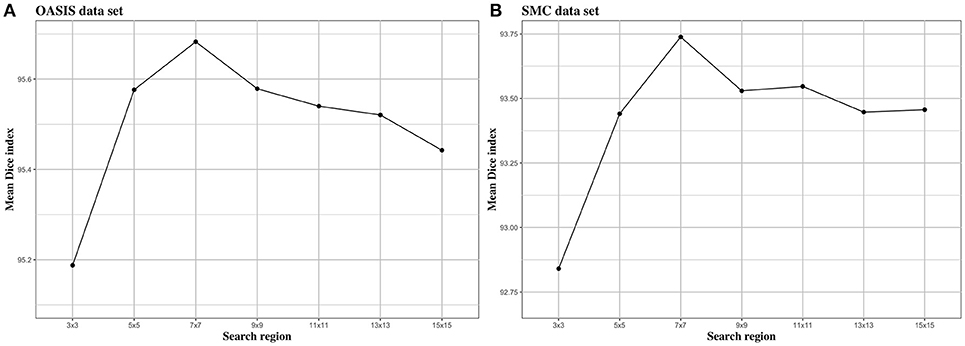
Figure 6. The trend of mean Dice index of BIbS results depending on search region. The segmentation performance was evaluated by adjusting the size of search region from 3 × 3 to 15 × 15 by 2 × 2 increments. The other parameters, atlas selection number and patch size, are fixed. In both (A) OASIS data set and (B) SMC data set, the atlas selection number was fixed at 30 and the patch size was fixed at 13 × 13. The results show that when the search region reaches a certain size [In both (A) OASIS data set and (B) SMC data set: 7 × 7], the segmentation performance is saturated or decreased.
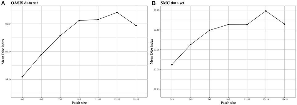
Figure 7. The trend of mean Dice index of BIbS results depending on patch size. The segmentation performance was evaluated by adjusting the size of patch from 3 × 3 to 15 × 15 by 2 increments. The other parameters, atlas selection number and search region size, are fixed. In both (A) OASIS data set and (B) SMC data set, the atlas selection number was fixed at 30 and the search region size was fixed at 7 × 7. The results show that when the patch reaches a certain size [In (A) OASIS data set and (B) SMC data set: 13 × 13], the segmentation performance is saturated.
Images of Segmentation Results of Proposed Method
Figure 8 shows segmentation results of BIbS method in OASIS data set, which consist of best subjects, median subjects, worst subjects, and outlier subjects based on Dice index. From overlap images of outlier subjects and worst subjects, we observed that many false positive occurred because of dilated segmentation results. The top subject of outlier subjects has the noise of bright intensity in the genu of CC, resulting in many false positive. The other false positive shows inter variability problem of manual segmentation rather than showing the problem of the proposed method. In fact, in Figure 8, the segmentation results of all the subjects are robust, but CCs of golden images of the worst subjects and outlier subjects are relatively thin compared to the other subjects. Also, it strongly indicates the inter variability problem of manual segmentation that the most of false positives is generated uniformly along the boundary line of segmentation results in the outlier subjects and worst subjects. Nevertheless, The Dice index of the worst subjects and outlier subjects exceeded 91 and 92%, respectively. In addition, the fornix and noise with intensity like CC were not detected as false positives in segmentation results of other subjects except the top subject of outlier subjects.
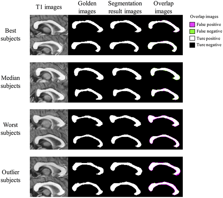
Figure 8. The Segmentation result images of BIbS method in OASIS data set. The images are divided into best subjects, median subjects, worst subjects, and outlier subjects according to Dice index. The overlap images of outlier subjects and worst subjects have many false positive because of dilated segmentation results. The most of false positives result from inter variability problems of manual segmentation because of as follow: (1) the segmentation results of all the subjects are robust, but CCs of golden images of the worst subjects and outlier subjects are relatively thin compared to best subjects and median subjects; (2) the false positive is generated uniformly along the boundary line of the segmentation results in the worst subjects and the outlier subjects.
Discussion
Comparison of Methods
In this paper, we introduced a novel method for the segmentation of CC. From Table 2 and Figure 4, we observed that BIbS had better segmentation performance than both LESRE and PIEMV. It is mean that PIEMV and LESRE are effectively combined on Bayesian inference by improving strengths and weakness of each methods. From comparison of between old LESRE and LESRE, we know that the gradient information significantly improves segmentation performance, since the information reinforce difference between foreground and background for sparse representation. The segmentation performance of SMC data set is relatively lower than OASIS data set because of SMC data set features consisting of elders and heavy drinkers, resulting in variation of CC. But, despite variation of CC the proposed method shows good segmentation performance with 93.74% of mean Dice index.
While JLF had a higher Dice index of about 0.5–1% than BIbS in quantitative aspect, JLF had holes or small regions far from CC that rarely occur in BIbS, which were more frequent and worse in the SMC data set having large CC variation in qualitative aspect (Figure 9). It is important to extract CC as one closed curve since it is generally used as seed for fractional anisotropy (FA) analysis and fiber extraction. Table 3 showed the number of subjects belonging to each value of connected components and Euler number of each method at each data set. If the connected component is not 1, it indicates that the result has a small region far from CC, and if the Euler number is not 1, it indicates that the result has a hole or small region exists. BIbS does not have holes or small regions except only one subject in OASIS data set, but JLF has holes or small regions in many subjects, which are more frequent and worse in SMC data set having large CC variation. The qualitative results of JLF could be improved if proper post-processing is applied or Bayesian framework is adapted to use JLF as prior information. While JLF showed a slightly better quantitative result, our proposed method based on Bayesian framework could be improved by adopting state-of-the-art multi-atlas voting like JLF as prior information.
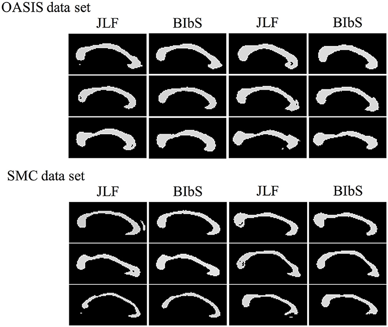
Figure 9. The Segmentation result images of our method (BIbS) and joint label fusion (JLF) method in OASIS data set and SMC data set. JLF creates segmentation image of CC having holes or small region far from CC of ground truth, but these results were disappeared in BIbS method.
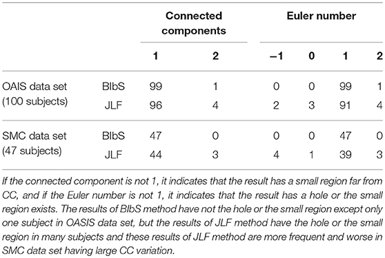
Table 3. The number of subjects belonging to each value of connected components and Euler number of each method at each data set.
The Effect of Parameters of BIbS on Segmentation Performance
We examined the effect of BIbS parameters, which are the number of atlases, search region, and patch size, on segmentation performance (i.e., LESRE parameters included BIbS). The optimization parameter of BIbS in both OASIS and SMC data set is that the atlas selection number is 30, search region size is 7 × 7, and patch size is 13 × 13.
Figures 5–7 described the changes of the segmentation performance of the BIbS depending on each parameters control, and show that the search region has the most influence on segmentation performance in OASIS data set. The search region determines how much the neighborhood patches around the location of the target patch in atlases are included in a dictionary for the sparse representation. As the search region is larger, the patches corresponding to the target patch of target image will be extracted from the atlases and included in the dictionary of foreground or background, resulting in the accuracy of a dictionary for sparse representation is improving. Therefore, the search region should be larger than a certain size (i.e., 3 × 3 in this paper) for the properly working of the sparse representation and if the search region exceeds a certain size (i.e., 7 × 7 in this paper), it no longer has a significant influence on segmentation performance. Figure 6 shows that the segmentation performance of BIbS is increased when the search region is more than a certain size, and the BIbS performance is saturated or decreased by increasing search region.
In Figure 5, the number of atlases most influenced BIbS performance in SMC data set. The number of atlases is associated with the dictionary quality to classify foreground and background. As the number of atlases increases, the atlas less like target image is used and the dictionary consist of various patches, which can improve or worsen segmentation performance. If there are the atlases very similar to a target image, adding the patches from other atlases to the dictionary can reduce segmentation performance. In OASIS data set, the number of subjects is larger than SMC data set and the variations of the CCs are smaller than SMC data set because the OASIS data set consist of normal young people. Therefore, there can be the atlases very similar to the target image in the OASIS data set and using the additional atlases can have slightly better segmentation performance. However, if there is a lot of variations between data like SMC data set, adding the various patches of atlases to the dictionary can improve the segmentation performance. For this reason, Figure 5 shows that the influence of the number of atlases in OASIS data set is lower than in SMC data set.
In Figure 7, patch size slightly influenced BIbS performance in both data sets. The patch size is associated with the spatial information of the patch in the dictionary. The large patch size can improve segmentation performance by adding spatial information to patch, assisting more clear distinction between foreground and background, but can also constitute patch containing unwarranted spatial information. Thus, the patch size, like the number of atlases, has an optimal point depending on the characteristics of the data set. Figure 7 shows that the segmentation performance of BIbS in both data set is increased when the patch size is more than a certain size (i.e., 13 × 13 in this paper), and the BIbS performance is decreased by increasing patch size.
Conclusion
In this paper, we developed a novel method for CC segmentation in MSP, based on Bayesian inference We used reconstruction error resulting from sparse representation as likelihood and probability map generated from multi-atlas voting method as prior information. The segmentation results show that the combination of sparse representation error and multi-atlas voting, based on Bayesian inference, has the significantly better segmentation performance than using each method alone. We also observed that the data set having large CC variation was sensitive to the number of atlases for good segmentation performance. In the future, we will develop a more robust segmentation method about target image having large variation of CC based on Bayesian inference by improving likelihood and prior information and developing framework to effectively search optimal parameters. We will also apply our method to brain structure which is more difficult to segmentation.
Author Contributions
GP and J-ML study concept and design. GP and J-ML drafting of manuscript. GP, KK, and J-ML statistical analysis and interpretation. SS acquisition of samsung medical center dataset.
Funding
This research was supported by the Brain Research Program through the National Research Foundation of Korea (NRF) funded by the Ministry of Science, ICT, & Future Planning (NRF-2014M3C7A1046050); and by the National Research Foundation of Korea (NRF) grant funded by the Korea government (MSIP) (2016R1A2B3016609).
Conflict of Interest Statement
The authors declare that the research was conducted in the absence of any commercial or financial relationships that could be construed as a potential conflict of interest.
The reviewer ML and handling Editor declared their shared affiliation.
Supplementary Material
The Supplementary Material for this article can be found online at: https://www.frontiersin.org/articles/10.3389/fnins.2018.00629/full#supplementary-material
Figure S1. The trend of mean Dice index of PIEMV results depending on the number of atlases and patch size. The segmentation performance was evaluated by adjusting the number of atlases from 5 to 40 by 5 increments and the size of patch from 3 × 3 to 15 × 15 by 2 increments. The other parameters except the test parameter were fixed to the optimal value. The optimal parameter set of PIEMV in OASIS data set was that the number atlases is 10 and the patch size is 7 × 7. The optimal parameter set of PIEMV in SMC data set was that the number atlases is 5 and the patch size is 7 × 7. The results show that the performance of PIEMV in SMC data set having large CC variation was sensitive to the change of the number of atlases and patch size than OASIS data set.
Figure S2. The trend of mean Dice index of LESRE results depending on the number of atlases, search region size, and patch size. The segmentation performance was evaluated by adjusting the number of atlases from 5 to 40 by 5 increments, the size of search region 3 × 3 to 15 × 15 by 2 increments, and the size of patch from 3 × 3 to 15 × 15 by 2 increments. The other parameters except the test parameter were fixed to the optimal value. The optimal parameter set of LESRE in OASIS data set was that the number atlases is 25, the search region size is 7 × 7, and the patch size is 13 × 13. The optimal parameter set of LESRE in SMC data set was that the number atlases is 15, the search region size is 7 × 7, and the patch size is 11 × 11. The change width of performance according to parameter changes is similar in both data sets.
References
Aljabar, P., Heckemann, R. A., Hammers, A., Hajnal, J. V., and Rueckert, D. (2009). Multi-atlas based segmentation of brain images: atlas selection and its effect on accuracy. Neuroimage 46, 726–738. doi: 10.1016/j.neuroimage.2009.02.018
Andreasen, N. C., Rajarethinam, R., Cizadlo, T., Arndt, S., Swayze, V. W., II. Flashman, L. A., et al. (1996). Automatic atlas-based volume estimation of human brain regions from MR images. J. Comput. Assist. Tomogr. 20, 98–106.
Asman, A. J., Huo, Y., Plassard, A. J., and Landman, B. A. (2015). Multi-atlas learner fusion: an efficient segmentation approach for large-scale data. Med. Image Anal. 26, 82–91. doi: 10.1016/j.media.2015.08.010
Balevich, E. C., Haznedar, M. M., Wang, E., Newmark, R. E., Bloom, R., Schneiderman, J. S., et al. (2015). Corpus callosum size and diffusion tensor anisotropy in adolescents and adults with schizophrenia. Psychiatry Res. 231, 244–251. doi: 10.1016/j.pscychresns.2014.12.005
Bookstein, F. L., Streissguth, A. P., Sampson, P. D., Connor, P. D., and Barr, H. M. (2002). Corpus callosum shape and neuropsychological deficits in adult males with heavy fetal alcohol exposure. Neuroimage 15, 233–251. doi: 10.1006/nimg.2001.0977
Caminiti, R., Ghaziri, H., Galuske, R., Hof, P. R., and Innocenti, G. M. (2009). Evolution amplified processing with temporally dispersed slow neuronal connectivity in primates. Proc. Natl. Acad. Sci. U.S.A. 106, 19551–19556. doi: 10.1073/pnas.0907655106
Casanova, M. F., El-Baz, A., Elnakib, A., Giedd, J., Rumsey, J. M., Williams, E. L., et al. (2010). Corpus callosum shape analysis with application to dyslexia. Transl. Neurosci. 1, 124–130. doi: 10.2478/v10134-010-0017-8
Cuadra, M. B., Pollo, C., Bardera, A., Cuisenaire, O., Villemure, J. G., and Thiran, J. P. (2004). Atlas-based segmentation of pathological MR brain images using a model of lesion growth. IEEE Trans. Med. Imaging 23, 1301–1314. doi: 10.1109/TMI.2004.834618
Donoho, D. L. (2006). For most large underdetermined systems of linear equations the minimal Commun. Pure Appl. Math. 59, 797–829. doi: 10.1002/cpa.20132
Doshi, J., Erus, G., Ou, Y., Resnick, S. M., Gur, R. C., Gur, R. E., et al. (2016). MUSE: multi-atlas region segmentation utilizing ensembles of registration algorithms and parameters, and locally optimal atlas selection. Neuroimage 127, 186–195. doi: 10.1016/j.neuroimage.2015.11.073
Elad, M., and Aharon, M. (2006). “Image denoising via learned dictionaries and sparse representation,” in Computer Vision and Pattern Recognition, 2006 IEEE Computer Society Conference on: IEEE (Washington, DC), 895–900.
Elahi, S., Bachman, A. H., Lee, S. H., Sidtis, J. J., Ardekani, B. A., and Alzheimer's Disease Neuroimaging Initiative (2015). Corpus callosum atrophy rate in mild cognitive impairment and prodromal Alzheimer's disease. J. Alzheimers Dis. 45, 921–931. doi: 10.3233/JAD-142631
Elnakib, A., Casanova, M. F., Gimel'farb, G., Switala, A. E., and El-Baz, A. (2012). Dyslexia diagnostics by 3-D shape analysis of the corpus callosum. IEEE Trans. Inf. Technol. Biomed. 16, 700–708. doi: 10.1109/TITB.2012.2187302
Firat, A., Tascioglu, A. B., Demiryurek, M. D., Saygi, S., Karli Oguz, K., Tezer, F. I., et al. (2014). Evaluation of corpus callosum morphometry in patients with mesial temporal lobe epilepsy with hippocampal sclerosis. Surg. Radiol. Anat. 36, 47–54. doi: 10.1007/s00276-013-1144-y
Frazier, T. W., Keshavan, M. S., Minshew, N. J., and Hardan, A. Y. (2012). A two-year longitudinal MRI study of the corpus callosum in autism. J. Autism. Dev. Disord. 42, 2312–2322. doi: 10.1007/s10803-012-1478-z
He, Q., Duan, Y., Miles, J., and Takahashi, N. (2007). A context-sensitive active contour for 2D corpus callosum segmentation. Int. J. Biomed. Imaging 2007:24826. doi: 10.1155/2007/24826
Içer, S. (2013). Automatic segmentation of corpus collasum using Gaussian mixture modeling and Fuzzy C means methods. Comput. Methods Progr. Biomed. 112, 38–46. doi: 10.1016/j.cmpb.2013.06.006
Jenkinson, M., Bannister, P., Brady, M., and Smith, S. (2002). Improved optimization for the robust and accurate linear registration and motion correction of brain images. Neuroimage 17, 825–841. doi: 10.1006/nimg.2002.1132
Jenkinson, M., and Smith, S. (2001). A global optimisation method for robust affine registration of brain images. Med. Image Anal. 5, 143–156. doi: 10.1016/S1361-8415(01)00036-6
Joshi, S. H., Narr, K. L., Philips, O. R., Nuechterlein, K. H., Asarnow, R. F., Toga, A. W., et al. (2013). Statistical shape analysis of the corpus callosum in Schizophrenia. Neuroimage 64, 547–559. doi: 10.1016/j.neuroimage.2012.09.024
Kim, M., Wu, G., Wang, Q., Lee, S. W., and Shen, D. (2015). Improved image registration by sparse patch-based deformation estimation. Neuroimage 105, 257–268. doi: 10.1016/j.neuroimage.2014.10.019
Kim, S. N., Park, J. S., Jang, J. H., Jung, W. H., Shim, G., Park, H. Y., et al. (2012). Increased white matter integrity in the corpus callosum in subjects with high genetic loading for schizophrenia. Prog. Neuropsychopharmacol. Biol. Psychiatry 37, 50–55. doi: 10.1016/j.pnpbp.2011.11.015
Lin, F., Wu, G., Zhu, L., and Lei, H. (2013). Heavy smokers show abnormal microstructural integrity in the anterior corpus callosum: a diffusion tensor imaging study with tract-based spatial statistics. Drug. Alcohol Depend. 129, 82–87. doi: 10.1016/j.drugalcdep.2012.09.013
Liu, M., Zhang, D., Shen, D., and Alzheimer's Disease Neuroimaging Initiative (2012). Ensemble sparse classification of Alzheimer's disease. Neuroimage 60, 1106–1116. doi: 10.1016/j.neuroimage.2012.01.055
Luders, E., Narr, K., Zaidel, E., Thompson, P., Jancke, L., and Toga, A. (2005). Parasagittal asymmetries of the corpus callosum. Cereb. Cortex 16, 346–354. doi: 10.1093/cercor/bhi112
Mairal, J., Elad, M., and Sapiro, G. (2008). Sparse representation for color image restoration. IEEE Trans. Image Process. 17, 53–69. doi: 10.1109/TIP.2007.911828
Marcus, D. S., Wang, T. H., Parker, J., Csernansky, J. G., Morris, J. C., and Buckner, R. L. (2007). Open Access Series of Imaging Studies (OASIS): cross-sectional MRI data in young, middle aged, nondemented, and demented older adults. J. Cogn. Neurosci. 19, 1498–1507. doi: 10.1162/jocn.2007.19.9.1498
O'Dwyer, R., Wehner, T., LaPresto, E., Ping, L., Tkach, J., Noachtar, S., et al. (2010). Differences in corpus callosum volume and diffusivity between temporal and frontal lobe epilepsy. Epilepsy Behav. 19, 376–382. doi: 10.1016/j.yebeh.2010.06.049
Patenaude, B., Smith, S. M., Kennedy, D. N., and Jenkinson, M. (2011). A Bayesian model of shape and appearance for subcortical brain segmentation. Neuroimage 56, 907–922. doi: 10.1016/j.neuroimage.2011.02.046
Prigge, M. B., Lange, N., Bigler, E. D., Merkley, T. L., Neeley, E. S., Abildskov, T. J., et al. (2013). Corpus callosum area in children and adults with autism. Res. Autism Spectr. Disord. 7, 221–234. doi: 10.1016/j.rasd.2012.09.007
Sanroma, G., Wu, G., Gao, Y., Thung, K. H., Guo, Y., and Shen, D. (2015). A transversal approach for patch-based label fusion via matrix completion. Med. Image Anal. 24, 135–148. doi: 10.1016/j.media.2015.06.002
Shyu, K. K., Pham, V. T., Tran, T. T., and Lee, P. L. (2012). Unsupervised active contours driven by density distance and local fitting energy with applications to medical image segmentation. Mach. Vis. Appl. 23, 1159–1175. doi: 10.1007/s00138-011-0373-5
Sled, J. G., Zijdenbos, A. P., and Evans, A. C. (1998). A nonparametric method for automatic correction of intensity nonuniformity in MRI data. IEEE Trans. Med. Imaging 17, 87–97. doi: 10.1109/42.668698
Smith, S. M. (2002). Fast robust automated brain extraction. Hum. Brain Mapp. 17, 143–155. doi: 10.1002/hbm.10062
Tong, T., Wolz, R., Coupé, P., Hajnal, J. V., Rueckert, D., and Alzheimer's Disease Neuroimaging Initiative (2013). Segmentation of MR images via discriminative dictionary learning and sparse coding: application to hippocampus labeling. Neuroimage 76, 11–23. doi: 10.1016/j.neuroimage.2013.02.069
Tropp, J. A., and Gilbert, A. C. (2007). Signal recovery from random measurements via orthogonal matching pursuit. IEEE Trans. Inf. Theor. 53, 4655–4666. doi: 10.1109/TIT.2007.909108
Wang, H., Suh, J. W., Das, S. R., Pluta, J. B., Craige, C., and Yushkevich, P. A. (2013). Multi-atlas segmentation with joint label fusion. IEEE Trans. Pattern Anal. Mach. Intell. 35, 611–623. doi: 10.1109/TPAMI.2012.143
Wang, H., and Yushkevich, P. A. (2013). Multi-atlas segmentation with joint label fusion and corrective learning-an open source implementation. Front. Neuroinform. 7:27. doi: 10.3389/fninf.2013.00027
Wang, X. D., Ren, M., Zhu, M. W., Gao, W. P., Zhang, J., Shen, H., et al. (2015). Corpus callosum atrophy associated with the degree of cognitive decline in patients with Alzheimer's dementia or mild cognitive impairment: a meta-analysis of the region of interest structural imaging studies. J. Psychiatr. Res. 63, 10–19. doi: 10.1016/j.jpsychires.2015.02.005
Warfield, S. K., Zou, K. H., and Wells, W. M. (2004). Simultaneous truth and performance level estimation (STAPLE): an algorithm for the validation of image segmentation. IEEE Trans. Med. Imaging 23, 903–921. doi: 10.1109/TMI.2004.828354
Woods, R. P., Grafton, S. T., Watson, J. D., Sicotte, N. L., and Mazziotta, J. C. (1998). Automated image registration: II. intersubject validation of linear and nonlinear models. J. Comput. Assist. Tomogr. 22, 153–165. doi: 10.1097/00004728-199801000-00028
Wright, J., Yang, A. Y., Ganesh, A., Sastry, S. S., and Ma, Y. (2009). Robust face recognition via sparse representation. IEEE Trans. Pattern Anal. Mach. Intell. 31, 210–227. doi: 10.1109/TPAMI.2008.79
Yang, M., and Zhang, L. (2010). “Gabor feature based sparse representation for face recognition with gabor occlusion dictionary,” in Computer Vision–European Conference on Computer Vision 2010 (Berlin; Heidelberg: Springer), 448–461.
Yeo, S. Y., Xie, X., Sazonov, I., and Nithiarasu, P. (2014). Segmentation of biomedical images using active contour model with robust image feature and shape prior. Int. J. Numer. Methods Biomed. Eng. 30, 232–248. doi: 10.1002/cnm.2600
Zhang, Y., Caspers, S., Fan, L., Fan, Y., Song, M., Liu, C., et al. (2015). Robust brain parcellation using sparse representation on resting-state fMRI. Brain Struc. Funct. 220, 3565–3579. doi: 10.1007/s00429-014-0874-x
Keywords: corpus callosum, segmentation, sparse representation, multi-atlas voting, Bayesian inference
Citation: Park G, Kwak K, Seo SW and Lee J-M (2018) Automatic Segmentation of Corpus Callosum in Midsagittal Based on Bayesian Inference Consisting of Sparse Representation Error and Multi-Atlas Voting. Front. Neurosci. 12:629. doi: 10.3389/fnins.2018.00629
Received: 06 January 2018; Accepted: 21 August 2018;
Published: 11 September 2018.
Edited by:
Jussi Tohka, University of Eastern Finland, FinlandReviewed by:
Mengting Liu, University of Southern California, United StatesJin Gahm, University of Southern California, United States
Copyright © 2018 Park, Kwak, Seo and Lee. This is an open-access article distributed under the terms of the Creative Commons Attribution License (CC BY). The use, distribution or reproduction in other forums is permitted, provided the original author(s) and the copyright owner(s) are credited and that the original publication in this journal is cited, in accordance with accepted academic practice. No use, distribution or reproduction is permitted which does not comply with these terms.
*Correspondence: Jong-Min Lee, ljm@hanyang.ac.kr