Image quality analysis of high-density diffuse optical tomography incorporating a subject-specific head model
- 1 School of Computer Science, University of Birmingham, Birmingham, UK
- 2 Department of Radiology, Washington University School of Medicine, St. Louis, MO, USA
High-density diffuse optical tomography (HD-DOT) methods have shown significant improvement in localization accuracy and image resolution compared to traditional topographic near infrared spectroscopy of the human brain. In this work we provide a comprehensive evaluation of image quality in visual cortex mapping via a simulation study with the use of an anatomical head model derived from MRI data of a human subject. A model of individual head anatomy provides the surface shape and internal structure that allow for the construction of a more realistic physical model for the forward problem, as well as the use of a structural constraint in the inverse problem. The HD-DOT model utilized here incorporates multiple source-detector separations with continuous-wave data with added noise based on experimental results. To evaluate image quality we quantify the localization error and localized volume at half maximum (LVHM) throughout a region of interest within the visual cortex and systematically analyze the use of whole-brain tissue spatial constraint within image reconstruction. Our results demonstrate that an image quality with less than 10 mm in localization error and 1000 m3 in LVHM can be obtained up to 13 mm below the scalp surface with a typical unconstrained reconstruction and up to 18 mm deep when a whole-brain spatial constraint based on the brain tissue is utilized.
Introduction
Diffuse optical tomography (DOT) of the human brain is an emerging neuroimaging methodology that allows continuous non-invasive imaging of human brain functional activity by taking near infrared (NIR) optical measurements using sources and detectors placed on the human scalp (Bluestone et al., 2001; Boas et al., 2004b; Gibson et al., 2006; Zeff et al., 2007; White et al., 2009; Custo et al., 2010; Koch et al., 2010; White and Culver, 2010a; Niu et al., 2011). While most hemodynamic-based neuroimaging research studies in healthy adult subjects are conducted with functional magnetic resonance imaging (fMRI), its relative high cost, fixed scanner locations, physical constraints during imaging and its inability [through the Blood Oxygen Level Dependant (BOLD) signal] to comprehensively provide or assess altered brain metabolism, limit fMRI’s translation as a bedside clinical tool. DOT is emerging as a non-invasive neuroimaging modality that is uniquely suited to this setting, as it is a mobile system utilizing a small, flexible imaging cap (Obrig and Villringer, 2003). It also has the potential to measure absolute changes in oxygenated (ΔHbO2), deoxygenated (ΔHbR), and total hemoglobin (ΔHbT), providing more comprehensive images of the brain’s hemodynamics (Boas et al., 2004b; Pogue et al., 2006).
Recently high-density diffuse optical tomography (HD-DOT) systems have been developed to provide high spatial sampling of the brain tissue using a large number of overlapping measurements. Initial efficacy of HD-DOT has been demonstrated in vivo with studies that include retinotopic mapping of adult human visual cortex (Zeff et al., 2007; Eggebrecht et al., 2012), somatotopic mapping of the sensor motor cortex (Koch et al., 2010), resting-state mapping of functional connectivity (White et al., 2009), and phase-encoded retinotopic mapping (White and Culver, 2010a). The HD-DOT images have a level of detail that was previously inaccessible via sparse functional near-infrared spectroscopy (fNIRS) arrays (White and Culver, 2010b). However most of these initial HD-DOT studies have been either limited by the use of simplified generic head models, or have only considered a limited number of simulated focal activations within the visual cortex. In this work, we expand the problem of recovered image analysis from these limitations to encompass the entire visual cortex using a subject specific anatomical model. Additionally we introduce and utilize robust image analysis metrics that allow a comprehensive study of the entire visual cortex, thereby providing a better understanding of the HD-DOT imaging performance.
Following advances in DOT breast cancer imaging (Brooksby et al., 2005; Dehghani et al., 2009a), more recent DOT studies of brain function have begun to use magnetic resonance imaging (MRI)-guided approaches in which a three-dimensional (3D) anatomical head model is constructed (Boas and Dale, 2005). The realistic representation of the physical model provides the necessary external and internal structure necessary for an accurate description of light propagation in tissue. Furthermore the realistic head model also provides a possibility for incorporating anatomically derived spatial constraints (Boas and Dale, 2005). Recently the performance of HD-DOT was evaluated by Dehghani et al. (2009b) and Heiskala et al. (2009b) with anatomically realistic head models. However neither study provided a quantitative evaluation of the point-spread-function (PSF) throughout the entire field of view (FOV) as conducted by Boas et al. (2004a) and White and Culver (2010b) which themselves were limited to simplified head models. This paper provides a fully comprehensive quantification of the PSF for HD-DOT using an anatomically realistic head, both with and without an anatomically based whole-brain spatial constraint for image recovery. Specifically, PSF analysis is performed throughout the visual cortex within a specified region of interest (ROI), corresponding to the total field of view of an experimental HD-DOT system (Zeff et al., 2007).
Materials and Methods
Head Model
In order to guide the physical modeling of a subject-specific human head, T1-weighted MPRAGE [echo time (TE) = 3.13 ms, repetition time (TR) = 2400 ms, flip angle = 8°, 1 mm × 1 mm × 1 mm isotropic voxels] and T2-weighted (TE = 84 ms, flip angle = 120°, 1 mm × 1 mm × 4 mm voxels) scans of the same subject were collected on a Siemens Trio (Erlangen, Germany) 3T scanner at Washington University School of Medicine. The subject passed MR screening to ensure their safe participation. Informed consent was obtained and the research was approved by the Human Research Protection Office at Washington University School of Medicine. In-house automated algorithms were applied to both MRI dataset, which performs a series of iterative thresholding, region growing, and masking technique to produce a set of segmented images that indicate scalp, skull, cerebrospinal (CSF), gray matter, and white matter in different grayscale, as shown in Figure 1. These three-dimensional images were then imported in the Mimics software package (Materialise, http://www.materialise.com/mimics) to create a three-dimensional finite element head model (FEM). The model was composed of 1,087,223 nodes corresponding to 6,289,566 linear tetrahedral elements with maximum inter nodal distance of 1 mm. Each node was labeled by one of the five segmented head tissue types as stated above. Alternative methods for tissue segmentation through the use of statistical methods based on a template of the brain atlas can also be utilized and may prove to be more suitable when dealing with multiple subjects while reducing operator bias. Tissue optical properties assigned to the head model were values estimated at 750 nm (Table 1), which is one of the primary wavelengths used in our current system (White and Culver, 2010b) and can be adapted to other wavelengths and spectral analysis. These values were estimated by applying a linear line-fitting scheme on values published at other available wavelengths (Bevilacqua et al., 1999; Strangman et al., 2003; Custo et al., 2006).
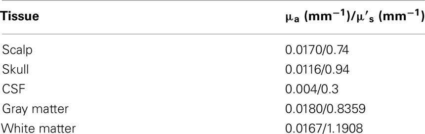
Table 1. Tissue optical properties at 750 nm.
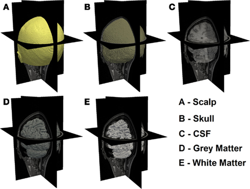
Figure 1. Three-dimensional surface rendered view for each of the five segmented head tissues.
Optode Array Arrangements
The high-density (HD) imaging array used for the data simulation consisted of 24 sources and 28 detectors, which has been previously described (Zeff et al., 2007; White and Culver, 2010b). The HD imaging array was modeled on the scalp surface over the visual cortex as shown in Figures 2A,B. Within this context, nearest neighbor measurements can be defined based on source-detector separations, Figure 2C. In this study all detectors within 40 mm from each source (i.e., first, second, and third nearest neighbors have distances of 13, 30, and 40 mm respectively) were utilized, giving rise to a total of 260 independent measurements. It was assumed that only intensity data (as available from a continuous-wave system) measured at 750 nm were used to provide maps of optical absorption related changes only. A ROI was defined as the volume up to 40 mm under the posterior field of view (FOV) of the HD imaging array, as shown in Figure 2B. The posterior FOV has been selected to focus on the visual cortex region under the array with the highest sensitivities and lowest image artifacts (White and Culver, 2010b).

Figure 2. (A) Posterior and (B) lateral schematic view showing the placement of the imaging array over the visual cortex of the head model with 24 sources (red squares) and 28 detectors (blue circles). A region of interest (ROI) was defined by the volume enclosed within the black solid rectangle, (C) first to third nearest neighbor measurements defined by separation of 13, 30, 40 mm respectively within the context of the HD imaging array.
Forward Light Modeling
Forward modeling of light propagation within the head model was performed using NIRFAST (Dehghani et al., 2008) which is a modeling and image reconstruction toolbox based on the Diffusion Approximation. NIRFAST was used to generate a sensitivity matrix J (also known as the Jacobian or Weight matrix) which represents the changes of measured “boundary data” Δy due to a small spatial perturbation in absorption Δx, given an initial model of baseline optical properties. The forward problem of the head model can thus be expressed as:
where Jh is a matrix with a size of number of measurements (NM) by number of nodes (NN), Δx is a vector of length NN and Δy is a vector of length NM. Since Δx corresponds to a small change in absorption from an initial baseline state, Δy is the corresponding change in amplitude of the measured signal, i.e. Δy = y – yo, where yo is the initial rest state measurement and y is the measurement after a change in absorption. In this work the sensitivity matrix reflected the logarithmic change in the measured data, such that Δy = log(y) – log(yo) = log(y/yo), which is the Rytov approximation (Arridge, 1999) and has shown to allow for the large dynamic range of the measurements (O’Leary, 1996).
Inverse Problem
The aim of image reconstruction is the recovery of the optical parameter Δx at each FEM node within the domain using measurements Δy. Since Jh in Eq.1 is non-invertible, the Moore–Penrose generalized inverse (Penrose, 1955) was applied in the inverse problem to provide the least squares solution:
where α2 is a regularization factor and is the spatially regularized sensitivity given by
where β is the spatial regularization factor. This scheme is applied to regularize the hyper sensitivities often observed in regions near the optodes (Boas and Dale, 2005; Li et al., 2011), allowing a more homogenous spatial distribution of the sensitivity. The optimal values chosen in this work were α = 10−2 × the maximum singular value of Jh, and β = 10−2, which were found to provide good imaging metrics based on values used in our previous human (White and Culver, 2010b) and animal (Culver et al., 2003) DOT studies.
Based on the spatial a priori information, the sensitivity matrix Jh can be segmented into two parts such that Jb contains the sensitivities of all the nodes in the brain (white and gray matter) and Jnb includes the sensitivities of all the nodes not belonging to the brain (CSF, skull, and scalp). In order to constrain the image recovery problem to nodes that are only associated with the brain, Jb can be used instead of Jh in the spatial-regularization step, Eq.3, and consequently Eq.2. The use of whole-brain constraint in image reconstruction in this study is similar to the cortical constraint applied by (Boas and Dale, 2005) which limits the recovered activation to only the gray matter. However a key issue with the cortical constraint is that it requires accurate subject-specific gray matter segmentation. In comparison, the whole-brain constraint as applied in this work should, in principal, be more robust with respect to tissue segmentation errors, gray and white matter specifically. Subsequently model mismatch errors due to gray and white matter segmentation should be minimized which are common issues with the incorporation of structural a priori information within in vivo DOT.
Total Spatially Regularized Sensitivity
The total spatially regularized sensitivity (for either or ) is calculated as the sum of the spatially regularized sensitivity over all measurement pairs at each spatial node within the head model. This is effectively the sum of the elements in each column of the spatially regularized sensitivity matrix :
where is the total spatially regularized sensitivity at node j, and is the spatially regularized sensitivity at node j due to source-detector pair measurement i for a total number of NM measurements. This provides a measure of the system’s sensitivity profile throughout the imaging domain.
Point-Spread-Function Analysis
In order to evaluate image quality, point-spread-function (PSF) analysis was performed at each of the 40,281 gray matter (visual cortex) nodes within the ROI as defined in Section “Optode Array Arrangements” and Figures 2A,B. The simulated absorptive perturbation, Δx, was assumed to come from a small (a single node, corresponding to 1 mm3, given that the FEM model consists of spatial node distribution of 1 mm resolution) focal hemodynamic visual response located within the visual cortex. The magnitude of perturbation at the gyri of the cortical surface was determined to match the acquired measurement in in vivo studies within the visual cortex (Zeff et al., 2007), and was kept constant for all subsequent perturbations deeper within the brain. For each simulated focal activation, Eq.1 was used to compute the noiseless data (Δy-noiseless). In line with our current in vivo performance, 0.1, 0.14, and 1% Gaussian random noise was added to first, second, and third nearest neighbor measurements to provide realistic data, Δy. In order to mimic our current data collection strategy, for each focal activation, 10 sets of noise added data were generated which were then appropriately averaged and images of each focal activation were reconstructed with and without the application of whole-brain constraint.
Metrics of Image Quality
Consider an example target and two reconstructed activations as shown in Figure 3. It is clearly evident that in Case A, whereby a single activation has been recovered, the use of localization error (displacement between actual and recovered peak value) is an intuitive and commonplace image quality metric. Additionally for Case A, the use of full volume half maximum (FVHM) is an appropriate evaluation of the spread (size) of the recovered parameter. There exists however scenarios, such as demonstrated in Case B, whereby multiple activations are reconstructed, instead of the expected single activation. As such the use of localization error and FVHM alone is not straightforward, since it is not clear which recovered activation should be used for accurate analysis. To this end, we will next define and clearly state the specific image quality metrics utilized in this work, which aims to minimize the uncertainty due to multiple recovered activations.
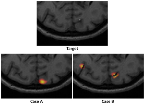
Figure 3. An example of a “target” focal activation on the cortical surface and two examples of reconstructed activations: Case A where a single activation is recovered and Case B where multiple activations are recovered.
Following from above, three metrics were utilized to provide a quantitative measure of the imaging performance. First the localized full volume half maximum (LVHM) was defined as the single volume enclosing the peak-response node in the PSF as well as other contiguous nodes having a value above half of the peak response. In case A of Figure 3, this would correspond to the FVHM of the single recovered activation, whereas in Case B, it corresponds to a single volume containing the peak-response node. Second, the localization error was defined as the Euclidian difference between the peak-response node in the LVHM (also PSF) and the target node:
where (x, y, z) represents the nodal coordinate in the standard x-y-z 3D coordinate system. By such definitions it is assumed that the LVHM reveals useful localization information about the actual target, which may not be valid when multi-regional artifacts are reconstructed due to low sensitivity and/or poor signal to noise ratio (SNR). Since the presence of imaging artifacts could affect the integrity of the localization error and LVHM as quantified above, we also introduced the third metric “focality,” given by:
where full volume half maximum (FVHM) is defined as the total (sum) volume of all nodes having a value above half of the maximum reconstructed response. While a focality of 1 indicates a single-regional PSF, a focality value above 0.5 describes a reconstructed activation well separated from the background artifacts, assuring a good level of integrity in the corresponding localization error and LVHM. As in Case A of Figure 3, the focality value clearly is equal to 1, whereas in Case B, it would correspond to a value of less than 1. Since a reasonable objective within the field of neuroimaging is 10 mm resolution, we set the maximum tolerance for localization error at 10 mm, and 1000 mm3 for LVHM (White and Culver, 2010b).
Results
Total Spatially Regularized Sensitivity
Figure 4 shows the spatial distribution of the total spatially regularized sensitivity (from Eq.4) with the full head (left column “Head”) and with a whole-brain constraint (right column “Brain”) at three different axial slices with different positions relative to sources and detectors. Since the spatial distribution of sensitivity is highly dependent on optode placements, variations are expected between the slices when utilizing sparse optode placement. In Figure 4 however the three sensitivity distributions within the same column show similar spatial coverage owing to the high spatial sampling of tissue by a large number of overlapping measurements and the spatial regularization scheme applied in Eq.3. Without using a whole-brain constraint, the regions with larger than 50% sensitivity (indicated by warm color in Figure 4) reside mainly within the scalp, skull and CSF, which is a distribution not ideally suitable for imaging visual cortex activations that take place in the gray matter. While the gyri are also well covered by high sensitivity, sulcal folds show a significant decrease in sensitivity.
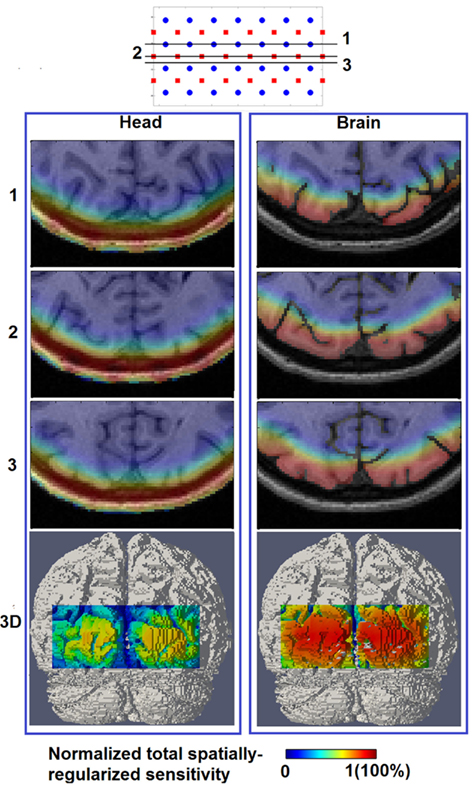
Figure 4. Total spatially regularized sensitivity (normalized to 1) [column (Head)] and [column (Brain)] are shown at three axial MRI slices (1, 2, and 3) with different positions relative to sources and detectors, and also at posterior view on the 3D cortical surface (bottom row).
On the other hand the use of a whole-brain constraint produces a more gradual decay of sensitivity in the brain region as depth increases. The sensitivity profile throughout the gray matter is more uniform with the whole-brain constraint, potentially indicating a better recovery of focal activations within the visual cortex both in the sulcal folds and gyri.
Metrics of Image Quality
Figure 5 (Head) shows the color-coded scatter plots of the three defined imaging performance metrics (localization error, LVHM, and focality) versus imaging depth for all the PSFs (40,281 individual focal activations from the gray matter (visual cortex) nodes within the ROI) obtained using full head (non-constrained) reconstruction. The color-coded plots have been utilized to identify the cases whereby the localization error is either less than 10 mm (green) or greater than 10 mm (red). From these Figures, a “high image quality zone” between 9 mm and 13 mm imaging depth can be identified, where localization error increases from (0.72 ± 0.62) to (2.67 ± 2.54) mm, LVHM increases from (578 ± 64) to (842 ± 185) mm3, indicating that the upper boundary of the “mean ± standard deviation” window for both metrics (specifically the LVHM) are below or roughly equal to its specified tolerance level. Beyond 13 mm depth there is a growing number of poor quality PSFs (red dots) appearing in the form of high localization error, low LVHM and more crucially lower focality, indicating a gradual takeover by imaging artifacts due to poor signal to noise ratio at these higher depths.
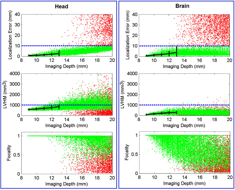
Figure 5. Scatter plot of localization error, LVHM and focality versus imaging depth (up to 20 mm) for all PSFs reconstructed with full head [column (Head)] and brain constraint [column (Brain)]. Each dot, which represents a reconstructed PSF, is color-coded in green if its localization error is less than 10 mm or otherwise in red. The mean ± standard deviations are reported at 1.0 mm imaging depth interval (black solid plot) up to 13 mm. The blue dashed line in each figure represents tolerance level for each metric as stated in Section “Metrics of Image Quality.” In all cases the x-axis has been limited to 20 mm for conciseness.
Figure 6 (Head) shows the spatial distribution of localization errors up to 10 mm on top of the corresponding MRI, where the white solid and dashed lines represents a depth of 13 mm and 18 mm below the scalp, respectively. These data points have high integrity as all of the displayed results have a focality above 0.5 as evident in Figure 5 (Head). A key observation in Figure 6 (Head) is that although the localization error is low and constant at depths of up to 13 mm, it increases with imaging depth.
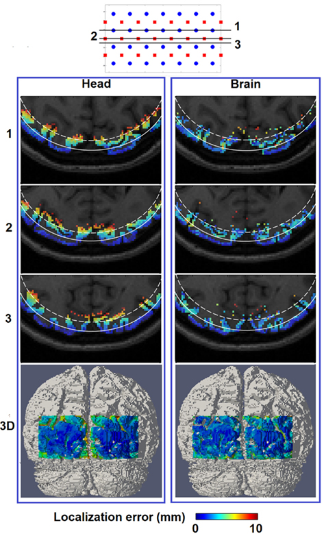
Figure 6. Spatial distribution of localization error for image reconstruction with the full head [column (Head)] and a brain constraint [column (Brain)] are shown at three axial MRI slices (1, 2, and 3) with different positions relative to sources and detectors, as well as a posterior view on the 3D cortical surface (bottom row). The white solid contour on each MRI slices represents imaging depth of 13 mm below the scalp while the white dashed contour represents imaging depth of 18 mm below the scalp.
Figure 5 (Brain) shows the same scatter plots of the three metrics using the whole-brain constrained reconstruction. The “high image quality zone” in this case can also be identified as between 9 mm to 13 mm below the scalp, where localization error increases from (0.54 ± 0.67) mm to (3.85 ± 5.98) mm, and LVHM increases from (96 ± 43) to (286 ± 120) mm3. While the focality plot is given, it is important to note that the 0.5 focality tolerance may not be directly applicable in this case, since the PSF is constrained to the gray and white matter only. In cases where the focal activation lies within a fold of the visual cortex, the recovered activation using the whole-brain constrain may be “split” across this fold, thereby decreasing the calculated “focality” metric [see Y in Figure 8 (Brain) for an example].
Figure 6 (Brain) shows that localization error of less than 10 mm covers up to 18 mm below the scalp surface with better and more uniform localization accuracy beyond the 13 mm contour as compared to Figure 6 (Head), owing to the improved depth localization. It is worth noting the existence of minor variations in localization accuracy between spatial locations of the same depth, as noticed in Figure 6 (Brain), which is likely to be the result of the complicated physical structure of the brain (and therefore the applied constraint), due to the folds of the brain.
Figure 7 shows the spatial distribution of LVHM up to 1000 mm3 on top of the corresponding MRI, where the white solid and dashed lines represent a depth of 13 mm and 18 mm below the scalp respectively. In the case of using non-constrained reconstruction, there exists a high magnitude and a non-uniform variation of LVHM within the gray matter, whereas the application of “whole-brain” constrained image reconstruction dramatically reduces the magnitude of the LVHM and provides a much more uniform degree of parameter recovery throughout the visual cortex. This is substantially evident in the 3D cortical surface maps (Figure 7, bottom row), which is inline with the scatter plots shown in Figure 5.
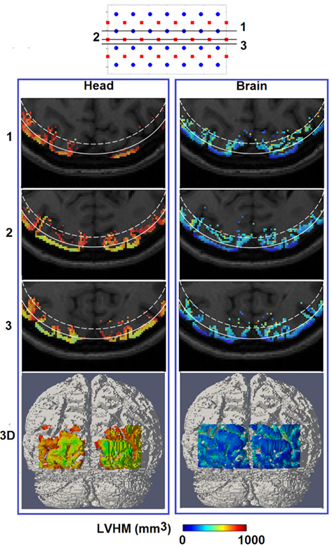
Figure 7. Same as Figure 6, but for spatial distribution of localized volume half maximum.
Discussion
In this study we have presented a routine for conducting subject-specific HD-DOT studies and quantitatively evaluated the corresponding image performance throughout a ROI within the visual cortex. The first step is to construct a high-resolution 3D finite element head model that incorporates realistic tissue spatial information (Figure 1), which requires both T1 and T2 MRI data set from the subject and an appropriate tissue segmentation procedure. Compared with using simplified generic head models (Zeff et al., 2007; White et al., 2009; White and Culver, 2010a,b) this approach reduces the systematic imaging error due to mismatch between in vivo and computational models. After a spatial regularization scheme is applied, the full head total sensitivity is shown to have high sensitivities (larger than 50% of maximum value) covering non-brain regions and no further than superficial regions of the cortex [Figure 4 (Head)]. This reveals a deeper sensitivity coverage than the Dehghani et al. (2009b) study which reported total sensitivity on the cortical surface at 10% of maximum value. However the head model used in that study was based on fewer segmented regions, which were also less complex in structure.
The reconstructed PSF for each gray matter node within the ROI is evaluated by three metrics of image quality. Traditionally FVHM and localization error have been the standard metrics for evaluating imaging quality. We have demonstrated that in presence of noise where multi-regional activations are reconstructed, the FVHM may not be the best parameter as it is not trivial to isolate the true recovered activation from background noise and artifacts. Therefore we have introduced two parameters LVHM and focality that aim to provide more information regarding the image quality. We have found that in presence of noise these parameters provide a more consistent evaluation of image quality when used in conjunction with localization error, as compared to FVHM and localization error alone.
A “high quality region” down to 13 mm imaging depth below the scalp is identified Figure 5 (Head) based on defined thresholds of each image quality metric. Localization error and FWHM (as derived from LVHM) at 10 mm imaging depth are (0.86 ± 0.67) mm and (10.6 ± 0.4) mm respectively, which are within good agreement with White and Culver (2010b) findings on a simplified head model.
When a whole-brain constraint is applied within the image recovery algorithm, the total sensitivity yields a more homogenous spread of sensitivities on the 3D cortical FOV [Figure 4 (Brain)]. Consequently focal activation up to 18 mm below the scalp can potentially be better localized as shown quantitatively by metrics of image quality in Figure 6 (Brain). This improvement in localization with depth (from 13 mm without whole-brain constraint to 18 mm with whole-brain constraint) has not been evaluated in any other previous study, highlighting the utility and benefit of the proposed scheme.
If an image quality goal is set at less than 10 mm localization accuracy (and image resolution), these comprehensive simulations suggest that HD-DOT is capable of imaging focal activations within the visual cortex up to 13 mm below the scalp using full head reconstruction [Figures 6 and 7 (Head)], and up to 18 mm using whole-brain constrained reconstruction [Figures 6 and 7 (Brain)]. Both depths roughly correspond to the 30% contour in their respective total spatially regularized sensitivity (Figure 4).
It can be observed that the lack of a spatial constraint pulls the activations toward the surface to regions of higher sensitivity, sacrificing 5 mm imaging depth capability and image resolution which is also in line with a previous study (Boas and Dale, 2005). Such a phenomenon has been qualitatively demonstrated in Figure 8 (Head): while a perturbation moves from location X to Z, its recovered location stops moving beyond the 13 mm contour. Effectively at location Z the PSF is been pulled toward the skull/scalp region where the sensitivity is much higher [see Figure 4 (Head)]. Thus such decrease in localization accuracy represents a stronger effect on the depth accuracy than the lateral localization accuracy. On the other hand, localization errors at given specific depths (regardless of lateral locations), show good consistency as shown in Figure 6 (Head). Figure 9 (Head) confirms this finding by showing the recovered activations at three similar depths but different lateral location (I, J, K). Specifically Figure 9 (Brain) demonstrates that while the whole-brain constraint biases the recovery of activations toward a deeper depth than the actual focal location, their localization errors are 5.8 mm (I), 2.8 mm (J), and 3.0 mm (K) respectively, all below the 10 mm tolerance.
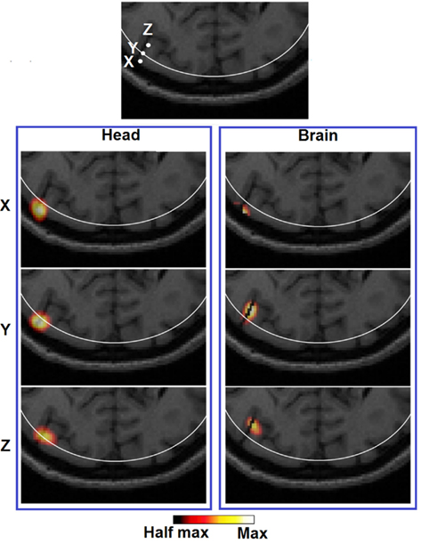
Figure 8. Images of three target perturbations located along the same cortical fold but different depth: 10.22 mm (X), 13.14 mm (Y), and 18.13 mm (Z), and the corresponding PSFs shown at FVHM using full head [column (Head)] and brain constrained [column (Brain)] reconstruction. The white contour on each MRI slice represents the 13 mm imaging depth.
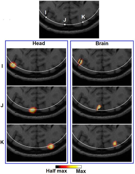
Figure 9. Images of three target perturbations located at different lateral positions but similar depth: 13.14 mm (I), 13.01 mm (J), and 13.07 mm (K), and the corresponding PSFs shown at FVHM using full head [column (Brain)] and brain constrained [column (Head)] reconstruction. The white contour on each MRI slice represents the 13 mm imaging depth.
In terms of imaging resolution, the use of “whole-brain” constraint for image recovery, a more homogenous (and less than 1000 mm3) LVHM spread provides the capability to distinguish between gyri as shown by activation X in Figure 8 (Brain), and between gyrus and sulcus as shown by activation Z in Figure 9 (Brain). Finally, the 3D cortical surface maps of localization error and LVHM in Figures 6 and 7 (Brain) also illustrate a much more homogeneous distribution of image accuracy and resolution throughout the FOV of the visual cortex as compared with Figures 6 and 7 (Head).
The quantitative results reported in this work (as obtained from a subject-specific anatomical head model with a chosen set of baseline tissue optical properties) will certainly vary by subject. Previous works suggest the variations on image quality due to different anatomies and tissue thickness (Heiskala et al., 2009b; Custo et al., 2010) and uncertainty in tissue optical properties (Heiskala et al., 2009a; Zhan et al., 2011) can be minimal when considering temporal imaging but there could exist abnormal variations in anatomy that cause the image quality to be affected significantly and this warrants further investigation in future studies. Additionally the effect of superficial physiology in the scalp may play a role in the results presented in this work, however, we have shown in previous studies that using appropriate functional data processing, it is possible to minimize their effects (White et al., 2009).
The work presented in this study, for conciseness, is limited to a single NIR wavelength and parameters relating to errors such as optode placements and variations to underlying optical properties are ignored. The choice of a using a specific wavelength (750 nm in the presented work) is appropriate, since most systems rely on specific wavelength measurements for the recovery of optical parameters and the methods and findings can easily be expanded for other wavelengths. Although the assumptions regarding the optode placements and underlying tissue optical properties are important when relating any findings to clinical applications, it is critically important to understand the underlying physical limits of optical parameters recovery when utilizing HD-DOT for neuroimaging studies.
Conclusion
Simulations have shown that HD-DOT methods that incorporate a head model which provides a realistic description of the spatial distribution of tissue optical properties are capable of imaging focal hemodynamic response up to 18 mm below an adult human scalp using whole-brain constrained reconstruction scheme within a 10 mm localization accuracy and resolution, which would allow the distinguish-ability of gyri. Yet further yield in imaging depth may be expected via the utility of more overlapping measurements, e.g., up to fourth and fifth nearest neighbors, as the dynamic range of future HD-DOT systems increase, or for subjects with less optically absorptive head tissues, e.g., neonates and young children.
The results presented herein provide the first comprehensive study evaluating the resolution and accuracy of HD-DOT with an anatomical head model and the use of a whole-brain constraint. It can serve as guidance on what image quality to expect throughout the cortical folds and approaches that might be taken to validate with fMRI. Admittedly the MRI-guided routine used in this study still relies on subject-specific MRIs to generate the forward head model. However recently studies which utilize a deformable atlas to construct subject-specific head model using various head surface geometry fitting schemes, have shown promise in both simulation (Heiskala et al., 2009b) and in vivo (Custo et al., 2010). Therefore a possible future work would be to evaluate the imaging performance for atlas-based HD-DOT methods.
Conflict of Interest Statement
The authors declare that the research was conducted in the absence of any commercial or financial relationships that could be construed as a potential conflict of interest.
Acknowledgments
This work has been funded by the National Institutes of Health (NIH) Grant R01EB009233-2.
References
Bevilacqua, F., Piguet, D., Marquet, P., Gross, J. D., Tromberg, B. J., and Depeursinge, C. (1999). In vivo local determination of tissue optical properties: applications to human brain. Appl. Opt. 38, 4939–4950.
Bluestone, A., Abdoulaev, G., Schmitz, C., Barbour, R., and Hielscher, A. (2001). Three-dimensional optical tomography of hemodynamics in the human head. Opt. Express 9, 272–286.
Boas, D. A., Chen, K., Grebert, D., and Franceschini, M. A. (2004a). Improving the diffuse optical imaging spatial resolution of the cerebral hemodynamic response to brain activation in humans. Opt. Lett. 29, 1506–1508.
Boas, D. A., Dale, A. M., and Franceschini, M. A. (2004b). Diffuse optical imaging of brain activation: approaches to optimizing image sensitivity, resolution, and accuracy. Neuroimage 23(Suppl. 1), S275–S288.
Boas, D. A., and Dale, A. M. (2005). Simulation study of magnetic resonance imaging-guided cortically constrained diffuse optical tomography of human brain function. Appl. Opt. 44, 1957–1968.
Brooksby, B., Jiang, S., Dehghani, H., Pogue, B. W., Paulsen, K. D., Weaver, J., Kogel, C., and Poplack, S. P. (2005). Combining near-infrared tomography and magnetic resonance imaging to study in vivo breast tissue: implementation of a Laplacian-type regularization to incorporate magnetic resonance structure. J. Biomed. Opt. 10, 051504.
Culver, J. P., Siegel, A. M., Stott, J. J., and Boas, D. A. (2003). Volumetric diffuse optical tomography of brain activity. Opt. Lett. 28, 2061–2063.
Custo, A., Boas, D. A., Tsuzuki, D., Dan, I., Mesquita, R., Fischl, B., Grimson, W. E., and Wells, W. III. (2010). Anatomical atlas-guided diffuse optical tomography of brain activation. Neuroimage 49, 561–567.
Custo, A., Wells, W. M. III, Barnett, A. H., Hillman, E. M., and Boas, D. A. (2006). Effective scattering coefficient of the cerebral spinal fluid in adult head models for diffuse optical imaging. Appl. Opt. 45, 4747–4755.
Dehghani, H., Eames, M. E., Yalavarthy, P. K., Davis, S. C., Srinivasan, S., Carpenter, C. M., Pogue, B. W., and Paulsen, K. D. (2008). Near infrared optical tomography using NIRFAST: algorithm for numerical model and image reconstruction. Commun. Numer. Methods Eng. 25, 711–732.
Dehghani, H., Srinivasan, S., Pogue, B. W., and Gibson, A. (2009a). Numerical modelling and image reconstruction in diffuse optical tomography. Philos. Transact. A Math. Phys. Eng. Sci. 367, 3073–3093.
Dehghani, H., White, B. R., Zeff, B. W., Tizzard, A., and Culver, J. P. (2009b). Depth sensitivity and image reconstruction analysis of dense imaging arrays for mapping brain function with diffuse optical tomography. Appl. Opt. 48, D137–D143.
Eggebrecht, A. T., White, B. R., Ferradal, S. L., Chen, C., Zhan, Y., Snyder, A. Z., Dehghani, H., and Culver, J. P. (2012). A quantitative spatial comparison of high-density diffuse optical tomography and fMRI cortical mapping. Neuroimage.
Gibson, A. P., Austin, T., Everdell, N. L., Schweiger, M., Arridge, S. R., Meek, J. H., Wyatt, J. S., Delpy, D. T., and Hebden, J. C. (2006). Three-dimensional whole-head optical tomography of passive motor evoked responses in the neonate. Neuroimage 30, 521–528.
Heiskala, J., Hiltunen, P., and Nissila, I. (2009a). Significance of background optical properties, time-resolved information and optode arrangement in diffuse optical imaging of term neonates. Phys. Med. Biol. 54, 535–554.
Heiskala, J., Pollari, M., Metsaranta, M., Grant, P. E., and Nissila, I. (2009b). Probabilistic atlas can improve reconstruction from optical imaging of the neonatal brain. Opt. Express 17, 14977–14992.
Koch, S. P., Habermehl, C., Mehnert, J., Schmitz, C. H., Holtze, S., Villringer, A., Steinbrink, J., and Obrig, H. (2010). High-resolution optical functional mapping of the human somatosensory cortex. Front Neuroenergetics 2:12.
Li, T., Gong, H., and Luo, Q. (2011). Visualization of light propagation in visible Chinese human head for functional near-infrared spectroscopy. J. Biomed. Opt. 16, 045001.
Niu, H., Khadka, S., Tian, F., Lin, Z. J., Lu, C., Zhu, C., and Liu, H. (2011). Resting-state functional connectivity assessed with two diffuse optical tomographic systems. J. Biomed. Opt. 16, 046006.
Obrig, H., and Villringer, A. (2003). Beyond the visible – imaging the human brain with light. J. Cereb. Blood Flow Metab. 23, 1–18.
O’Leary, M. A. (1996). Imaging with Diffuse Photon Density Waves. Ph.D. thesis, University of Pennsylvania, Philadelphia.
Pogue, B. W., Davis, S. C., Song, X., Brooksby, B. A., Dehghani, H., and Paulsen, K. D. (2006). Image analysis methods for diffuse optical tomography. J. Biomed. Opt. 11, 33001.
Strangman, G., Franceschini, M. A., and Boas, D. A. (2003). Factors affecting the accuracy of near-infrared spectroscopy concentration calculations for focal changes in oxygenation parameters. Neuroimage 18, 865–879.
White, B. R., and Culver, J. P. (2010a). Phase-encoded retinotopy as an evaluation of diffuse optical neuroimaging. Neuroimage 49, 568–577.
White, B. R., and Culver, J. P. (2010b). Quantitative evaluation of high-density diffuse optical tomography: in vivo resolution and mapping performance. J. Biomed. Opt. 15, 026006.
White, B. R., Snyder, A. Z., Cohen, A. L., Petersen, S. E., Raichle, M. E., Schlaggar, B. L., and Culver, J. P. (2009). Resting-state functional connectivity in the human brain revealed with diffuse optical tomography. Neuroimage 47, 148–156.
Keywords: tomography, functional monitoring and imaging, image reconstruction techniques
Citation: Zhan Y, Eggebrecht AT, Culver JP and Dehghani H (2012) Image quality analysis of high-density diffuse optical tomography incorporating a subject-specific head model. Front. Neuroenerg. 4:6. doi: 10.3389/fnene.2012.00006
Received: 19 March 2012; Accepted: 02 May 2012;
Published online: 24 May 2012.
Edited by:
Jean-Claude Baron, University of Cambridge, UKReviewed by:
David Boas, Massachusetts Institute of Technology, USAIlkka Nissilä, Aalto University, Finland
Copyright: © 2012 Zhan, Eggebrecht, Culver and Dehghani. This is an open-access article distributed under the terms of the Creative Commons Attribution Non Commercial License, which permits non-commercial use, distribution, and reproduction in other forums, provided the original authors and source are credited.
*Correspondence: Hamid Dehghani, School of Computer Science, University of Birmingham, Birmingham B15 2TT, UK. e-mail: h.dehghani@cs.bham.ac.uk