Information diversity in structure and dynamics of simulated neuronal networks
- 1 Department of Signal Processing, Tampere University of Technology, Tampere, Finland
- 2 Department of Mathematics, Tampere University of Technology, Tampere, Finland
Neuronal networks exhibit a wide diversity of structures, which contributes to the diversity of the dynamics therein. The presented work applies an information theoretic framework to simultaneously analyze structure and dynamics in neuronal networks. Information diversity within the structure and dynamics of a neuronal network is studied using the normalized compression distance. To describe the structure, a scheme for generating distance-dependent networks with identical in-degree distribution but variable strength of dependence on distance is presented. The resulting network structure classes possess differing path length and clustering coefficient distributions. In parallel, comparable realistic neuronal networks are generated with NETMORPH simulator and similar analysis is done on them. To describe the dynamics, network spike trains are simulated using different network structures and their bursting behaviors are analyzed. For the simulation of the network activity the Izhikevich model of spiking neurons is used together with the Tsodyks model of dynamical synapses. We show that the structure of the simulated neuronal networks affects the spontaneous bursting activity when measured with bursting frequency and a set of intraburst measures: the more locally connected networks produce more and longer bursts than the more random networks. The information diversity of the structure of a network is greatest in the most locally connected networks, smallest in random networks, and somewhere in between in the networks between order and disorder. As for the dynamics, the most locally connected networks and some of the in-between networks produce the most complex intraburst spike trains. The same result also holds for sparser of the two considered network densities in the case of full spike trains.
1 Introduction
Neuronal networks exhibit diverse structural organization, which has been demonstrated in studies of both neuronal microcircuits and large-scale connectivity (Frégnac et al., 2007; Voges et al., 2010; Sporns, 2011). Network structure, the connectivity pattern between elements contained in the network, constrains the interaction between these elements, and consequently, the overall dynamics of the system. The relationship between network structure and dynamics has been extensively considered in theoretical studies (Albert and Barabási, 2002; Newman, 2003; Boccaletti et al., 2006; Galas et al., 2010). In networks of neurons, the pattern of interneuronal connectivity is only one of the components that affect the overall network dynamics, together with the non-linear activity of individual neurons and synapses. Therefore, the constraints that structure imposes on dynamics in such systems are difficult to infer, and reliable methods to quantify this relationship are needed. Several previous studies employed cross-correlation in this context (Kriener et al., 2008; Ostojic et al., 2009), while the study reported in Soriano et al. (2008) proposed a method to infer structure from recorded activity by estimating the moment in network development when all of the neurons become fully connected into a giant component.
The structure and activity can be examined in a simplified but easily tractable neuronal system, namely in dissociated cultures of cortical neurons. Neurons placed in a culture have the capability to develop and self-organize into functional networks that exhibit spontaneous bursting behavior (Kriegstein and Dichter, 1983; Marom and Shahaf, 2002; Wagenaar et al., 2006). The structure of such networks can be manipulated by changing the physical characteristics of the environment where neurons live (Wheeler and Brewer, 2010), while the activity is recorded using multielectrode array chips. Networks of spiking neurons have been systematically analyzed in the literature (for example, see Brunel, 2000; Tuckwell, 2006; Kumar et al., 2008; Ostojic et al., 2009). In addition, models aiming to study neocortical cultures are presented in (Latham et al., 2000; Benayon et al., 2010), among others.
In this work, we follow the modeling approach of a recent study (Gritsun et al., 2010) in simulating the activity of a neuronal system. The model is composed of Izhikevich model neurons (Izhikevich, 2003) and the synapse model with short term dynamics (Tsodyks et al., 2000). We employ an information theoretic framework presented in Galas et al. (2010) in order to estimate the information diversity in both the structure and dynamics of simulated neuronal networks. This framework utilizes the normalized compression distance (NCD), which employs the approximation of Kolmogorov complexity (KC) to evaluate the difference in information content between a pair of data sequences. Both network dynamics in the form of spike trains and network structure described as a directed unweighted graph can be represented as binary sequences and analyzed using the NCD. KC is maximized for random sequences that cannot be compressed and small for the regular sequences with lot of repetitions. Contrary to KC, a complexity measure taking into account the context-dependence of data gives small values for the random and regular strings and is maximized for the strings that reflect both regularity and randomness, i.e., that correspond to the systems between order and disorder (Galas et al., 2010; Sporns, 2011). The notion of KC has been employed before to analyze experimentally recorded spike trains, i.e., the recordings of network dynamics, and to extract relevant features as in Amigó et al. (2004) and Christen et al. (2006). Another examples of application of information theoretic methods in the analysis of spike train data can be found in Paninski (2003).
The NCD has been used for analysis of Boolean networks in Nykter et al. (2008), where it demonstrated the capability to discriminate between different network dynamics, i.e., between critical, subcritical and supercritical networks. This study employs NCD in a more challenging context. As already mentioned, in neuronal networks the influence of structure on dynamics is not straightforwardly evident since both network elements (neurons) and connections between them (synapses) possess their own non-linear dynamics that contribute to the overall network dynamics in a non-trivial manner. The obtained results show that random and regular networks are separable by their NCD distributions, while the networks between order and disorder cover the continuum of values between the two extremes. The applied information theoretic framework is novel in the field of neuroscience, and introduces a measure of information diversity capable of assessing both structure and dynamics of neuronal networks.
2 Materials and Methods
2.1 Network Structure
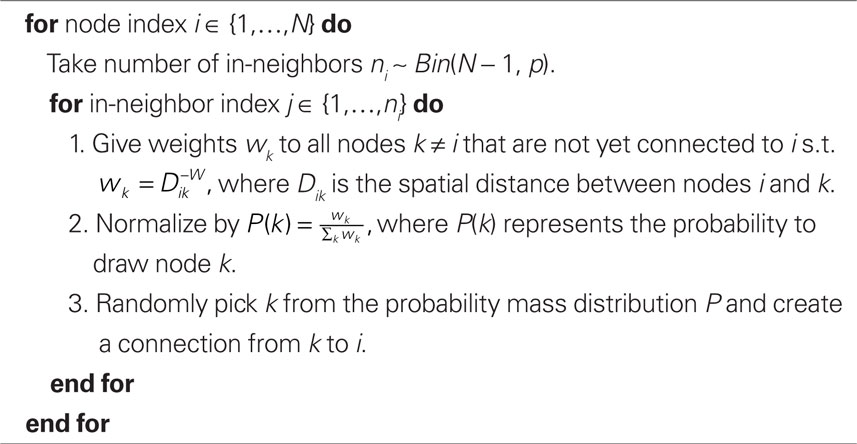
Different types of network structures are considered in this study. In locally connected networks (LCN) with regular structure every node is preferentially connected to its spatially closest neighbors. Only for high enough connectivity a node connects to more distant neighbors. In random Erdős–Rényi (RN) networks every pair of nodes is connected with equal probability regardless of their location. Finally, networks with partially local and partially random connectivity (PLCN) possess order and disorder in their structure. In Algorithm 1, we describe a unified scheme for generating these three types of networks.
Algorithm 1. Scheme for generating distance-dependent networks.
The scheme uses three parameters: probability of connection between a pair of nodes p ∈ [0,1], factor that defines dependence on distance W ≥ 0, and the spatial node-to-node distance matrix D ∈ ℝN × N. The matrix D is presumed positive and symmetric. For W = 0 the scheme results in a RN, as for W = ∞ we obtain a LCN. These latter networks are considered the limit cases of an arbitrarily big factor W: when choosing the in-neighbor one always picks the spatially closest one that has not yet been chosen as an in-neighbor. Randomness in the picking of the in-neighbors is applied only when there are two or more possible in-neighbors with the exact minimal distance from the considered node. In these cases, the in-neighbor is chosen by random.
It is notable that regardless of the choice of the distance-dependence factor W the scheme results in a network with in-degree distributed binomially as Bin(N−1, p). Equal in-degree distribution makes the considered networks comparable: each network has the same average number of neurons with a high number of synaptic inputs as well as those with a low number. This property does not arise in most studied models of networks with varying distance-dependence, as Watts–Strogatz networks (Watts and Strogatz, 1998) or Erdős–Rényi based models where the probability of connection is altered by the spatial distance between the nodes (see e.g., Itzhack and Louzoun, 2010).
2.1.1 NETMORPH: a neuronal morphology simulator
In addition to networks described above, we study biologically realistic neuronal networks. NETMORPH is a simulator that combines various models concerning neuronal growth (Koene et al., 2009). The simulator allows monitoring the evolution of the network from isolated cells with mere stubs of neurites into a dense neuronal network, moreover, observing the network structure determined by the synapses at given time instants in vitro. It simulates a given number of neurons that grow independently of each other, and forms synapses whenever an axon of a neuron and a dendrite of another neuron come near enough to each other. The neurite segments are static in the sense that when they are once put onto their places they are not allowed to move for the rest of the simulation.
The growth of the axons and dendrites is described by three processes: elongation, turning, and branching, all of which are only applied to the terminal segments of the dendritic and axonal trees. The elongation of a terminal segment obeys the equation

where vi is the elongation rate at time instant ti, v0 is the initial elongation rate, ni is the number of terminal segments in the arbor that the considered terminal segment belongs to, and F is a parameter that describes the dependence of the elongation rate on the size of the arbor.
The terminal segments continue to grow until a turning or branching occurs. The probability that a terminal segment j changes direction during time interval (ti, ti + Δt) obeys equation

where ΔLj(ti) is the total increase in the length of the terminal segment during the considered time interval and rL is a parameter that describes the frequency of turnings. The new direction of growth is obtained by adding perturbation to a weighted mean of previous growing directions. The most recent growing directions are given more weight than the earliest ones.
The probability that a terminal segment branches is given by

where ni is the number of terminal segments in the whole neuron at time ti and E is a parameter describing the dependence of branching probability on the number of terminal segments. Parameters B∞ and τ describe the overall branching probability and the dependence of branching probability on time, respectively – the bigger the constant τ, the longer the branching events will continue to occur. The variable γj is the order of the terminal segment j, i.e., how many segments there are between the terminal segment and the cell soma, and S is the parameter describing the effect of the order. Finally, the probability is normalized using the variable 
Whenever an axon and a dendrite of two separate neurons grow near enough to each other, there is a possibility of a synapse formation. The data consisting of information on the synapse formations, and hence describing the network connectivity, is output by the simulator. Technical information on the simulator and the model parameters that are used in this study are listed in Appendix 6.1.
2.1.2 Structural properties of a network
In this study we consider the network structure as a directed unweighted graph. These graphs can be represented by connectivity matrices M ∈ {0, 1}N × N, where Mij = 1 when there is an edge from node i to node j. The most crucial single measure characterizing the graphs is probably the degree of the graph, i.e., the average number of in- or out-connections of the nodes. When studying large networks, not only the average number but also the distributions of the number of in- and out-connections, i.e., in- and out-degree, are of interest.
Further considered measures of network structures are the shortest path length and the clustering coefficient (Newman, 2003). We choose these two standard measures in order to show differences in the average distance between the nodes and the overall degree of clustering in the network. The shortest path length lij (referred to as path length from now on) from node i to node j is the minimum number of edges that have to be traversed to get from i to j. The mean path length of the network is calculated as  where such path lengths lij where no path between the nodes exists are considered 0. The clustering coefficient ci of node i is defined as follows. Consider 𝒩i as the set of neighbors of node i, i.e., the nodes that share an edge with node i in at least one direction. The clustering coefficient of node i is the proportion of traversable triangular paths that start and end at node i to the maximal number of such paths. This maximal number corresponds to the case where the subnetwork 𝒩i ∪ {i} be fully connected. The clustering coefficient can thus be written as
As the connections to self (autapses) are prohibited, one can use the diagonal values of the third power of connectivity matrix M to rewrite Eq. 4 as
This definition of clustering coefficient is an extension of Eq. 5 in Newman (2003) to directed graphs. The clustering coefficient of the network is calculated as the average of those ci for which |𝒩i| > 1.
Examples of connectivity patterns of different network structure classes, including a network produced by NETMORPH, are illustrated in Figure 1. The figure shows connectivity of a single cell (upper row), the connectivity matrix in total with black dots representing the ones (middle row) and a zoomed in segment of the connectivity matrix (bottom row). The structure classes shown are a RN, three examples of PLCN obtained for different values of distance-dependence factor W, a LCN and a NETMORPH network. Connection probability p = 0.1 is used in all network types. Note the variability in the spread of neighbors within different networks: for RNs they are spread totally random, as for LCNs they are distributed around the considered neuron. Due to the boundary conditions the spread of the out-neighbors in LCN is not circular, as the nodes near the border have on average more distant in-neighbors than the ones located at the center. In NETMORPH networks the spread of the out-neighbors is largely dictated by the direction of the axonal growth.
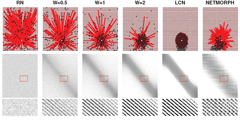
Figure 1. Upper: Examples of the connectivity patterns. White: target cell, red: cells having output to the target cell, black: cells receiving input from the target cell; Middle: Connectivity matrix. Y-axis: From-neuron index, X-axis: To-neuron index; Lower: Selected part of the connectivity matrix magnified.
2.2 Network Dynamics
2.2.1 Model
To study the network activity we follow the modeling approach presented in Gritsun et al. (2010). We implement the Izhikevich model (Izhikevich, 2003) of spiking neurons defined by the following membrane potential and recovery variable dynamics
and the resetting scheme
Parameters a, b, c, and d are model parameters and

is an input term consisting of both synaptic input from other modeled neurons and a Gaussian noise term. The synaptic input to neuron j is described by Tsodyks’ dynamical synapse model (Tsodyks et al., 2000) as

The parameter Aij accounts for the strength and sign (positive for excitatory, negative for inhibitory) of the synapse whose presynaptic cell is i and postsynaptic cell j – note the permutated roles of i and j compared to those in Tsodyks et al. (2000). The variable yij represents the fraction of synaptic resources in the active state and obeys the following dynamics:
Variables x and z are the fractions of synaptic resources in the recovered and inactive states, respectively, and τrec and τI are synaptic model parameters. The time instant tsp stands for a spike time of the presynaptic cell; the spike causes a fraction u of the recovered resources to become active. For excitatory synapses the fraction u is a constant U, as for inhibitory synapses the dynamics of the fraction u is described as

To solve the differential equations we apply Euler method on Eqs 6 and 7 and exact integration (see e.g., Rotter and Diesmann, 1999) on Eqs 10 and 11. The simulation setup for the activity model described above is discussed further in Section 3.1. Values of the model parameters and the initial conditions of the model are given in Appendix 6.2. Figure 2 illustrates a typical population spike train of different network classes with connection probability 0.1, and a magnified view of one of their bursts.
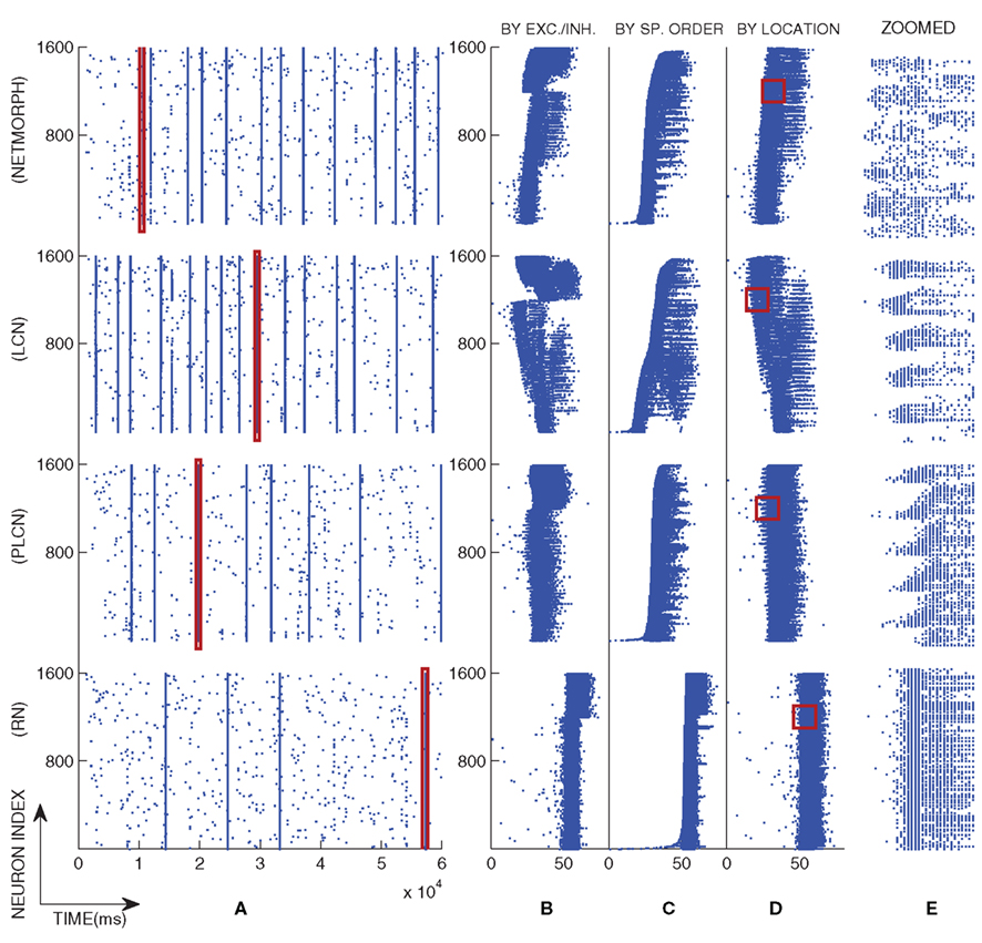
Figure 2. An example of population spike trains of four different networks with a selected burst magnified. The distance-dependence factor W = 1 is used in the PLCN network. (A): The full population spike train, (B–D): The spiking pattern of the selected burst illustrated by different orderings of the neurons, and (E): The selected region in (D) magnified. In (B) the neurons are primarily ordered by their type and secondarily by their location in the grid such that the lower spike trains represent the excitatory neurons and the upper spike trains the inhibitory neurons. In (C) the neurons are ordered by the time of their first spike in the selected burst, i.e., the lower the spike train is, the earlier its first spike occurred. In (D) the neurons are ordered purely by their location in the grid.
2.2.2 Synchronicity analysis
Given a population spike train, we follow the network burst detection procedure as presented in Chiappalone et al. (2006), but using a minimum spike count minSpikes = 400 and maximal interspike interval ISI = 10 ms. Once the starting and ending time of the burst are identified, the spike train data of the burst are smoothed using a Gaussian window with deviation 2.5 ms to obtain a continuous curve as shown in Figure 3. The shape of the burst can be assessed with three statistics that are based on this curve: the maximum firing rate (mFr), half-width of the rising slope (Rs) and half-width of the falling slope (Fs) (Gritsun et al., 2010).
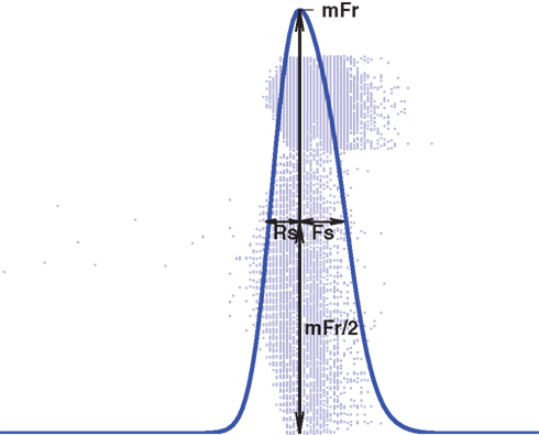
Figure 3. Illustration of the meaning of variables mFr, Rs, and Fs. (as defined in Gritsun et al., 2010).
In addition to the network burst analysis, we estimate the cross-correlations between spike trains of two neurons belonging to the same network. We follow the method presented in Shadlen and Newsome (1998), where the cross-correlation coefficient (CC) between spike trains of neurons j and k is defined as  Here, the variable Ajk represents the area below the cross-correlogram and is computed as
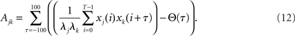
The variable xj(i) is 1 for presence and 0 for absence of a spike in the ith time bin of spike train of neuron j, λj is the mean value of xj(i) averaged over i, and T is the number of time bins in total. The running variable τ is the time lag between the two compared signals, and the weighting function Θ is chosen triangular as Θ(τ) = T−|τ|.
2.3 Information Diversity as a Measure of Data Complexity
Complexity of different types of data and systems has been studied in numerous scientific disciplines, but no standard measure for it has been agreed upon. The most widely used measures are probably Shannon information (entropy) and the theoretical KC. Shannon information measures the information of a distribution. Thus, it is based on the underlying distribution of the observed random variable realizations. Unlike Shannon information, KC is not based on statistical properties, but on the information content of the object itself (Li and Vitanyi, 1997). Hence, KC can be defined without considering the origin of an object. This makes it more attractive for the proposed studies as we can consider the information in individual network structures and their dynamics. The KC C(x) of a finite object x is defined as the length of the shortest binary program that with no input outputs x on a universal computer. Thereby, it is the minimum amount of information that is needed in order to generate x. Unfortunately, in practice this quantity is not computable (Li and Vitanyi, 1997). While the computation of KC is not possible an upper bound can be estimated using lossless compression. We utilize this approach to obtain approximations for KC.
In this work we study the complexity of an object by the means of diversity of the information it carries. The object of our research is the structure of a neuronal network and the dynamics it produces. There are numerous existing measures for the complexity of a network (Neel and Orrison, 2006), and a few measures exist also for the complexity of the output of a neuronal network (Rapp et al., 1994), but no measure of complexity that could be used for both structure and dynamics has – to the best of our knowledge – been studied. To study the complexity of the structure we consider the connectivity matrix that represents the network, as for the complexity of the network activity we study the spike trains representing spontaneous activity in the neuronal network. We apply the same measure for assessing complexity in both structure and dynamics.
2.3.1 Inferring complexity from NCD distribution
We use the NCD presented in Li et al. (2004) as a measure of information distance between two arbitrary strings. The NCD is a computable approximation of an information distance based on KC. The NCD between strings x and y is defined by
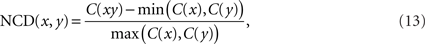
where C(x) and C(y) are the lengths of the strings x and y when compressed – accounting for approximations of KCs of the respective strings – and C(xy) is that of the concatenation of strings x and y. In our study we use standard lossless compression algorithms for data compression1.
The NCD has recently been used in addressing the question whether a set of data is similarly complex as another (Emmert-Streib and Scalas, 2010), based on a statistical approach. In another study (Galas et al., 2010), the complexity of a set of strings is estimated using a notion of context-dependence, also assessable by the means of the NCD. We follow the latter framework and aim at estimating the complexity of an independent set of data – in our study, this set of data is either a set of connectivity patterns or a set of spike trains. In Galas et al. (2010) the set complexity measure is introduced; it can be formulated as

To calculate the set complexity Ψ one has to approximate the KCs of all strings xi in the set S = {x1,…,xN} and the NCDs dij = NCD(xi,xj) between the strings. The functions f and g of NCD values are continuous on interval [0,1] such that f reaches zero at 1 and g reaches zero at 0.
In this study we, for reasons to follow, diverge from this definition. We define the complexity of a set of data as the magnitude of variation of NCD between its elements: the wider the spread of NCD values, the more versatile the set is considered. That is, a complex set is thought to include both pairs of elements that are close to each other from an information distance point of view, pairs of elements that are far from each other, and pairs whose distance is somewhere in between.
Although the variation of NCD by no means captures all the properties that are required of a complexity measure and fulfilled by the set complexity Ψ, it lacks the difficulty arising in determining the functions f and g in Eq. 14. Let us consider this in more detail from the point of view that we do not know how the functions f and g should be like – which is a fact, apart from the knowledge on them having roots in 0 and 1. Suppose we have two finite sets of strings, 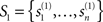 and
and 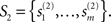 Denote the NCDs between the strings of set S1 by
  where i,j ∈ {1,…,n}, and accordingly, let
  be the NCDs between the strings of set S2. If any of the NCDs
  (i≠j) is unique in the sense that it is unequal to all NCDs
  (k≠l), then we find an ε-neighborhood
  that contains an NCD value of S1 but none of those of S2. Thereby, we can choose the functions f and g such that the value of f × g is arbitrarily large at
  and arbitrarily small outside
  leading to Ψ(S1) > Ψ(S2). We can generalize this to a case of any finite number of sets S1,…,SN: if for set SI, I ∈ {1,…,N} there is an NCD value
  (i ≠ j) that is unequal to all other NCD values
  (J ≠ I, k ≠ l), then the functions f and g can be configured such that ∀J ≠ I:Ψ(SI) > Ψ(SJ). Hence, the lack of knowledge on functions f and g imposes severe restrictions on the eligibility of the set complexity Ψ as such.
What is incommon for the proposals for f and g presented in Galas et al. (2010) is that the product function f × g forms only one peak in the domain [0,1]. The crucial question is: where should this peak be located – ultimately, this is the same as asking: where is the boundary between “random” and “ordered” sets of data? Adopting the wideness of NCD distribution as a measure of data complexity is a way to bypass this problem. The wider the spread of NCD values, the more likely it is that some of the NCD values produce large values for f × g. Yet, difficulties arise when deciding a rigorous meaning for the “wideness” or “magnitude of variation” of the NCD distribution. In the present work, the calculated NCD distributions are seemingly unimodal; thereby we use the standard deviation of the NCD distribution as the measure of complexity of the set.
2.3.2 Data representation for complexity analysis
Two different data analysis approaches to studying the complexity are possible (Emmert-Streib and Scalas, 2010): one can assess (1) the complexity of the process that produces a data realization, or (2) the complexity of the data realization itself. In this study we will apply the approach (2) in both estimating the complexity of structure and the complexity of dynamics. To study the complexity in the context-dependent manner described in Section 2.3.1 we divide the data into a set of data, and represent it as a set of strings. For the structure, the rows of the connectivity matrix are read to strings, i.e., each string s shows the out-connection pattern of the corresponding neuron with si = “0” if there is no output to neuron i and si = “1” if there is one. The NCDs are approximated between these strings. In order to compute the NCD of the dynamics every spike train is converted into a binary sequence. Each discrete time step is assigned with one if a spike is present in that time slot, and with zero otherwise. For example, a string “0000000000100101000” would correspond to a case where a neuron is at first silent, then spikes at time intervals around 10Δt, 13Δt and 15Δt, where Δt is a sampling interval. For the compression of strings we use the general purpose data compression algorithm 7zip2. The compressor parameters and the motivation for this particular compression method are given in Appendix 6.3.
3 Results
3.1 Simulation Setup
In the present paper we study both structural and dynamical properties of networks of N = 1600 neurons. Regarding the choice of the structure of neuronal networks we base our approach on the growth properties of those networks produced by the NETMORPH simulator. To choose a trade-off between biological reality and ease of comparison to other types of networks we set the initial cell positions in a two-dimensional regular 40 × 40 grid. The present work does not consider continuous boundaries, i.e., the physical distance between the neurons is the standard Euclidean distance. The distance between adjacent neurons is set ≈25 μm, which is chosen such that the density of neurons corresponds to one of the culture densities examined in Wagenaar et al. (2006) (1600 cells/mm2). Figure 4 shows the average connection probability in a NETMORPH network as a function of time, where the average is taken over 16 simulation realizations. The standard deviation of the connection probability is found very small between different realizations (<0.002), hence only mean values are plotted here.
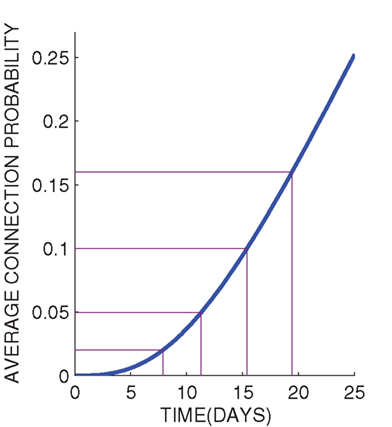
Figure 4. Connection probability as a function of time in the structure of networks generated by the NETMORPH simulator.
The main emphasis throughout this article will be on connection probabilities p = 0.02, 0.05, 0.1, 0.16 that, according to Figure 4, correspond to days 8, 11, 15, and 19 in vitro. The selected range of days in vitro is commonly considered in experimental studies of neuronal cultures. The connection probabilities 0.1 and 0.16 of 15th and 19th DIV, respectively, are in accordance with experimental studies that consider the connectivity of a mature network to be 10–30% (Marom and Shahaf, 2002).
Other considered networks are generated by Algorithm 1 using the abovementioned connection probabilities. The distance-dependence factors for these networks are chosen as W = 0, 0.5, 1, 2, 4, 10, ∞.
The spiking activity in the abovementioned networks is studied by simulating the time series of the N = 1600 individual neurons according to Section 2.2. The connectivity matrix of the modeled network defines which synaptic variables yij need to be modeled: the synaptic weights Aij are non-zero only for non-zero connectivity matrix entries Mij, hence for such (i,j) that Mij = 0 the synaptic variables yij can be ignored in terms of Eq. 9. In this article we disallow multiple synapses from a neuron to another. Throughout the paper the fraction of the inhibitory neurons is fixed to 25%, which are picked by random, and the sampling interval is fixed to 0.5 ms.
3.2 Network Structure Classes Differ in Their Graph Theoretic Properties
We first study the structural properties of the network classes presented above by the means of measures introduced in Section 2.1.2. The in-degree distributions of the networks generated by Algorithm 1 are always binomial, as the out-degree distributions vary. Empirically calculated out-degree distributions, path length distributions, and local clustering coefficient distributions are shown in Figure 5, together with the respective NETMORPH distributions.
Figure 5. Out-degree, path length and clustering coefficient distributions plotted for different network classes and different connection probabilities. The power coefficient W = 1 is used for PLCN networks. The mean path lengths and mean clustering coefficients are shown in association with the respective curves.
One can observe an increase in the mean path length as well as mean clustering coefficient with the increase of distance-dependence factor W, i.e., when moving from RN toward LCN. The out-degree distributions of NETMORPH networks are wider than those of any other type of network, but regarding the width and mean of the path length and clustering coefficient distributions the NETMORPH networks are always somewhere between RN and LCN.
3.3 Networks with Different Structure Show Variation in Bursting Behavior
For the activity part we simulate 61 s of spike train recordings using the models described in Section 2.2 and the model parameters described in Appendix 6.2. In all of our simulations a network burst occurs in the very beginning due to the transition into a steady state, which is why we ignore the first second of simulation. We simulate a set of spike trains for structure classes W = 0, 1, ∞ and NETMORPH using connection probabilities p = 0.02, 0.05, 0.1, 0.16. The average connection weight and other model parameters stay constant, only the connectivity matrix varies between different structure classes and different connection probabilities. In the case of p = 0.02 none of the networks shows bursting behavior, for p = 0.05 a burst emerges in about one out of three 1-min simulations, as for p = 0.1 and p = 0.16 there are bursts in every 1-min recording. Table 1 shows the acquired mean bursting frequencies – they are comparable to the ones obtained in Gritsun et al. (2010). We concentrate on the two bigger connection probabilities.
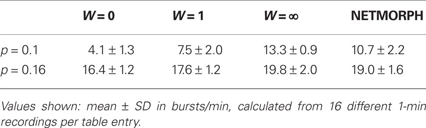
Table 1. Bursting rates of networks of different structure classes.
The difference between the intraburst patterns of the different networks can already be observed in the magnified burst images in Figure 2, particularly in 2C where the effect of the location of the neuron in the grid is neglected. We show the difference by studying the following burst statistics: spike count per burst (SC), and the three burst shape statistics defined above (mFr, Rs, and Fs). Figure 6 shows the distribution of these statistics in activity simulations of different network structure classes. The means as well as the medians of the three latter measures for both the NETMORPH and W = 1 networks constantly fall between the two extremes, LCN and RN. The same does not hold for SC.
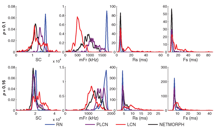
Figure 6. Distributions of spike count/burst (SC, far left), maximum firing rate in a burst (mFr, middle-left), rising slope length (Rs, middle-right), and falling slope length (Fs, far right) for spike trains obtained by using different structure classes and different connection probabilities (upper: 0. 1; lower: 0.16). The distance-dependence factor W = 1 is used for PLCN. Histograms are smoothed using a Gaussian window with standard deviation = range of values/100.
We test the difference of the medians statistically between different structure classes using U-test. The null hypothesis is that the medians of two considered distributions in a panel of Figure 6 are equal. The distributions of each measure (SC, mFr, Rs, Fs) and each network density are tested pairwise between the different network types. The test shows similarity of medians of Rs distributions between NETMORPH network and PLCN with connection probability 0.1 (p-value = 0.59), but not in the case of connection probability 0.16 (p-value = 1.7 × 10⁻¹³). The same holds for medians of Fs distributions of these networks, respective p-values being 0.20 and 0.0027. In all the rest of the cases the null hypothesis of medians of any measure being the same between any two distributions of different structure classes can be rejected, as none of the p-values exceeds 0.002. The variances of the distributions are not tested, but one can observe that LCNs clearly produce the widest SC, Rs, and Fs distributions.
3.4 Complexity Results in Structure and Dynamics
We start by studying simultaneously the KC of the rows of a connectivity matrix and the KC of the spike trains of the corresponding neurons. We generate a network for each structure class (W = 0, 0.5, 1, 2, 4, 10, ∞; NETMORPH) and a population spike train recording for each of these networks. A set of 80 neurons is randomly picked from the N = 1600 neurons retaining the proportion of excitatory and inhibitory neurons. This data set is considered representative of the whole set of neurons. Figure 7 shows approximations of KCs for both structure and dynamics of different structure classes and different connection probabilities. The value of C(struc) shows the length of a compressed row of the connectivity matrix as C(dyn) is the length of the compressed spike train data of the corresponding neuron.
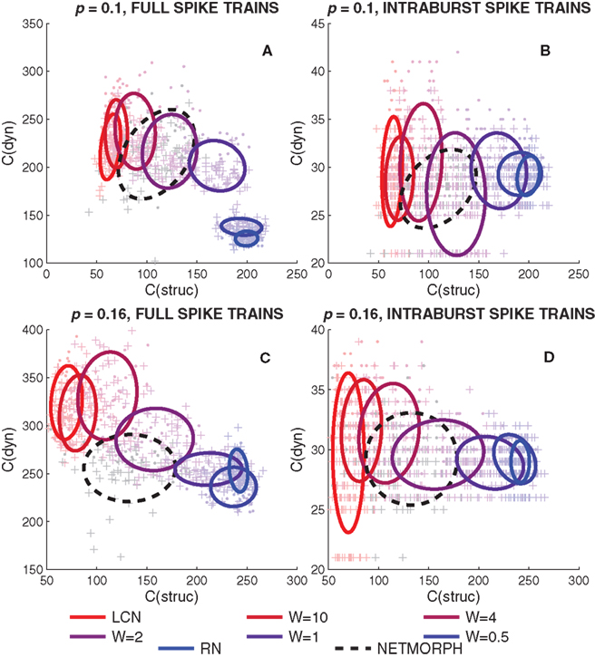
Figure 7. Kolmogorov complexity approximation of a spike train of a neuron (dyn) versus the KC approximation of the respective row of connectivity matrix (struc). (A,C): The full spike train of a neuron read into the string to be compressed. (B,D): Intraburst segments of the spike train read into separate strings (i.e., several “C(dyn)”-values possible for each “C(struc)”-value). In (A,B) the connection probability of the networks is 0.1, in (B,D) 0.16. The markers “+” represent excitatory neurons, as “·” are inhibitory. The ellipses drawn represent 67% of the probability mass of a Gaussian distribution with the same mean and covariance matrix as the plotted data.
Figure 7 shows that the mean of the compression lengths of full spike train data descends when moving from local to random networks, as the mean compression length of columns of connectivity matrix ascends. The rising of the C(struc) is in accord with the fact that random strings maximize the KC of a string, whereas the descending of the mean values of C(dyn) can be explained by the decrease in the number of bursts. A slightly similar trend is visible when studying the KC of intraburst spike trains, but more than that, the range of values of C(dyn) seems to decrease when moving from local to random networks.
However, as pointed out earlier, the KC alone does not tell much about diversity of the data set, only the information content of each element of the set alone. We wish to address the question of to what extent the information in one element is repeated or near-to-repeated in the other elements. We first analyze the structure and dynamics data using alternative measures, namely, Hamming distance (HD) and cross-correlation coefficient (CC). HD counts the proportion of differing bits in two binary sequences: it equals zero for identical sequences and one for sequences that are inverse of each other. The same elements as those in Figures 7A,C are analyzed using HD, i.e., the rows of connectivity matrix and spike trains of the corresponding neurons. The same number of 80 sample neurons is picked randomly, and HD is computed between the  pairs of neurons. In addition, the dynamics is analyzed using CC between pairs of spike trains. The CC measures similarity between two spike trains and is capable of capturing time shifts between the signals. Hence the CC serves as an extension of the HD, or of the inverse of HD (as cross-correlation measures similarity and HD measures divergence). Figure 8 shows the distribution of HD computed for both structure and dynamics (Figures 8A,C) and that of CC computed for dynamics versus HD computed for structure (Figures 8B,D).
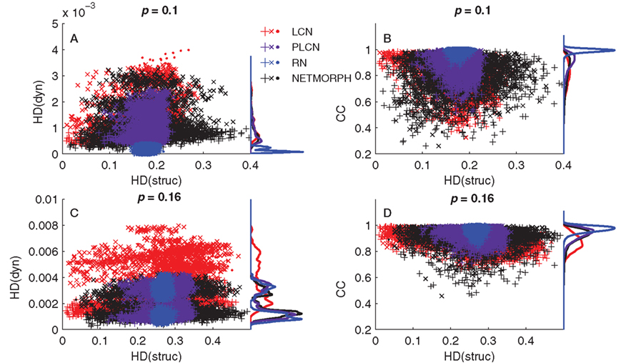
Figure 8. (A,C): Hamming distances between spike trains (dyn) versus the HD between the corresponding rows of connectivity matrix (struc). (B,D): Cross-correlation coefficient between spike trains (CC) versus the HD between the corresponding rows of connectivity matrix. In all panels the markers “+” represent comparisons of two excitatory neurons, “x” are comparisons between excitatory and inhibitory neurons, and “·” are comparisons between two inhibitory neurons. The distance-dependence factor W = 1 is used for the PLCN.
In Figures 8A,C one can observe the widening of the HD distribution in both structure and dynamics when moving from random to local networks. The same applies for the CC distribution (Figures 8B,D). The HD(struc) distributions of the most locally connected networks are wider than that of RN, because for each neuron there exist some neurons with a lot of common out-neighbors (the spatially nearby neurons, small HD value) and some neurons with zero or near to zero common out-neighbors (the spatially distant neurons, large HD value). For some of the considered networks a bimodal distribution of HD(dyn) can be observed. In such cases, the peak closer to zero corresponds to the comparison of neurons of the same type (excitatory–excitatory or inhibitory–inhibitory), while the peak further from zero corresponds to comparison of neurons of different type (excitatory–inhibitory). This bimodality is due to the difference in intraburst patterns between excitatory and inhibitory neurons: Figure 2B shows that on average the inhibitory population starts and ends bursting later than the excitatory one. This effect is most visible in RNs, as can be observed both in Figures 2 and 8A. As for the CCs, the distributions are unimodal. This indicates that the differences between the spiking patterns of inhibitory and excitatory neurons are observable on small time scale (HD uses the bins of width 0.5 ms), but not on large time scale (cross-correlations are integrated over an interval of ±50 ms). This is further supported by the fact that when the time window for CC calculations is narrowed, the CCs between neurons of same type become distinguishable from those between neurons of different type (data not shown).
Both HD and cross-correlation, however, assess the similarity between the data by observing only local differences. The HD determines the average difference between the data by comparing the data at exact same locations, as the cross-correlation allows some variation on the time scale. Both measures fail to capture similarities in the data if the similar patterns in the two considered data sequences lie too far from each other. This is also the case if the sequences include more subtle similarities than time shifts, e.g., if one sequence is a miscellaneous combination of the other’s subsequences. Thereby, we proceed to the information diversity framework presented in Section 2.3.1. We take the same elements as in Figure 7 – rows of connectivity matrix and full spike train data of neurons or intraburst segments only – and calculate the NCDs between these elements. These NCD distributions are plotted in Figure 9.
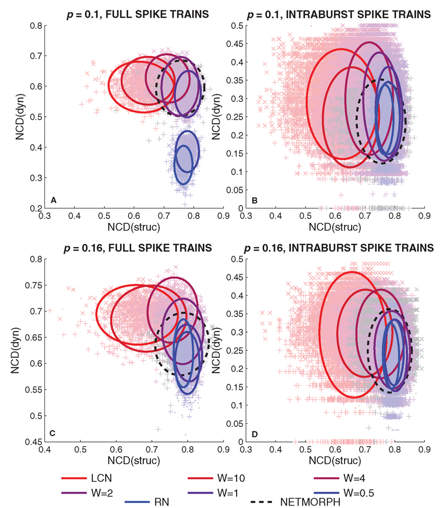
Figure 9. Normalized compression distances between spike trains of neurons (dyn) versus the NCD between respective rows of connectivity matrix (struc). The four figures arranged in a similar manner as in Figure 7, i.e., in (A,C) full spike trains are considered, and in (B,D) intraburst spike trains are considered. The ellipses drawn represent 90% of the probability mass of a Gaussian distribution with same mean and covariance matrix as the plotted data.
One can observe a gradual increase in the mean values of NCD(struc) with the increase of randomness to the structure of the network in Figure 9. This is rather expected: the more randomness applied to the structure of the network, the further away the connectivity data of different neurons are from each other. As for the NCD(dyn) values between full spike train data of neurons, one can observe a gradual decrease in the mean value with the increase of randomness, and a slightly similar evolution is visible in the burst-wise calculations as well. Both this and the decrease in the deviation of the NCD(dyn) values are in accordance with the properties of intraburst spike patterns illustrated in Figure 2: the spike train data seem more diverse and wider-spread in the local networks than in the random ones. Furthermore, as the bursting frequency is higher in LCNs than in RNs (Table 1), the analyzed LCN spike trains (1 min recordings) show more variability than those of RN. Consequently, the mean NCD(dyn) is visibly higher in LCN. When analyzing the dynamics of the intraburst interval, data variability is less pronounced and the difference between the means of NCD(dyn) distributions is smaller.
We repeat the experiment of Figure 9 10 times, and for each entry we calculate the standard deviations of NCD distributions (i.e., the complexities in our definition) of both structure and dynamics. Table 2 shows the mean complexities and their standard deviations, and the network classes in which the complexity is significantly different from that of a RN. The table shows that the structural complexity decreases with the increase of randomness to the structure. The complexity of full spike trains shows a less consistent trend. For sparser networks (p = 0.1), the more locally connected networks produce more complex full spike trains than RNs, as for denser networks (p = 0.16), only one of the PLCNs has statistically different complexity from that of RNs. We consider the latter statistical difference an outlier as a clear trend is absent. For the intraburst complexities the results suggest that the LCNs together with NETMORPH and some of the most locally connected PLCNs produce more complex dynamics than RNs.
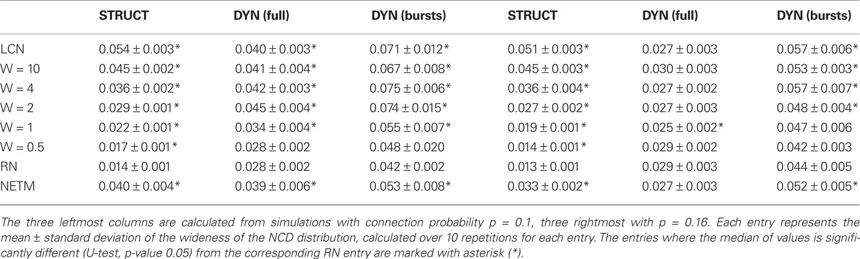
Table 2. Complexities calculated as standard deviations of NCD distributions for both elements of structure and dynamics.
The information diversity results of Table 2 do not clearly indicate which network produces the most complex dynamics. The p-values for the test whether the information diversity of the most complex full spike trains is different from that of the second most complex are 0.13 and 0.38 for sparse and dense networks, respectively. For the intraburst complexities the respective p-values are 0.80 and 0.62. The results for the complexity of structure are qualitatively the same when considering the columns of connectivity matrix, i.e., the in-connection patterns, instead of rows (data not shown). Furthermore, the decrease in the complexity of the structure by the increase in randomness is also present in the case where the neurons in the connectivity matrix are randomly permutated. This shows that the trend in the structural complexity in Table 2 is not an artifact of the order in which the neuron connectivities are read into strings.
3.5 Conclusion
The structure of RNs are described by low path length and low clustering coefficient, and further by high KC and low information diversity. The RN dynamics is described by short and relatively rare bursts, and hence low KC of the spike train data. As the opposite, the structure of LCNs show longer path length and greater clustering coefficient, and the KC approximations of the structural data are small while the information diversity is large. The bursts in the LCN spike trains are longer and more frequent than in RN spike trains. The KC approximations of the LCN spike train data are large on average. Based on the variation in NCD, the intraburst complexity is higher in LCN output than in that of RN, and for the sparser of the two network densities the same holds for complexities of full spike trains.
The in-between networks, PLCNs, fall between the two extremes (RN and LCN) by their structural properties as well as their bursting behavior. The same holds for the biologically realistic NETMORPH networks. The information diversity of the structure of these networks is between that of RN and LCN. Similarly to LCNs, the intraburst dynamics of NETMORPH networks as well as the most locally connected PLCNs are more complex in terms of NCD variation than that of RNs.
4 Discussion
In this work we present and apply an information diversity measure for assessing complexity in both structure and dynamics. According to this measure the neuronal networks with random structure produce less diverse spontaneous activity than networks where the connectivity of neurons is more dependent on distance. The presented study focuses on only one neuronal activity model, i.e., Izhikevich type neurons with dynamical model of synapses (Tsodyks model), and the networks of fixed size (N = 1600). The further studies testing alternative models and examining the influence of network size are needed to confirm these findings. Still, the presented results demonstrate capability of the employed measure to discriminate between different network types.
The basis for the present study is the question: if one changes the structure of the neuronal network but keeps the average degree (or even the whole in-degree distribution) constant, how does the spontaneous activity change? In the activity simulations, all model parameters remain constant, only the connectivity matrix is changed between the simulations of different network types; hence the variation in bursting properties emerges from the structure of the network only. The selected algorithm for generation of network structure possesses the capability to tune distance-dependence on a continuous scale. As a result, we have not only fully locally connected networks, where a neuron always first connects to its nearest spatial neighbors before the distant ones (W = ∞, i.e., LCN), and fully random networks (W = 0, i.e., RN), but everything in between (0 < W < ∞, PLCN). The RNs correspond to directed Erdős–Rényi networks that are widely used in similar studies in the field. These networks are characterized by a binomial degree distribution; hence the choice of binomial in-degree distribution for all network types. The only network class to violate this binomiality are the NETMORPH networks, which are considered in order to increase the biological plausibility of the study. The results showing that the NETMORPH networks are placed somewhere between the LCNs and RNs by most of their structural and dynamical properties also support the use of Algorithm 1 for the network generation. If this was not the case, one would have to try to find another way to produce networks with as extreme properties as those in NETMORPH networks. The range of networks between LCN and RN could also be produced with an application of Watts–Strogatz’ algorithm (Watts and Strogatz, 1998). The crucial difference is that in our in-between networks (PLCNs) the “long-range connections” are the shorter the bigger the parameter W is, while in Watts–Strogatz’ model the long-range connections are (roughly) on average equally long in all in-between networks. By a long-range connection we mean any connection to neuron A from neuron B when A is not yet connected to all neurons that are spatially nearer than B.
The complexity framework presented in this paper is adopted from Nykter et al. (2008), where critical Boolean networks are found to have the most complex dynamics out of a set of various Boolean networks. The method for estimating the complexity in the present work is different in the way that we apply the NCD measure between elements of a set that represents the object whose complexity is to be estimated (connectivity matrix, population spike train), not between different output realizations as in Nykter et al. (2008). This allows the estimation of the complexity of the object itself, not of the set of objects generated with the same process. The complexity of the object is assessed by the diversity of the information it carries. Although technically applicable to any set of strings, this is not supposed to be a universal measure of complexity. However, its use lacks the difficulties that arise when applying an alternative set complexity measure defined in Galas et al. (2010), as discussed in Section 2.3.1. The said non-universality of our measure stems from the limited range of deviation values that a NCD distribution can have, and on the other hand, the plain standard deviation might not be a good measure of wideness if the underlying distributions were multimodal. In this work all studied NCD distributions are unimodal. Furthermore, we only apply this complexity measure on data of comparable lengths and comparable characteristics, hence the resulting complexities are also comparable to each other. This may not be true in the opposite case, for example, spike trains of length 1 s and 1 h cannot be compared in an unbiased way.
In this study we show how the NCD values of both structure and dynamics of a neuronal network are distributed across the [0,1] × [0,1]-plane in the model networks (Figure 9), and calculate the mean information diversities of both structure and dynamics (Table 2). The Figures 9A,C themselves give a good overview of the interplay between structural and dynamical information diversity. They show that the NCD distributions, computed for the considered types of networks, follow a visible trajectory. This trajectory is not evident when observing the widths of the NCD distributions only, nor when computing simpler distance measures (e.g., HD). The trajectory follows an “L”-shape, which is slightly violated by the NETMORPH NCD distribution (see Figure 9C). Whether there exists a network of the same degree that would span the whole “L”-shaped domain or a “superdiverse” network whose NCD values would cover also the unoccupied corner of the “L”-rectangle remains an open question. We have shown that such networks do not exist among the model classes studied here, and in the light of the results shown we also doubt the existence of such networks altogether, given the constraints of binomial in-degree distribution and the selected connection probability.
The different networks are separable also by the KC approximations of their structure and dynamics (Figure 7). However, we consider the KC analysis alone insufficient because it lacks the notion of context-dependence: the KC of a spike train would be maximized when the on-set of neurons (i.e., spikes) are as frequent as off-set of neurons (i.e., silent time steps) and randomly distributed in time. The effect of number of spikes on KC is already seen in Figures 7A,C: the KCs of spike trains of dense networks, where the number of spikes is greater, are on average greater than those of sparse networks. This is contrary to the case of context-dependent complexities, as shown in Table 2, where the information diversities of full spike trains of dense networks are on average smaller than those of sparse networks. This leads to a profound question: how much spiking and bursting can there be before the activity is too random in order to contain any usable information? We believe that in order to address this question one has to apply a context-dependent measure of complexity instead of KC.
The complexity result in Table 2 concerning the information diversity of structure seems to contradict with the general notion according to which the most regular structure should be less complex than the structure that possesses both regularity and randomness (Sporns, 2011). It should be noted, however, that also the most regular networks studied in this work (LCNs) occupy a degree of randomness, since their in-degree distribution is binomial and since farthest neighbors of a neuron are picked by random out of all equally distant ones. There is a multitude of possibilities for the most ordered structure, other than the one chosen in this work. For example, in Sporns (2011) a fully connected network is suggested to be a highly ordered neuronal system. Applying the information diversity measure to such structure in the framework of Table 2 gives a structural complexity of ≈0.0268, which is less than that of the majority of the studied PLCNs. Hence, we regard the proposed measure eligible to assess the complexity of the structure.
In addition to analysis of well defined models, the presented measure can be used for analysis of experimental data. The method is straightforwardly applicable to neuronal activity recorded in the form of spike trains. Conversion of spike trains into binary sequences is described in the method section of this paper, as well as in the previous studies (Christen et al., 2006; Benayon et al., 2010). It can be observed that variability in NCD distribution corresponds to the variability in spiking patterns within population bursts. Similar measures of entropy and KC have been applied before, but the capability of the NCD to capture context between different data makes it suitable for assessing data complexity. The presented measure can be used to analyze different phases in neuronal network growth, where the structure is simulated by publicly available growth simulators (Koene et al., 2009; Acimovic et al., 2011). Analysis of network structure, using the procedure described in this paper, can be employed for this study. Analysis of the structure and dynamics of the presented models can be used in relation to the in vitro studies with modulated network structure. The results of model analysis can help to predict and understand the recorded activity obtained for certain network structures imposed by the experimenter (Wheeler and Brewer, 2010). Finally, the NCD variation as a measure of structural complexity, can be applied to analyze the large-scale functional connectivity of brain networks, similarly to the examples pointed in Sporns (2011).
The framework proposed in this study provides a measure of data complexity that is applicable to both structure and dynamics of neuronal networks. According to this measure, the neuronal networks with random structure show consistently less diverse intraburst dynamics than the more locally connected ones. The future work will incorporate a larger spectrum of different network structures in order to discover the extreme cases that more clearly maximize or minimize the complexity of dynamics.
Conflict of Interest Statement
The authors declare that the research was conducted in the absence of any commercial or financial relationships that could be construed as a potential conflict of interest.
5 Acknowledgments
The authors would like to acknowledge the following funding: TISE graduate school, Academy of Finland project grants no. 106030, no. 124615, and no. 132877, and Academy of Finland project no. 129657 (Center of Excellence in Signal Processing). Constructive comments provided by the reviewers were very useful in preparing the paper. The authors are grateful to the reviewers for pointing out the shortcomings in the first versions of the manuscripts and helping to improve it.
Footnotes
References
Aćimović, J., Mäki-Marttunen, T., Havela, R., Teppola, H., and Linne, M.-L. (2011). Modeling of neuronal growth in vitro: comparison of simulation tools NETMORPH and CX3D. EURASIP J. Bioinform. Syst. Biol. 2011, Article ID 616382.
Albert, R., and Barabási, A.-L. (2002). Statistical mechanics of complex networks. Rev. Mod. Phys. 74, 47–97.
Amigó, J. M., Szczepański, J., Wajnryb, E., and Sanchez-Vivez, M. V. (2004). Estimating the entropy rate of spike trains via Lempel-Ziv complexity. Neural Comput. 16, 717–736.
Benayon, M., Cowan, J. D., van Drongelen, W., and Wallace, E. (2010). Avalanches in a stochastic model of spiking neurons. PLoS Comput. Biol. 6, e1000846. doi: 10.1371/journal.pcbi.1000846
Boccaletti, S., Latora, V., Moreno, Y., Chavez, M., and Hwang, D.-U. (2006). Complex networks: structure and dynamics. Phys. Rep. 424, 175–308.
Brunel, N. (2000). Dynamics of sparsely connected networks of excitatory and inhibitory spiking neurons. J. Comput. Neurosci. 8, 183–208.
Chiappalone, M., Bove, M., Vato, A., Tedesco, M., and Martinoia, S. (2006). Dissociated cortical networks show spontaneously correlated activity patterns during in vitro development. Brain Res. 1093, 41–53.
Christen, M., Kohn, A., Ott, T., and Stoop, R. (2006). Measuring spike pattern variability with the Lempel-Ziv-distance. J. Neurosci. Methods 156, 342–350.
Emmert-Streib, F., and Scalas, E. (2010). Statistic complexity: combining Kolmogorov complexity with an ensemble approach. PLoS ONE 5, e12256. doi: 10.1371/journal.pone.0012256
Frégnac, Y., Rudolph, M., Davison, A. P., and Destexhe, A. (2007). “Complexity in neuronal networks,” in Biological Networks, ed. François Képès (Singapore: World Scientific), 291–338.
Galas, D. J., Nykter, M., Carter, G. W., Price, N. D., and Shmulevich, I. (2010). Biological information as set-based complexity. IEEE Trans. Inf. Theory 56, 667–677.
Gritsun, T. A., Le Feber, J., Stegenga, J., and Rutten, W. L. C. (2010). Network bursts in cortical cultures are best simulated using pacemaker neurons and adaptive synapses. Biol. Cybern. 102, 293–310.
Itzhack, R., and Louzoun, Y. (2010). Random distance dependent attachment as a model for neural network generation in the Caenorhabditis elegans. Bioinformatics 26, 647–652.
Koene, R. A., Tijms, B., van Hees, P., Postma, F., de Ridder, A., Ramakers, G. J. A., van Pelt, J., and van Ooyen, A. (2009). NETMORPH: a framework for the stochastic generation of large scale neuronal networks with realistic neuron morphologies. Neuroinformatics 7, 195–210.
Kriegstein, A. R., and Dichter, M. A. (1983). Morphological classification of rat cortical neurons in cell culture. J. Neurosci. 3, 1634–1647.
Kriener, B., Tetzlaff, T., Aertsen, A., Diesmann, M., and Rotter, S. (2008). Correlations and population dynamics in cortical networks. Neural Comput. 20, 2185–2226.
Kumar, A., Rotter, S., and Aertsen, A. (2008). Conditions for propagating synchronous spiking and asynchronous firing rates in a cortical network model. J. Neurosci. 28, 5268–5280.
Latham, P. E., Richmond, B. J., Nelson, P. G., and Nirenberg, S. (2000). Intrinsic dynamics in neuronal networks. I. Theory. J. Neurophysiol. 83, 808–827.
Li, M., Chen, X., Li, X., Ma, B., and Vitányi, P. M. B. (2004). The similarity metric. IEEE Trans. Inf. Theory 50, 3250–3264.
Li, M., and Vitanyi, P. (1997). An Introduction to Kolmogorov Complexity and Its Applications, 2nd Edn. New York: Springer-Verlag.
Marom, S., and Shahaf, G. (2002). Development, learning and memory in large random networks of cortical neurons: lessons beyond anatomy. Q. Rev. Biophys. 35, 63–87.
Neel, D. L., and Orrison, M. E. (2006). The linear complexity of a graph. Electron. J. Comb. 13, 1–19.
Nykter, M., Price, N. D., Larjo, A., Aho, T., Kauffman, S. A., Yli-Harja, O., and Shmulevich, I. (2008). Critical networks exhibit maximal information diversity in structure-dynamics relationships. Phys. Rev. Lett. 100, 058702.
Ostojic, S., Brunel, N., and Hakim, V. (2009). How connectivity, background activity, and synaptic properties shape the cross-correlations between spike trains. J. Neurosci. 29, 10234–10253.
Rapp, P. E., Zimmerman, I. D., Vining, E. P., Cohen, N., Albano, A. M., and Jimenez-Montano, M. A. (1994). The algorithmic complexity of neural spike trains increases during focal seizures. J. Neurosci. 14, 4731–4739.
Rotter, S., and Diesmann, M. (1999). Exact digital simulation of time-invariant linear systems with applications to neuronal modeling. Biol. Cybern. 81, 381–402.
Shadlen, M. N., and Newsome, W. T. (1998). The variable discharge of cortical neurons: implications for connectivity, computation, and information coding. J. Neurosci. 18, 3870–3896.
Soriano, J., Rodrígez Martinez, M., Tlusty, T., and Moses, E. (2008). Development of input connections in neural cultures. Proc. Natl. Acad. Sci. U.S.A. 105, 13758–13763.
Tsodyks, M., Uziel, A., and Markram, H. (2000). Synchrony generation in recurrent networks with frequency-dependent synapses. J. Neurosci. 20, 1–5.
Tuckwell, H. C. (2006). Cortical network modeling: analytical methods for firing rates and some properties of networks of LIF neurons. J. Physiol. Paris 100, 88–99.
Voges, N., Guijarro, C., Aertsen, A., and Rotter, S. (2010). Models of cortical networks with long-range patchy projections. J. Comput. Neurosci. 28, 137–154.
Wagenaar, D. A., Pine, J., and Potter, S. M. (2006). An extremely rich repertoire of bursting patterns during the development of cortical cultures. BMC Neurosci. 7, 11–29. doi: 10.1186/1471-2202-7-11
Watts, D. J., and Strogatz, S. H. (1998). Collective dynamics of small-world networks. Nature 393, 440–442.
Keywords: information diversity, neuronal network, structure-dynamics relationship, complexity
Citation: Mäki-Marttunen T, Aćimović J, Nykter M, Kesseli J, Ruohonen K, Yli-Harja O and Linne M-L (2011) Information diversity in structure and dynamics of simulated neuronal networks. Front. Comput. Neurosci. 5:26. doi: 10.3389/fncom.2011.00026
Received: 15 October 2010;
Accepted: 17 May 2011;
Published online: 01 June 2011.
Edited by:
Arvind Kumar, Albert-Ludwig University, GermanyReviewed by:
Birgit Kriener, Norwegian University of Life Sciences, NorwayKanaka Rajan, Princeton University, USA
Copyright: © 2011 Mäki-Marttunen, Aćimović, Nykter, Kesseli, Ruohonen, Yli-Harja and Linne. This is an open-access article subject to a non-exclusive license between the authors and Frontiers Media SA, which permits use, distribution and reproduction in other forums, provided the original authors and source are credited and other Frontiers conditions are complied with.
*Correspondence: Tuomo Mäki-Marttunen, Department of Signal Processing, Tampere University of Technology, P.O. Box 553, FI-33101 Tampere, Finland. e-mail: tuomo.maki-marttunen@tut.fi