Prediction of extreme cargo ship panel stresses by using deconvolution

Introduction

Extreme value analysis (EVA) is widely used in various disciplines, from engineering and life sciences to finance. In engineering, EVA is applied to problems such as predicting the probability of extreme events and corresponding values associated with long return periods such as 50 or 100 years. The extreme values associated with long return periods are often used as design values in the deterministic design of engineering structures and components. For example, it is the norm for ultimate limit state checks to utilize 100-year stresses as the design load for offshore structures. Confidence in the predicted extreme values is also essential and usually represented by a user’s desired confidence interval band.

Accurate EVA can be a challenging engineering reliability task, especially when the available data are scarce (Pickands, 1975; Naess, 1998a; Perrin et al., 2006; Berge et al., 2009). Numerous classical statistical extrapolation methods to predict low probabilities using limited data have been proposed to solve this challenge. These classic methods, including the popular Pareto-based distribution peak over the threshold (POT) (Naess, 1998b; Næss and Gaidai, 2009; Naess and Moan, 2013; Zhang et al., 2019) and Gumbel distribution-based fit (Gumbel, 2004), usually assume a specific extrapolation functional class. The assumption of the extrapolation function is crucial in these classic methods as a pre-assumed function is required to determine the trend required for the extrapolation. Thus, the assumed extrapolation function results in these classic methods being biased towards the assumed function. These methods can lead to the inaccurate prediction of extreme values, particularly when applied to new engineering applications with limited experience in the use of these methods. However, due to their long history and engineers’ familiarity with these classical methods, many of these methods are currently used in engineering codes and standards and are still considered standard in today’s engineering practice.

Due to the above-described constraints and a motivation to improve the biased classical EVA methods, much research interest and advances in non-biased extrapolation methods have been reported in the last decade. These non-biased methods do not assume any predefined extrapolation functional class. One such method is the averaged conditional exceedance rate (ACER) method (Naess et al., 2007; Gaidai and Naess, 2008; Naess and Gaidai, 2008; Naess et al., 2009; Naess et al., 2010), which uses the Naess–Gaidai model fitting procedure. The ACER method was originally proposed as a one-dimensional (1D) method; since then, it has received much attention and has been successfully applied to many engineering applications (Naess et al., 2007; Gaidai and Naess, 2008; Naess and Gaidai, 2008; Naess et al., 2009; Naess et al., 2010). Based on the success of the 1D ACER method in recent years, some authors (Valberg, 2010; Karpa, 2012; Naess and Karpa, 2015; Gaidai et al., 2019a; Gaidai et al., 2019b; Hui et al., 2019; Xu et al., 2019; Gaidai et al., 2021) have proposed a bivariate version of the ACER method (ACER2D). The ACER2D method can consider the non-linear and statistical coupling between two variables and provide a two-dimensional (2D) design point instead of the traditional 1D design point. This 2D design point is more accurate and provides engineers more confidence to design the structures or components less conservatively, thereby providing more optimized designs.

The ACER method uses the behavior at the tail of the measured distribution for extrapolation and, thus, requires some (although limited) data for accurate prediction. Motivated by the need to reduce computational efforts and further improve prediction accuracy when performing EVA, the authors of the present study propose a novel deconvolution method that performs EVA using a minimal set of data. The uniqueness of this deconvolution method is that, unlike the ACER method, it does not fit any model to the measured data but instead uses the collected data to generate data for extrapolation directly. Due to this data generation ability, the deconvolution method requires only a minimum set of data, which can save considerable time resources usually spent in data collection and/or computation required for accurate EVA. This method does not assume any predefined statistical distribution and is, therefore, non-biased, like the ACER method. The statistical properties within the collected data are also preserved in the extrapolation process. The authors believe that the advantages of a minimal required data set, an unbiased extrapolation method, and the preservation of the inherent statistical properties in the data makes this deconvolution method suitable for use, particularly in new and novel engineering applications where the knowledge and experience of the load-effects and responses are not yet well accumulated and documented. Furthermore, the proposed method can also be used as a tool for engineers to cross-validate predictions calculated using other design methods.

Deconvolution method

Let one consider a stationary stochastic process $X\left(t\right)$, either simulated or measured over a specific time period $\mathit{0}\le t\le T$, which is represented as the sum of two independent stationary processes $X_1\left(t\right)$ and$X_2\left(t\right)$, namely

Note that this study aims at a general methodology applicable to extreme value predictions for a wide range of loads and responses for various vessels and offshore structures.

For the process of interest $X\left(t\right)$ one may obtain a marginal PDF (probability density function) $p_X$ in two ways:

1) by directly extracting $p_X^A$ from the available data set; i.e., time series $X\left(t\right)$,

2) by separately extracting PDFs from the process components $X_1\left(t\right)$ and $X_2\left(t\right)$; namely, $p_{X_1}$and$p_{X_2}$, and then applying convolution $p_X^B=\mathrm{c}\mathrm{o}\mathrm{n}\mathrm{v}\left(p_{X_1},p_{X_2}\right)$.

Both $p_X^A$ and$p_X^B$are approximations of the target PDF $p_X$. Approach 1) is more straightforward to use. However, 2) provides a more accurate estimate of the target PDF$p_X$. An advantage of using convolution in case 2) is based on the fact that convolution enables extrapolation of the directly extracted empirical PDF $p_X^A$ without pre-assuming any certain extrapolation functional class; e.g., generalized extreme value distributions (GEV) needed to extrapolate the distribution tail towards a design with a low probability level of interest.

The two independent component representations given by Eq. 1 are seldom available; therefore, one may look for artificial ways to estimate $p_{X_1}$and $p_{X_2}$, or in the simplest case, find two identically distributed process components $X_1\left(t\right)$ and $X_2\left(t\right)$with $p_{X_1}=p_{X_2}$. This study focuses on the latter alternative; i.e., cases in which processes $X_1\left(t\right)$ and$X_2\left(t\right)$ are equally distributed. Therefore, the current study goal was to give a directly estimated distribution$p_X$ as in option 1), to find a component distribution $p_{X_1}$such that

thus restricting this study only to a deconvolution case. To exemplify the latter idea regarding the method for robustly estimating the unknown distribution $p_{X_1}$ and subsequently to improve (say extrapolate) the given empirical distribution $p_X,$ Eq. 2 can then be treated using the discrete convolution method as presented below.

Discrete convolution

The convolution of two vectors, $\mathit{u}$ and $\mathit{v}$, represents the area of overlap under the vector components as $\mathit{v}$ slides across $\mathit{u}$. Algebraically, convolution is the same operation as multiplying polynomials whose coefficients are the elements of $\mathit{u}$ and $\mathit{v}$.

Let $m=\mathrm{l}\mathrm{e}\mathrm{n}\mathrm{g}\mathrm{t}\mathrm{h}\left(\mathit{u}\right)$ and $n=\mathrm{l}\mathrm{e}\mathrm{n}\mathrm{g}\mathrm{t}\mathrm{h}\left(\mathit{v}\right)$. Then $\mathit{w}$ is the vector of length $m+n-1$, whose $k$-th element is

The sum is over all the values of $j$ that lead to legal subscripts for $u\left(j\right)$ and $v\left(k-j+1\right)$, specifically$j=\max \left(1,k+1-n\right):1:\min \left(k,m\right)$. When $m=n$, as will be the main case in this study, the latter gives

From Eq. 4, one can also observe that having found $\mathit{u}=\mathit{v}=\left(u\left(1\right),.,u\left(n\right)\right)$, one can obtain gradually reduced parts of $\mathit{w}$-components $w\left(n+1\right),.,w\left(2n-1\right)$ as the index increases from $n+1$ to $2n-1$. The latter clearly would extend vector $\mathit{w}$ into a support domain that is two times longer than the original distribution support domain; i.e., doubling the $p_X$ distribution support length $\left(2n-1\right)\bullet ∆x\approx 2n\bullet ∆x=2X_L$, as compared to the original distribution support length $n\bullet ∆x=X_L$ with $∆x$ the constant length of each discrete distribution bin. In other words, convolution may convect distribution tail properties further «downstream»; i.e., further in the tail.

Note that $\mathit{w}=\left(w\left(1\right),.,w\left(n\right)\right)$ is a discrete representation of the target empirical distribution $p_X$ from the Introduction, and $n$ represents the length of distribution support $\left[0,X_L\right]$, for simplicity in this study, one is limited to the case of one-sided positive-valued random variables; i.e., $X\ge 0$.

Furthermore, this study considered only the deconvolution case; i.e., $\mathit{u}=\mathit{v}$ in Eq. 5.According to Eq. 2, $p_X$ and $p_{X_1}$ will be distributions corresponding to vectors $\mathit{w}$ and $\mathit{u},$ respectively.

From Eq. 4, given $\mathit{w}=\left(w\left(1\right),.,w\left(n\right)\right)$, one can sequentially find unknown components $\mathit{u}=\mathit{v}=\left(u\left(1\right),.,u\left(n\right)\right)$, starting from the first component $u\left(1\right)=\sqrt{w\left(1\right)}$, then the second $u\left(2\right)=\frac{w\left(2\right)}{2u\left(1\right)}$, and so on, until $u\left(n\right)$.

As will be further discussed in this study, the authors suggest a simple linear extrapolation of a self-deconvoluted vector $\left(u\left(1\right),..,u\left(n\right)\right)$ towards $\left(u\left(n+1\right),.,u\left(2n-1\right)\right)$. In other words, $p_{X_1}$will have its tail linearly extrapolated in the range $\left(X_L,2X_L\right).$ Note that while $p_{X_1}$ can be called the deconvoluted distribution, that in discrete form is represented by the estimated vector $\mathit{u}$. Using Eq. 3, the original vector $\mathit{w}$ will be extended and extrapolated into a support domain that is two times longer than the original distribution support domain; i.e., doubling the $p_X$ distribution support length $\left(2n-1\right)\bullet ∆x\approx 2n\bullet ∆x=2X_L$, as compared to the original distribution support length $n\bullet ∆x=X_L$.

As the original data distribution tail obtained either by measurements or by Monte Carlo simulations is not smooth, the smoothing tail procedure is introduced. To smooth the tail of the original distribution $p_X\left(x\right)$, the authors smoothed the $p_X$ tail interpolation as the CDF distribution tail is generally quite regular for high tail values $x$. More specifically, the Naess–Gaidai (NG) method was used. In the NG method, the tail approaches $\exp \left\{-{\left(ax+b\right)}^c+d\right\}$, where $a,b,c,\mathrm{a}\mathrm{n}\mathrm{d}d$ are constants fitted for a chosen $x_0$ and $x\ge x_0$. This is discussed in more detail in the next Section, Eqs 6, 7, and in Naess et al. (2007 and 2010). Next, linear extrapolation of $p_{X_1}$ tail was viewed by authors as the most straightforward unbiased choice. Other non-linear extrapolation approaches can easily plug into the proposed method; however, these would introduce certain assumptions and biases.

Numerical results for the exceedance probability distribution tails

This section presents the numerical results from the deconvolution method proposed in the Deconvolution Method section. As discussed in the Introduction, the deconvolution extrapolation technique does not pre-assume any specific extrapolation functional class to extrapolate the distribution tail.

Since in most reliability analysis engineering applications, it is more important to estimate the probability of exceedance; i.e., 1$-$CDF, where CDF is the cumulative density function, rather than the marginal PDF, the notation$f_X$ in the present study reflects the probability of exceedance 1$-$CDF, analogous to the marginal probability density function PDF $p_X$ in the Introduction. However, the proposed methodology may be suitable for any sufficiently regular monotonously decreasing concave or convex function tail.

To validate the proposed extrapolation methodology, the «shorter» version of the original data set was used for extrapolation for comparison with predictions based on the whole «longer» data set. Therefore, this study aimed to prove that the suggested extrapolation methodology showed an efficiency improvement of at least several orders of magnitude.

The above discussion follows that one can perform an iterative scheme, whereas, in the marginal PDF, one can use 1−CDF and generate a new artificial smoother CDF using integration. The latter can significantly facilitate extrapolation if there are distribution tail irregularities due to the scarcity of the underlying data set.

Next, the procedure of discrete convolution, or rather de-convolution (as the purpose was to find the deconvoluted 1$-$CDF distribution $f_{X_1}$, given the empirical distribution $f_X$) as outlined in the previous section, was based on the sequential solving of Eq. 4. Since the resulting deconvoluted values $\mathit{u}=\left(u\left(1\right),.,u\left(n\right)\right)$ typically follow a monotonously decreasing pattern (the same was assumed for the empirical parent distribution $f_X$), some last values of the resulting vector $\mathit{u}$, say $\left(u\left(n-L\right),.,u\left(n\right)\right)$ for some $L<n$, may become negative. The latter is a numerical error and not acceptable since positive values can only represent the distributions. To address this numerical challenge, the following scaling procedure was introduced.

The lowest positive value $f_L$of the given distribution tail of$f_X$ was taken as a pivot value (see the green horizontal lines indicating $f_L$ on the left side of Figure 1). The scaling was then simply a linear transformation along the vertical y-axis of the distribution on the decimal logarithmic scale

with $g_X\left(x\right)$ the scaled${\log }_{10}$ version of the empirical base distribution $f_X$, with an intact reference level $f_L$. The scaling coefficient $\mu$ was conveniently chosen to avoid negative components in the resulting $f_{X_1}$. For both numerical examples in this study, $\mu =1/3$ served that purpose well. Then, when $f_{X_1}$was found, and back convolution ${\stackrel{\sim }{f}}_X=\mathrm{c}\mathrm{o}\mathrm{n}\mathrm{v}\left(f_{X_1},f_{X_1}\right)$ as in Eq. 2 was done, the inverse scaling with ${\mu }^{-1}$ was performed to restore the original scale, with ${\stackrel{\sim }{f}}_X$ the extrapolated version of $f_X$.

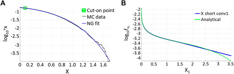
FIGURE 1. (A) NG fit of the MC-simulated Duffing response for ${\mathit{f}}_{\mathit{X}}$. (B) Deconvoluted distribution, linearly extrapolated (blue) ${\mathit{f}}_{{\mathit{X}}_{\mathit{1}}}$versus the analytic solution (green).

Finally, there is a note regarding the issue with the interpolation of the «shorter» data record distribution tail $f_X$. The latter interpolation was necessary because the empirical $f_X$ distribution is naturally highly irregular at the terminal tail section, thus making the empirical $f_X$ distribution unsuitable input for Eq. 4. Therefore, this study adopted a simple convex (logarithmic scale) NG (Naess–Gaidai) interpolation form

with a proper optimization technique for minimizing the following function F with respect to $a,b,c,\mathrm{a}\mathrm{n}\mathrm{d}d$. F is the mean square error function and $a,b,c,\mathrm{a}\mathrm{n}\mathrm{d}d$ are constants. More details can be found in the reports by Naess and Moan (2013) and Zhang et al. (2019).

where $x_0$ is the tail marker indicating the beginning of the extrapolation tail area (green squares in Figure 3). The weight function $w$ may be defined in various ways; e.g., as $w\left(x\right)={\left\{\ln C^{+}\left(x\right)-\ln C^{-}\left(x\right)\right\}}^{-2}$. $\left(C^{-}\left(x\right),C^{+}\left(x\right)\right)$ is the confidence interval (CI). Simulated or measured data can be used to empirically estimate the CI. The main difference in this study, as compared to Naess and Moan (2013) and Zhang et al. (2019), is that there is no extrapolation using Eq. 6, only interpolation. Note that any other log-convex interpolation form, different from Eq. 6, would also work. The Levenberg–Marquardt non-linear least-squares algorithm (Kanzow et al., 2004; Lourakis, 2004; Numerical Algorithms Group, 2010) was used to find the optimal fit parameters $a,b,c,d$.

Synthetic example: Non-linear Duffing oscillator

In this section, a non-linear Duffing oscillator that is subjected to Gaussian white noise has been used as an example to validate and benchmark the proposed method. The mean up-crossing rate ${\nu }_X$ of the Duffing oscillator response to a stochastic loading was chosen as the target function $f_X$ to study its distribution tail properties, similar to the previous section. Note that in this case $f_X$ was not a probability distribution but is rather a scaled mean up-crossing rate function closely related to extreme response statistics.

As the first example system, we used the ubiquitous single-degree-of-freedom Duffing oscillator excited by stationary Gaussian white noise W(t)

with $\delta$($\tau$) indicating the $\delta$-function. That is, the Duffing oscillator equation takes the specific form

where for the present example $\epsilon$ = 1, $\beta$ = 0.2 were chosen. This choice of $\epsilon$ makes the Duffing oscillator strongly non-linear. This model is attractive for illustration purposes because the mean up crossing rate is in closed form (later in this study called «analytic solution»), thus offering an easy way of verifying the extrapolation approach.

The left side of Figure 1 presents the NG fit of the MC simulated Duffing response. The right side shows the deconvoluted distribution, linearly extrapolated versus analytic solution. The deconvoluted function $f_{X_1}$ is more linear in the tail than the original target function $f_X$.

Figure 2 presents the results of the comparisons between the deconvolution method, analytic, and NG for the target function $f_X$. The proposed deconvolution method performed significantly better than the NG extrapolation.

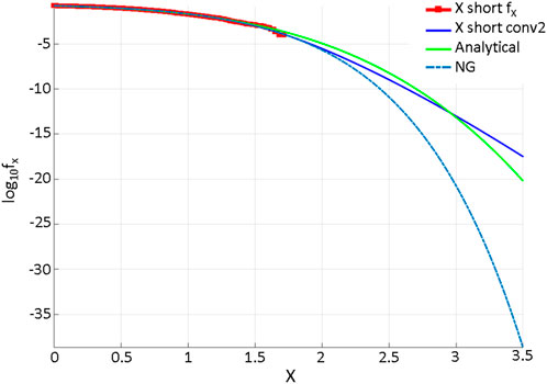
FIGURE 2. Comparison of deconvolution methods (solid blue), analytic (green), and NG (dashed blue). The MC-simulated response is indicated in red (*).

Deck panel stresses on container ships

This section illustrates the efficiency of the proposed method applied to actual onboard data measured on container vessels. The accurate prediction of extreme stresses in ships is essential. Serious accidents have involved ships breaking apart during voyages. The MSC Napoli (ClassNK, 2014) and MOL Comfort (MAIB, 2008) are two such Post-Panamax container ships that broke apart during their voyages in January 2007 and June 2013, respectively. Both ships broke due to overloading at the hull girder in the midship area. The investigation reports are presented in (ClassNK, 2014)- (MAIB, 2008).

Figure 3 shows a vessel similar to that considered in this study. This TEU2800 container ship is a 245 m long Panamax vessel that was instrumented in August 2007. The routes taken by the ship between 2007 and 2010 are shown in Figure 4. Figure 4 also shows the alterations to the route to avoid severe storms; i.e., the ship sails around some areas to avoid storms in those locations.

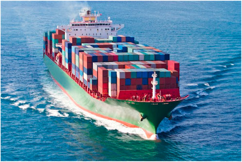
FIGURE 3. Example of a loaded TEU container vessel (Gaidai et al., 2022).

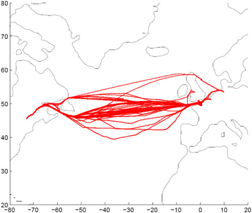
FIGURE 4. North Atlantic routes, 2007—2010 (Gaidai et al., 2022).

Figure 5 shows the location of the strain gauges installed in the mid-ship area, where the ships normally experience the largest stresses and, as mentioned above, where the MSC Napoli and MOL Comfort broke apart. The same figure also illustrates the locations where cracks were observed. The strain gauges are installed according to the DNV container vessel rules and regulations (DNV, 2005; DNV, 2009; DNV, 2015; DNV, 2018a; DNV, 2018b). The strain gauges are aligned along in the vessel’s fore-aft direction thus, the measures strains and stresses measured are aligned in the longitudinal direction of the ship.

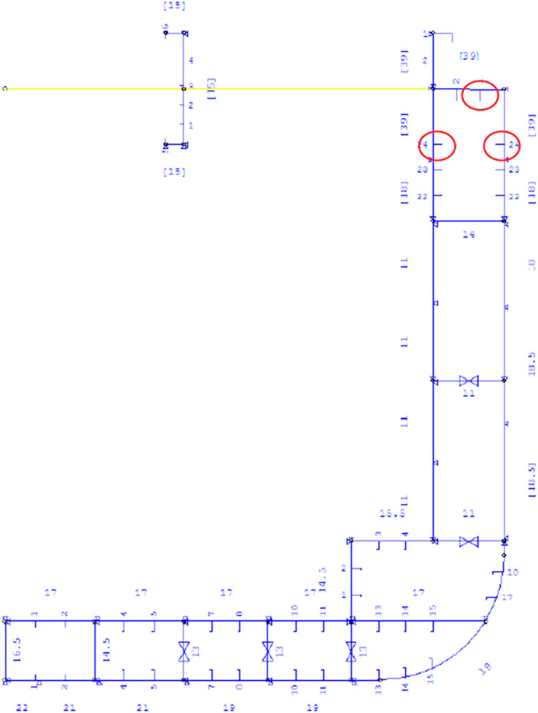
FIGURE 5. Layout of the mid-ship cross-section showing the measurement position in the upper deck and crack positions at stringer level 1 (Gaidai et al., 2022).

Figure 6 presents over 70 available time series of measured onboard DMP (deck mid port) stress during trans-Atlantic voyages. The «shorter» data record was generated by taking the tenth data point from the «longer» deck panel stress data record. Therefore, the «shorter» data record had an equivalent time length of only 1 year.

FIGURE 6. Time series of combined measured onboard stress.

The left side of Figure 7 presents the «shorter» data record $f_{X_1}$ tail, obtained by deconvolution as in Eq. 2, and subsequently linearly extrapolated in the terminal tail section to cover the $X_1$ range matching the «longer» data record. The right side of Figure 7 presents the final unscaled results of the proposed technique; namely, the «shorter » decimal log scale $f_X$ tail, extrapolated by deconvolution, along with the «longer» data distribution tail and Naess–Gaidai (NG) extrapolation.

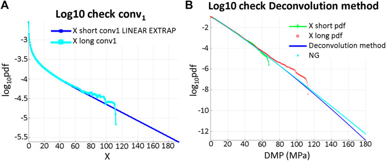
FIGURE 7. DMP stress. (A) Scaled${\mathit{f}}_{{\mathit{X}}_{\mathit{1}}}$ tail on a decimal log scale for the «shorter» data (cyan), linearly extrapolated (dark blue). (B) Unscaled raw «shorter» data (green) ${\mathit{f}}_{\mathit{X}}$ tail on a decimal log scale, extrapolated by deconvolution method (dark blue), along with «longer» raw data (red) and NG extrapolation (cyan).

The right side of Figure 7 shows that the proposed method performs well, being based on the «shorter» data set and presenting a distribution quite close to the one based on the «longer» data set.

Conclusion

The results of the present study showed the practical advantages in the application of the proposed deconvolution method. The main advantage of this method is that, unlike most engineering fit methods, it is based on the intrinsic properties of the data set itself and does not assume any extrapolation functional class. To highlight the accuracy and effectiveness of the method, this study analyzed both synthetic and real onboard measured ship panel stress data sets. The prediction accuracy of the proposed method was validated versus the Naess–Gaidai method.

For the synthetic Duffing case, the predictions obtained by the proposed method showed better agreement with the analytical solution compared to the prediction using the Naess–Gaidai method.

The proposed method performed well in the measurement of onboard measured ship panel stress. The NG method predictions agreed with those of the proposed method in this example.

The results of this study demonstrated that the novel deconvolution method for particular cases increased the prediction accuracy of extreme onboard measured ship panel stress. The proposed method is unbiased regarding any pre-chosen fitting functional class, which can be useful in engineering applications where more accurate unbiased characteristic design values are essential. Moreover, the proposed technique is not limited to only the prediction of extreme onboard measured ship panel stress, as it has general potential in naval architecture and offshore engineering applications. For example, this extrapolation method could also be used to predict fatigue life (Gaidai et al., 2020).

Data availability statement

The raw data supporting the conclusion of this article will be made available by the authors, without undue reservation.

Author contributions

All listed authors have made substantial, direct, and intellectual contributions to the work and have approved its publication.

Funding

This study was partially supported by the National Natural Science Foundation of China (grant number: 52071203).

Acknowledgments

The authors express their gratitude for the support from the Fishery Engineering and Equipment Innovation Team of Shanghai High-level Local University. The authors also thank the owner, manager, superintendents, masters, and crew for their assistance in obtaining the measurement data. Further thanks to DNV for the support and sharing of measurement data for this research.

Conflict of interest

The authors declare that the research was conducted in the absence of any commercial or financial relationships that could be construed as a potential conflict of interest.

Publisher’s note

All claims expressed in this article are solely those of the authors and do not necessarily represent those of their affiliated organizations, or those of the publisher, the editors, and the reviewers. Any product that may be evaluated in this article, or claim that may be made by its manufacturer, is not guaranteed or endorsed by the publisher.

References

Berge, E., Byrkjedal, O., Ydersbond, Y., Kindler, D., and Kjeller Vindteknikk, A. S. (2009). Modelling of offshore wind resources. Comparison of a meso-scale model and measurements from FINO 1 and North Sea oil rigs. EWEC 2009, 1–8.
ClassNK, 2014, Investigation report on structural safety of large container ships", the investigative panel on large container ship safety, Available at: http://www.classnk.or.jp/hp/pdf/news/Investigation_Report_on_Structural_Safety_of_Large_Container_Ships_EN_ClassNK.pdf.
DNV (2015). Fatigue assessment of ship structures. DNV Classification Note CG-0129. Hølvik, Norway: DNA.
DNV (2018a). Fatigue assessment of ship structures. DNV GL class guideline DNVGL-CG-0129. Hølvik, Norway: DNA.
DNV (2009). Hull structural design, ships with length 100 meters and above, DNV Rules for Classification of Ships. Hølvik, Norway: DNA.
Gaidai, O., and Naess, A. (2008). Extreme response statistics for drag dominated offshore structures. Probabilistic Eng. Mech. 23 (2-3), 180–187. doi:10.1016/j.probengmech.2007.12.012
Gaidai, O., Naess, A., Karpa, O., Xu, X., Cheng, Y., and Ye, R. (2019). Improving extreme wind speed prediction for North Sea offshore oil and gas fields. Appl. Ocean Res. 88, 63–70. doi:10.1016/j.apor.2019.04.024
Gaidai, O., Naess, A., Xu, X., and Cheng, Y. (2019). Improving extreme wind speed prediction based on a short data sample, using a highly correlated long data sample. J. Wind Eng. Industrial Aerodynamics 188, 102–109. doi:10.1016/j.jweia.2019.02.021
Gaidai, O., Storhaug, G., Naess, A., Ye, R., Cheng, Y., and Xu, X. (2020). Efficient fatigue assessment of ship structural details. Ships Offshore Struct. 15 (5), 503–510. doi:10.1080/17445302.2019.1661623
Gaidai, O., Storhaug, G., Wang, F., Yan, P., Naess, A., Wu, Y., et al. (2022). “On-board trend analysis for cargo vessel hull monitoring systems,” in The 32nd International Ocean and Polar Engineering Conference, Shanghai, China, June 6, 2022–June 10, 2022.
Gaidai, O., Xu, X., Naess, A., Cheng, Y., Ye, R., and Wang, J. (2021). Bivariate statistics of wind farm support vessel motions while docking. Ships Offshore Struct. 16 (2), 135–143. doi:10.1080/17445302.2019.1710936
Hui, G., Gaidai, O., Naess, A., Storhaug, G., and Xu, X. (2019). Improving container ship panel stress prediction, based on another highly correlated panel stress measurement. Mar. Struct. 64, 138–145. doi:10.1016/j.marstruc.2018.11.007
Kanzow, C., Yamashita, N., and Fukushima, M. (2004). Levenberg–Marquardt methods with strong local convergence properties for solving nonlinear equations with convex constraints. J. Comput. Appl. Math. 172 (2), 375–397. doi:10.1016/j.cam.2004.02.013
Karpa, O. (2012). ACER user guide. Available at: http://folk.ntnu.no/karpa/ACER/ACER_User_guide.pdf.
Lourakis, M. I. (2004). levmar: Levenberg-Marquardt nonlinear least squares algorithms in C/C++. Available at: http://www.ics.forth.gr/∼lourakis/levmar/.
MAIB (2008). “Report on the investigation of the structural failure of MSC Napoli English channel on 18th january 2007,”. Report No. 9/2008, April 2008 in Marine accident investigation branch (MAIB) (Carlton Place, Southampton, UK, SO15 2DZ: Carlton House). Available at: https://www.gov.uk/maib-reports.
Naess, A. (1998). Estimation of long return period design values for wind speeds. J. Eng. Mech. 124 (3), 252–259. doi:10.1061/(asce)0733-9399(1998)124:3(252)
Naess, A., Gaidai, O., and Batsevych, O. (2010). Prediction of extreme response statistics of narrow-band random vibrations. J. Eng. Mech. 136 (3), 290–298. doi:10.1061/(asce)0733-9399(2010)136:3(290)
Naess, A., Gaidai, O., and Haver, S. (2007). “Estimating extreme response of drag dominated offshore structures from simulated time series of structural response,” in International Conference on Offshore Mechanics and Arctic Engineering, San Diego, CA, 99–106.42681
Naess, A., and Gaidai, O. (2008). Monte Carlo methods for estimating the extreme response of dynamical systems. J. Eng. Mech. 134 (8), 628–636. doi:10.1061/(asce)0733-9399(2008)134:8(628)
Naess, A., and Karpa, O. (2015). Statistics of extreme wind speeds and wave heights by the bivariate ACER method. J. Offshore Mech. Arct. Eng. 137 (2), 4029370. doi:10.1115/1.4029370
Naess, A., and Moan, T. (2013). Stochastic dynamics of marine structures. Cambridge: Cambridge University Press.
Naess, A., Stansberg, C. T., Gaidai, O., and Baarholm, R. J. (2009). Statistics of extreme events in airgap measurements. J. offshore Mech. Arct. Eng. 131 (4). doi:10.1115/1.3160652
Naess, A. (1998). Statistical extrapolation of extreme value data based on the peaks over threshold method. J. Offshore Mech. Arct. Eng. 120, 91.
Næss, A., and Gaidai, O. (2009). Estimation of extreme values from sampled time series. Struct. Saf. 31 (4), 325–334. doi:10.1016/j.strusafe.2008.06.021
Perrin, O., Rootzén, H., and Taesler, R. (2006). A discussion of statistical methods used to estimate extreme wind speeds. Theor. Appl. Climatol. 85 (3), 203–215. doi:10.1007/s00704-005-0187-3
Pickands, J. (1975). Statistical inference using extreme order statistics. Ann. Statistics 1975, 119–131.
Valberg, M. (2010). Aspects of applying the ACER method to ocean wave data Master's thesis. (Trondheim, Norway: Institutt for matematiske fag).
Xu, X., Gaidai, O., Naess, A., and Sahoo, P. (2019). Improving the prediction of extreme FPSO hawser tension, using another highly correlated hawser tension with a longer time record. Appl. Ocean Res. 88, 89–98. doi:10.1016/j.apor.2019.04.015
Keywords: deconvolution, reliability, container vessel, ship panel stress, trans-Atlantic voyage
Citation: Gaidai O, Yan P and Xing Y (2022) Prediction of extreme cargo ship panel stresses by using deconvolution. Front. Mech. Eng 8:992177. doi: 10.3389/fmech.2022.992177
Received: 12 July 2022; Accepted: 29 August 2022;
Published: 30 September 2022.
Edited by:
Fuyin Ma, Xi’an Jiaotong University, ChinaReviewed by:
Guobiao Hu, Nanyang Technological University, SingaporeXiaosen Xu, Jiangsu University of Science and Technology, China
Jinqiang Li, Harbin Engineering University, China
Copyright © 2022 Gaidai, Yan and Xing. This is an open-access article distributed under the terms of the Creative Commons Attribution License (CC BY). The use, distribution or reproduction in other forums is permitted, provided the original author(s) and the copyright owner(s) are credited and that the original publication in this journal is cited, in accordance with accepted academic practice. No use, distribution or reproduction is permitted which does not comply with these terms.
*Correspondence: Yihan Xing, yihan.xing@uis.no
†These authors contributed equally to this work