General Multi-Fidelity Framework for Training Artificial Neural Networks With Computational Models

Introduction

Over the last years, we have witnessed several groundbreaking advances in artificial intelligence (AI) that were based on a simple idea: a virtual training environment was created by setting up some general rules. Subsequently, an AI, typically represented by an artificial neural network (ANN), was placed in this training environment and allowed to practice until it reached a superhuman level of mastery. The rules of the training environment were, for example, the rules of the board game Go in the AlphaGo project (Silver et al., 2016). Even when the machine learning component was not provided any prior knowledge about the game other than the ruleset itself it achieved superhuman mastery simply by training in a virtual training space (Silver et al., 2017). Other research projects rely on virtual environments as used in computer games in order to train AIs to perform intelligent actions or solve certain problems (Vinyals et al., 2017). This research typically uses training environments defined by rules whose complexity is far below that of real physics. Consequently, the generation of training data is feasible at such a low computational cost that one can apply straightforwardly a Big Data paradigm, in which the training of the ANN is the bottleneck, not the availability of data. With physically more realistic virtual training environments one could train AIs to solve problems, for example, from mechanical engineering or materials science that require so far intense human interactions. Creating physically realistic models of systems and processes in mechanical engineering and materials science is the principal objective of computational mechanics. It is thus natural to combine computational mechanics and machine learning to create what one may refer to as “computational mechanics intelligence,” that is, a kind of artificial/computational intelligence that is endowed with an accurate understanding of a certain mechanical problem and which is trained in a virtual environment created by methods from computational mechanics. This paradigm can actually be understood as a natural extension of the fast growth body of research that seeks to apply machine learning to various areas of mechanical engineering or materials science such as fatigue (Mosallam et al., 2016; Wang et al., 2017), homogenization (Yang et al., 2018), or process design (Hu et al., 2018). The idea to couple computational mechanics and artificial intelligence in an intimate way bears great promise to open up new ways to endow AI with an understanding of real physics. However, it faces the great challenge that creating training data for an AI by means of realistic models of complex physical systems and processes can be computationally prohibitively expensive. This is a main reason why the attempts to couple computational mechanics and artificial intelligence–although started first already long ago (cf. Waszczyszyn and Ziemianski, 2001)–have so far remained very limited both in scope and number. The key to the future success of computational mechanics intelligence is thus developing smart strategies how computational models can be used to train AIs at an acceptable overall computational cost. If realistic computational models are used for training AIs, the computational cost of the models typically by far surpasses the computational cost of the AI training itself. It is thus of paramount importance to find ways to reduce in particular the computational cost associated with the generation of training data by means of computational models. In the area of computational quantum mechanics, recently a variable-fidelity method for the calculation of bandgaps was proposed (Pilania et al., 2017). Apparently, it is promising to combine also for classical computational mechanics on the continuum scale simulations with multiple different fidelity levels in order to reduce computational cost for generating training data. In this paper, we will introduce a systematic and general framework how to use computational methods in a smart way in order to create training data for AIs. This framework relies on a multi-fidelity strategy which couples the learning progress of the AI with the resolution of the computational models used to generate training data. It trades unnecessary precision of the error gradient used especially in the early stages of AI training for computational efficiency. The main objective of our multi-fidelity strategy is to significantly speed up the training of ANNs in domains in which training data have to be generated by means of computational models and where this process constitutes a significant portion of the overall computational cost associated with endowing an AI with physical intelligence. The outline of the paper is as follows. In section “Problem setting,” we briefly describe the type of problem on which this article focuses. In section “Methods,” we delineate the architecture and general learning algorithms of the ANNs used in this paper. Moreover, we introduce our novel multi-fidelity framework for coupling computational models and AI training. In section “Numerical Examples,” we demonstrate the benefits of this multi-fidelity framework using examples from both structural mechanics and materials mechanics. Finally the section “Conclusions” summarizes and discusses the broader implications of the multi-fidelity framework introduced herein.

Problem Setting

Herein we consider the following general problem: an AI is to be trained to perform some kind of action or make some kind of prediction within or with respect to a physical system. Experiments with and measurement within the physical system in order to generate training data for the AI are assumed to be expensive, time-consuming, or dangerous so that it is preferable to generate training data rather by means of “simulated experiments” or “simulated measurements” performed by means of a realistic computational model of the physical system of interest. The computational cost of these simulated experiments is assumed to surpass by far the computational cost of AI training on the basis of given training data itself. It is therefore the bottleneck in coupling artificial intelligence and computational models. The general problem delineated above mainly appears in two settings. In the first one, the AI is used to make predictions about the behavior of a physical system under variable input. The motivation may be that using a comprehensive classical computational model for making these predictions for each different input case of interest may be much more expensive than using an AI as a cheap surrogate model. In this setting, the computational model is used to compute for a large number of input values realistic approximations of the associated output of the system. These input and computationally approximated output values form together training samples which can be used for training an AI to approximate the behavior of the computational model. Typically, this is achieved by means of a backpropagation training algorithm where the internal parameters of the AI are adjusted until for a given input the AI produces an output sufficiently similar to the one of the computational model. This adjustment is based on the current error of the AI, that is, the current deviation of the AI output from the output of the computational model for a certain input (cf. Figure 1, left).

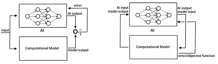
Figure 1. Left: training an AI as a cheap surrogate model of a classical computational model in order to make predictions about input-output relations in a physical system or process. The difference between AI output and model output is an error that can be used for AI training (e.g., using backpropagation algorithms). Right: AI is used to take action in or control a physical environment or parts of it. The error controlling AI training has to be computed in some way from the AI-governed evolution of the computational model (e.g., using some objective functions assessing the current or final state of the computational model).

In the second problem setting, the AI is to be trained to take action in a specific physical environment. To this end, the AI is connected, typically in a closed-loop setting, to a computer simulation of this physical environment in which actions and consequences can be evaluated much faster and cheaper than in real-world experiments (cf. Figure 1, right). This setting becomes relevant, for example, if an AI should be used to control complex processes and systems such an autonomously driving car or an autonomously flying drone or robots in a manufacturing plant. The difference between this setting and the first one is mainly that the input to the AI cannot be arbitrarily chosen already before starting the training but typically results–at least in parts–only in the course of the training process as a consequence of closed-loop interactions between AI and computational model. Moreover, AI training can typically not be simply based on a difference between AI output and model output but will rather more often rely on some objective function evaluated on the current state of the system.

Despite these differences, both the above problem settings have in common that AI training requires the evaluation of computationally expensive models. In the next section we will delineate a multi-fidelity strategy that can heavily alleviate the associated computational cost, which otherwise is often prohibitively high for realistic computational models of complex systems. While the general concept of this strategy applicable to both the above delineated problem settings, we will focus in this article on the first problem setting illustrated in Figure 1, left.

Methods

Architecture of Artificial Intelligence

ANNs are chosen as the most general-purpose, widely spread type of learning algorithm. This choice is taken as to minimally constrain the generalizability of the multi-fidelity approach introduced in this research. The specific ANNs used herein are feed forward neural networks (FFNs) based on several densely connected hidden layers. Their learning process thus falls into the realm of so-called deep learning. This choice is not mandatory, and it is important to note that other choices of the machine learning algorithm would be equally viable to exemplify the comparative advantages of the multi-fidelity framework developed herein. While the results of this research are not wholly agnostic with respect to the choice of learning algorithm and specific parameters (learning rate, activation functions, etc.), the above choice has been made so as to maximize the generalizability of the results obtained herein and not make them merely an artifact of a peculiarity of the highly specific learning method.

Learning Algorithm

There are various different ways how ANNs can be trained to imitate a function, the most common of which is supervised learning. Even though there is a host of different approaches to supervised learning with differences ranging from small details to entirely different architectures, all these approaches share a couple of common elements. In general, supervised learning algorithms compare the current output of an ANN for a given input with the correct solution, and base the correction of the internal parameters of the neural network (i.e., the “learning”) on an error which is the difference between current and correct output. Although there are also derivative-free methods, correcting the internal parameters of the network in most approaches requires the computation of a gradient the said error with respect to the parameters governing directly the output of the ANN. In a so-called “backpropagation algorithm” this gradient is propagated through the ANN and used to update thresholds/weights for the individual neurons in the ANN.

To train the ANN, a large amount of training data is required. Each training sample consists of one tuple of an input (to the computational model or the ANN) and the corresponding output which the ANN should learn to ideally yield in response to the respective input values. In our setting the output which the ANN should learn to reproduce is generated by means of a computational model. Our objective is training the ANN to reproduce the input-output behavior of the computational model. To this end, the ANN is fed one training sample after the other. In supervised learning (i.e., when the desired output for specific input to the ANN can at least in principle be computed from the beginning on), training samples are typically not used individually for backpropagation training but rather the error and error gradients used for backpropagation training are computed across so-called batches of N samples and then used. This reduces computational cost and perturbations of the learning process due to specific numerical features of individual samples. The error over a batch of N training samples is computed in our framework as a root mean square error (RMSE) (Russell and Norvig, 2016).

with ŷ_i the results predicted by the ANN for the input of sample i within the training batch, and y_i the corresponding output provided by the computational model. The error gradient, which is needed for backpropagation training, can be computed by a simple finite-difference-like approximation of the derivatives of (1).

Multi-Fidelity Training

General Idea

Typical algorithms for AI training such as gradient-based backpropagation algorithms for ANNs are realized by way of a process where the internal parameters of the ANN are adjusted in a stepwise, iterative manner to improve its performance. When ANN training starts, mainly a coarse adjustment of the internal parameters of the ANN toward reasonable values takes place because a tailor-made problem-specific initialization of these parameters is typically not possible. This way, the AI is endowed with a first coarse understanding of the basic properties of the problem to which it is applied. Only later on the ANN is fine-tuned. In this process, the initial adjustments of the internal parameters of the ANN need not be accurate because in subsequent training steps their precise values will still change in a way that cannot directly be foreseen in the beginning. Small perturbations of the initial steps can thus be expected to remain without major impact on the overall result of the training process. Thus, it is sufficient if during the initial training stage the internal parameters of the ANN are altered in a way which points roughly in the right direction. To this end, it is sufficient to use in the initial stage of ANN training samples generated by means of coarse low-fidelity computational models, which may exhibit considerable numerical approximation errors but which are computationally cheap. Only later on, as ANN training progresses one has to gradually move toward samples generated by means of more accurate and computationally more expensive higher-fidelity models. Following this strategy one can use cheap low-fidelity samples for a large part of the ANN training and needs computationally expensive high-fidelity samples only in the very end of the training process and thus only in a very limited number. Exploiting such a multi-fidelity strategy, which is illustrated in Figure 2, can substantially reduce the overall computational cost (compared to a non-optimized brute-force training of the ANN). It is worth emphasizing that the main objective of this multi-fidelity strategy is indeed reduction of the computational cost for training ANNs to a given level of accuracy rather than training ANNs more accurately. Precisely, our multi-fidelity framework is based on the following course of action. We first define a number of different fidelity levels along with associated computational models. We start generating training data for the ANN using the computational model with lowest fidelity. We continue using the low-fidelity model as long as the overall performance of the ANN increases and we can expect that using the a computational model at the current level of fidelity can help to train the ANN in an efficient way. As soon as this is no longer the case, we move on toward higher fidelity training data. In practice, this is typically possible by simply using computational models based on a finer discretization. More details on this will be given below.

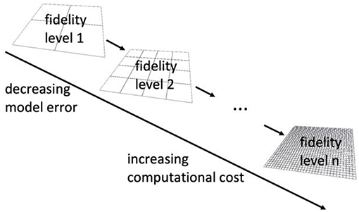
Figure 2. In our multi-fidelity framework we use computational models with different fidelity (accuracy) of one and the same physical system or process. Different fidelity levels can in the context of most computational schemes easily be realized by variations of the discretization length. Finer discretization typically yields more accurate but computationally also more expensive models. Thus, it is favorable to use as many samples as possible at lower fidelity levels in order to pre-train an ANN before a much smaller number of accurate high-fidelity samples is used for fine-tuning the internal parameters of the ANN.

For simplicity we focus in the discussion herein and in particular in the examples section on ANNs as a widely used basis for AI and on computational models based on the finite element method, which is widely used both in solid and fluid mechanics as well as many other areas of continuum physics. We stress, however, that we expect the multi-fidelity strategy introduced herein to be generalizable also to cases where the computational models used are not based on finite-element discretizations or where more complex or specialized machine learning architectures are used than ANNs. In fact, we expect the multi-fidelity strategy introduced in this paper to be applicable as long as the following three conditions are satisfied. First, there must be a necessity to generate training data for the AI by means of computational models. Second, the computational expense of generating training data using these models should vastly exceed the computational expense of training the AI itself. Third, it must be possible to create for the physical system or process of interest computational models with varying levels of accuracy, lower levels of accuracy thereby being associated also with a lower computational cost.

Criteria for Switching to Higher Fidelity Levels During Training

In standard-problems of supervised learning, all training data are available from the beginning on. In this case, the training data can be divided into batches and the following course of action is common: all batches are fed into the ANN, whereby, however, from each batch only 90% of the samples are used for training and 10% are retained for validation purposes. Once all batches have been fed into the ANN a so-called epoch is completed. At this point the RMSE with respect to the samples retained for validation is computed. Subsequently, the next epoch starts where again all batches are fed into the ANN. This sequence is interrupted, however, as soon as the RMSE computed for the validation samples after an epoch has increased compared to the previous epoch. The motivation for this strategy is the avoidance of overfitting (Domingos, 2012; Russell and Norvig, 2016), which is a tendency of learning algorithms not to learn the intended, generalizable target function but rather features of the specific training data unless the training process for a given set of data is stopped in time. Once the RMSE for the validation samples–which were not used for training and are unknown to the ANN–starts to increase, even though the RMSE for the training data themselves may still continue to decrease, overfitting can be assumed to start.

In our setting, we have to pursue a slightly modified course of action. The reason is that the complete set of training data is not available from the beginning on but rather has to be generated during learning because in the beginning it is not even known how many training samples have to be generated from computational simulations in order to achieve a reasonable performance of the ANN. To overcome this problem, we start our training with data generated by means of a computational model at the lowest fidelity level. We generate one or several batches of training data, depending on criteria discussed in more detail below. In each batch, we retain 10% of the samples for validation and use the remaining 90% for training. We train the ANN looping in a batch-wise manner through all the training samples. Looping one time through all available training samples is called an epoch. We do so again and again and complete this way more and more epochs until either a certain predefined maximal number E of epochs has been completed or until the RMSE based on the validation samples increases (which is a sign of overfitting). Once this point is reached, a so-called super-epoch is considered to be completed. After each super-epoch, we evaluate the recent training progress of the ANN. We do so on the basis of two quantities. The first quantity is the current RMSE of the ANN

on the basis of $\bar{N}$ output values $\left\{y_i^{\mathrm{\text{max}}}\right\}$ which are generated in the very beginning of the whole training process using a computational model at the highest fidelity level and which are never used for training.

To obtain the second quantity required to evaluate the recent training progress of the ANN at the current fidelity level i, we compute an estimate of the approximation error of the computational model at this fidelity level. To this end, we assume that accuracy differences between the highest fidelity level at which the computational model is available and the lowest one with i = 1 are very large so that we can approximate the approximation error of the computational model at the lowest fidelity level with i = 1 as

where $\left\{y_i^1\right\}$ and $\left\{y_i^{\mathrm{\text{exact}}}\right\}$ are the output values which a computational model with the lowest fidelity level and a fictitious exact model of the physical system of interest yield when provided the same input values that make the computational model at the highest fidelity level yield the above introduced $\left\{y_i^{\mathrm{\text{max}}}\right\}$. $O(e_{\mathrm{\text{CM}}}^{max})$ is a term on the order of magnitude of the RMSE of the computational model at the highest fidelity level compared to the fictitious exact model. We assume now that the modeling error of the computational model at fidelity level i is governed by the discretization lengths h_i used in the computational model, and that it converges monotonically to zero with the p-th power of h_i. Then the error of the computational model at the i-th fidelity level can be estimated as

The training progress after a super-epoch is always considered unsatisfactory if the following criterion applies:

(T1) The RMSE $e_{\mathrm{\text{ANN}}}^{\mathrm{\text{max}}}$ according to (2) after the current super-epoch is worse than the RMSE s super-epochs ago.

Criterion (T1) indicates that the ANN is no longer learning general features of the problem but rather batch-specific information. We average the RMSE over the last s super-epochs when monitoring the training progress in order to reduce the impact of random fluctuations during a single super-epoch. Depending on the exact training strategy (cf. section “Different Training Strategies” for more details) one may consider the training progress after a super-epoch also unsatisfactory if the following additional criterion applies:

(T2) The RMSE $e_{\mathrm{\text{ANN}}}^{\mathrm{\text{max}}}$ according to (2) after a super-epoch is smaller or equal than q times the approximation error $e_{\mathrm{\text{CM}}}^i$ of the computational model at the current fidelity level estimated on the basis of (4).

Criterion (T2) indicates that the ANN has been trained to a level of accuracy comparable to the one of the computational model at the current fidelity level. Naturally, training beyond this level is impossible and q can be understood as a safety factor which ensure that training always stops earlier, taking into account that (4) is just a rough estimate.

If the training progress after a super-epoch is found to be satisfactory on the basis of criteria such as (T1) and possibly also (T2), we continue training at the same fidelity level. Otherwise, we switch to the next higher fidelity level. If there is no higher fidelity level, we terminate training.

Different Training Strategies

In this paper, we compare altogether three different training strategies. The first one is a simple single-fidelity approach where the whole training of the AI is based on samples generated at the same (maximal) level of fidelity and thus also computational cost. As viable alternatives to this simple brute-force approach, which is most widely practiced so far, we propose and compare in the following also two different multi-fidelity strategies.

Single-Fidelity Training

Training ANNs with data generated from computational models is so far mostly performed in a single-fidelity paradigm where all training data are generated with the same computational model and thus with the same fidelity level. Therefore, we test this approach also herein as a benchmark to measure the performance gains that can be achieved by the multi-fidelity framework introduced herein. To ensure comparability between single-and multi-fidelity training, single-fidelity training is terminated as soon as either criterion (T1) from section “Criteria for switching to higher fidelity levels during training” is satisfied or the RMSE of the ANN has decreased to a threshold RMSE_min which is chosen to be equal to $q{e}_{\mathrm{\text{CM}}}^i$ from criterion (T2) in the multi-fidelity training algorithm with which the single-fidelity training algorithm is compared. The algorithm for single-fidelity training is provided as pseudocode in Table 1.

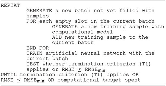
Table 1. Pseudocode for single-fidelity training.

Unidirectional Multi-Fidelity Training

In the simplest “brute-force” multi-fidelity approach, we unidirectionally loop through different fidelity levels. We start at the lowest one and move on to the next higher fidelity level as soon as one of the two termination criteria (T1) and (T2) from section “Criteria for Switching to Higher Fidelity Levels During Training” are satisfied. If this happens on the highest fidelity level, we terminate training completely. Before starting the training process, we have to define the number n of fidelity levels as well as the computational models assigned to them. When using finite element discretizations as we do herein, one can create computational models at n different fidelity levels simply by starting at the lowest fidelity level and refining then from one fidelity level to the next one the discretization mesh by a certain factor (e.g., a factor of two or four). The algorithm for unidirectional multi-fidelity training is provided as pseudocode in Table 2.

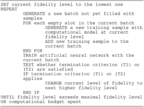
Table 2. Pseudocode for unidirectional multi-fidelity training.

Bidirectional Multi-Fidelity Training

In the brute-force multi-fidelity approach switching to a higher fidelity level is based on the criteria (T1) and (T2) from section “Criteria for switching to higher fidelity levels during training” and it is irreversible. Evaluation of criterion (T2) requires the approximation (4). In certain cases, this approximation may exhibit an unusually high error, for example, because the errors of the computational models at the different fidelity levels are not related by a simple power law. This happens in practice in particular if the lowest fidelity levels are based on extremely coarse discretizations because simple power laws governing convergence mostly apply only in the limit of infinitesimal (or practically at least relatively fine) discretization lengths. If (4) exhibits a high error, application of (T2) may lead to a strongly reduced computational efficiency. To overcome this problem, one can skip in such cases termination criterion (T2) as a whole and rather adopt the following bidirectional approach for switching between different fidelity levels: at a given fidelity level one first generates one batch at the next higher and one batch at the next lower fidelity level (if these exist) as well as several batches at the given fidelity level. The number of batches at the given fidelity level is adjusted such that the computation time spent on the generation of these batches surpasses the one spent for the generation of the single batch at the next higher fidelity level by a factor of m > 1. In the following we always assume m = 4, noting that the exact choice of m has only minor impact. Higher choices for m would reflect a lower rate at which the learning efficiency per computational resource is compared between fidelity levels. However, as additional batches at the comparatively lower fidelity level only gradually diminish their contribution to the learning process, our results were insensitive to delayed comparisons (and thus delayed transitions to a different fidelity level) as reflected by higher choices of m.

This procedure ensures that at each fidelity level one spends by far most of the computation time on generating training samples at this very fidelity level but that one also has available one “trial” batch at the next higher and next lower fidelity level, respectively. Now one uses the generated batches at these three fidelity levels for training the ANN subsequently in three super-epochs. For each fidelity level, we valuate the ratio between the reduction of the RMSE during the associated super-epoch and the computation time spent on generating the underlying training samples. The fidelity level for which this ratio is maximal is chosen as the new “current” fidelity level. Note that this rule admits not only increasing the fidelity level but also decreasing it in case that this is found to be computationally beneficial. For the sake of clarity, the bidirectional multi-fidelity strategy is described in detail as pseudocode in Table 3.

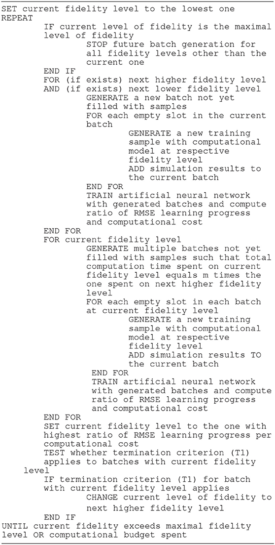
Table 3. Pseudocode for bidirectional multi-fidelity training.

The bidirectional multi-fidelity strategy completely bypasses termination criterion (T2) and replaces it by a smart, bidirectional switching strategy between different fidelity levels which ensures that the vast majority of computational time is always spent on samples at the fidelity level that currently enables the computationally most efficient learning. It is worth mentioning that bidirectional multi-fidelity training can be particularly useful if the computational models used at the different global fidelity levels exhibit an approximation error that strongly depends on the input parameter regime so that for certain choices of input parameters the fidelity (in terms of an absolute model error) is much higher than for others. If one generates in such cases samples with input values which are not randomly distributed but which for example first probe one parameter regime with a relatively high approximation error of the computational model and subsequently another input parameter regime with a relatively low approximation error of the computational model, it will typically be efficient to reduce the global fidelity level if one moves from the first to the second input parameter regime because this would actually ensure that the approximation error of the training samples remains rather constant when switching from one to the other regime, which is beneficial because this approximation error should be linked to the smoothly changing approximation performance of the ANN.

Numerical Examples

General

For the computational examples in this section we implemented FNNs with three densely connected hidden layers in Python 3.6.5 using the Keras 2.2.0 library with TensorFlow (Abadi et al., 2016) 1.8.0 as a backend. Learning is accomplished via backpropagation, using Adam (Kingma and Ba, 2014) as an optimizer for gradient descent. The activation functions are rectified linear units. The number of layers and neurons per layer are specified in Figure 3.

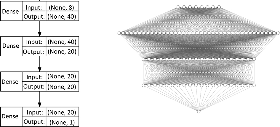
Figure 3. Architecture of the ANNs used in this paper in schematical (Left) and graphical (Right) representation.

We generated all the training data used in the following examples by means of the in-house finite element code BACI (written in C++ and developed at the Institute for Computational Mechanics of the Technical University of Munich, Germany) and a 12-core Intel Xeon E5-2680v3 “Haswell.” In the following, we will skip units, assuming thereby implicitly appropriately normalized quantities. For generating computational models, linear finite element discretizations with variable discretization lengths were used. The error convergence power in (4) is thus assumed to be p = 2 for displacement-based problems as in section “Two-Dimensional Problem: Elastic Deformation of a Thin Membrane Under Loading” and p = 1 for stress/strain-based problems as in section “Three-Dimensional Problem: Elastic Modulus of RVE With Material Inclusion.” The maximal number of epochs within a super-epoch is chosen as E = 100. This number in fact rarely matters and is simply used to ensure that no peculiar situation can arise where the ANN training process can get stuck. The number s of super-epochs for evaluating whether the recent training progress of the ANN has been satisfactory is chosen as s = 3. For the combination of our learning architecture and problem settings, averaging the error over at least the last 3 super-epochs was found to be sufficient to preclude spurious deteriorations of the RMSE from affecting transition points. The number of test samples with maximal fidelity used in (2) and (4) is chosen as $\bar{N}=100$. While this choice is heuristic in nature, it is legitimate because with respect to this number it is only important to keep it high enough to ensure reasonably accurate error estimates and low enough to limit the computational cost for generation of the testing samples compared to the training samples.

Two-Dimensional Problem: Elastic Deformation of a Thin Membrane Under Loading

Problem Description

We consider a square rubber membrane of edge length L = 10. This membrane is modeled as a two-dimensional continuum with pure in-plane extensional and shear stiffness governed by the non-linear neo-Hookean strain energy function

with the material parameter μ = 1 and the (two-dimensional, in-plane) right Cauchy-Green tensor C and its trace tr(C). The membrane forms in its stress-free initial configuration a plane square of edge length L = 10. Before subjecting it to any other loading, it is uniformly stretched in both in –plane directions by a factor of 1.6 and then fixed at all the four edges (zero Dirichlet boundary conditions). Subsequently, the membrane is loaded with four out-of-plane loads. These loads are uniform surface loads of magnitude f = 5 acting on circular domains of radius R = 0.5, respectively. Note that the prestretch by a factor of 1.6 is used here to endow the membrane with a non-zero out-of-plane stiffness at any point in time, which is beneficial for numerically stable computational modeling of the problem.

Our objective is training an ANN to predict the out-of-plane displacement of the center of the membrane, given the (in general variable) positions of the center points of the four surface loads. To this end, we provide the ANN training data where each sample consists of four randomly chosen load positions, which form the input to the ANN, and the associated out-of-plane displacement of the membrane center, which is computed using finite element simulations. For these simulations, we use computational models with n = 5 different levels of fidelity, which correspond to uniform finite element discretizations with $N_{el}^{2d}\in \left\{{10}^2,{20}^2,{40}^2,{80}^2,{160}^2\right\}$ 4-noded rectangular linear membrane elements. Per element the unusually high number of 64 Gauss points were used to evaluate the surface loads on the membrane with an acceptable approximation error even when coarse spatial discretizations are applied. The membrane problem and its discretization with $N_{el}^{2d}=100$ elements are illustrated in Figure 4. In Figure 5 the output of computational models at different fidelity levels (corresponding to 100, 1,600, and 25,400 finite elements) is illustrated for the same input (i.e., same out-of-plane loading).

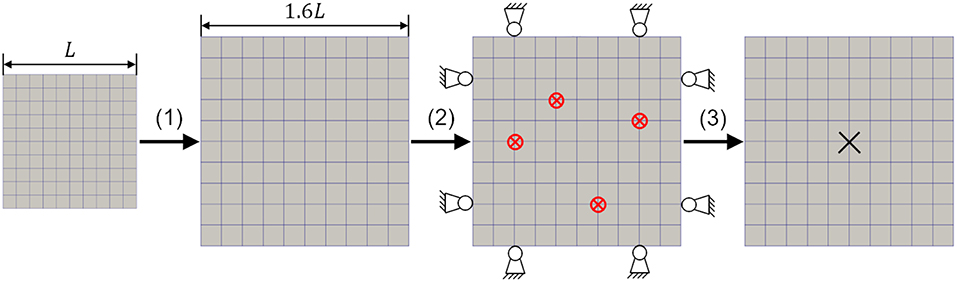
Figure 4. In a computational model with $N_{el}^{2d}=100$ 4-noded membrane finite elements, an initially stress-free elastic rubber membrane is first subjected to an in-plane prestretch by a factor of 1.6 in both directions, then fixed at the boundaries and subjected to out-of-plane loading with circular surface loads (red circles with crosses). Finally, the out-of-plane displacement of the membrane center is recorded in the loaded configuration as output of the computational model. This output forms together with the positions of the four loads a training sample for the ANN with the specific fidelity level corresponding to a discretization with $N_{el}^{2d}=100$ finite elements.

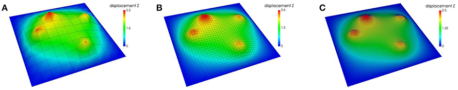
Figure 5. Out-of-plane displacement of membrane subject to certain loading computed with computational models at three different fidelity levels corresponding to (A) 100 elements, (B) 1,600 elements, and (C) 25,600 elements.

Results

We trained an ANN with the architecture from Figure 3 with the three different strategies from section “Different Training Strategies” (single-fidelity, unidirectional multi-fidelity, and bidirectional multi-fidelity) to predict for given positions of the four membrane loads the out-of-plane displacement of the center. Multi-fidelity training required a higher number of samples but was consistently found to reduce the overall computational cost of the training significantly due to the much lower average computational cost of the samples used. Figure 6 and Table 4 report samples numbers, computational cost and learning progress across the different fidelity-levels in case of both single- and multi-fidelity training. In single-fidelity training only samples with highest fidelity (26,500 finite elements) were used for training. It should be noted that the numbers reported are the median over 100 training instances per strategy (reusing generated samples) in order to eliminate the impact of random that is inherent to a training concept were samples are created on the basis of randomly chosen input values. As can be seen in the last column of Table 4, multi-fidelity training enabled us to train the ANN to the same level of accuracy as single-fidelity training at a computational cost that was consistently between a half and one order of magnitude lower. With unidirectional multi-fidelity training computational savings depend on the hyperparameter q in criterion (T2). For sufficiently small choices of q, the criterion (T2) becomes unfulfillable and is functionally removed. Conversely, sufficiently large choices of q lead to a permissive criterion (T2) which will be satisfied whenever it is checked, resulting in fast transitions to the highest fidelity level. In that case, the unidirectional multi-fidelity strategy resembles the standard single-fidelity approach with a minor prefix of a few batches of lower fidelity levels. The best choice of q depends on how accurately equation (4) describes the numerical approximation error, which cannot be easily determined a priori for many problem settings. This heuristic factor is completely eliminated in bidirectional multi-fidelity training where switching between different fidelity levels is performed automatically so as to ensure a computationally efficient training progress. Interestingly, bidirectional multi-fidelity trainings yields this way computational savings that are, at least in this example, comparable to the ones possible with unidirectional multi-fidelity training for favorable choices of q.

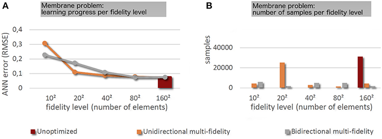
Figure 6. (A) Learning progress across the different fidelity levels for the different training strategies. (B) Number of samples used per fidelity level for the different training strategies.

Table 4. Computation times and sample numbers for different training strategies for the membrane problem from section “Two-dimensional problem: elastic deformation of a thin membrane under loading.”

Three-Dimensional Problem: Elastic Modulus of RVE With Material Inclusion

Problem Description

The second example originates from the field of materials mechanics and is related the broader area of computational homogenization. A classical problem in this area is determining the homogenized (macroscopic) mechanical properties of a material whose microstructure is known in the form of a representative volume element (RVE). The RVEs studied here are cubes with edge length L = 10. They consist of a matrix material into which an ellipsoidal inclusion in the center is embedded. Size and shape of the inclusion are uniquely defined by the three ellipsoidal semiaxes a, b, andc which can vary in a specific prescribed range. Thereby, both the semiaxes and the edges of the RVE are assumed to be aligned with the three coordinate axes x, y, and z. The origin of the coordinate system coincides with the center of the RVE (cf. Figure 7). Both the material of the inclusion and of the surrounding matrix are assumed to be isotropic with Poisson's ratio ν = 0.3. Young's modulus of the matrix is E_m = 1 and of the inclusion E_i = 100. We are interested in computing Young's modulus E_x in x-direction of a material consisting of RVEs of the above described type, depending on the exact geometry of the ellipsoidal inclusion. To this end, one can subject RVEs of the above type to a mechanical loading of the following type: at the face of the RVE oriented in positive x-direction one imposes as a boundary condition a uniform displacement u_x(x = L/2) = 0.05 and at the oppositve face oriented in negative x-direction a uniform displacement u_x(x = −L/2) = −0.05. This mimics an average strain ε_x = 0.01 of the RVE in x-direction. On other faces of the RVE, displacement is constrained such that its component orthogonal to the respective face is uniform across the whole face and that the average outer normal traction vector on each face is zero. Under these conditions, one can compute

(6) with the total reaction force f_x in x-direction on the faces of the RVE oriented in positive and negative x-direction. Our objective is training an ANN to predict E_x, given the (in general variable) lengths a, b, and c of the semiaxes of the ellipsoidal inclusion as input parameters, assuming a, b, c ϵ [2; 4]. To this end, we generate training samples consisting of a random input tuples (a, b, c) and the associated E_x, respectively. The values of E_x are computed by means of finite element simulations of the above described problem. In these simulations, the RVEs are discretized with a uniform mesh of 8-noded hexahedral linear finite elements (Figure 7). We use simulations on four different fidelity levels, corresponding to discretizations with $N_{el}^{3d}=\left\{4^3,8^3,{16}^3,{32}^3\right\}$ elements, respectively (Figure 8).

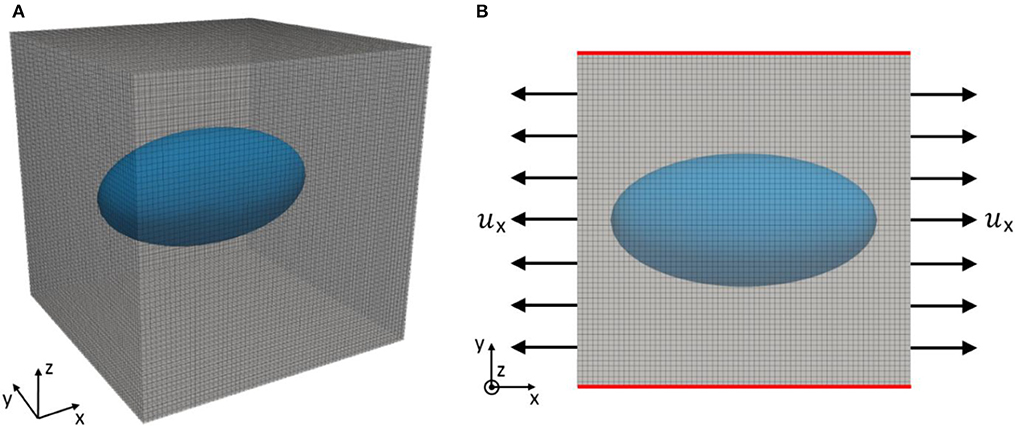
Figure 7. Three-dimensional view (A) and projection onto xy-plane (B) of RVE with ellipsoidal inclusion discretized with $N_{el}^{3d}=262144$ 8-noded hexahedral finite elements. The ellipsoidal inclusion (blue) is located in the center of the RVE and surrounded by a matrix (gray). To probe the stiffness of the RVE in x-direction, a uniform displacement u_x is imposed on the faces in positive and negative x-direction (arrows) while on all the other faces (red) a uniform displacement field perpendicular to the faces with zero average traction in outer-normal direction is imposed.

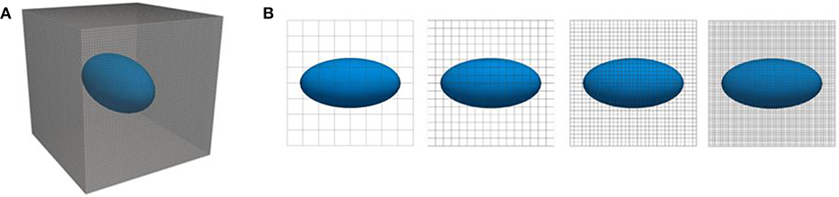
Figure 8. (A) three-dimensional view of RVE with ellipsoidal inclusion, (B) two-dimensional projections of finite elements models of this RVE at four different fidelity levels corresponding to discretizations with a resolution of 4, 8, 16, and 32 elements in each coordinate direction, respectively.

Results

The results for the three-dimensional RVE problem closely resemble the results for the two-dimensional membrane problem presented in the previous “Results” section. The general observation that multi-fidelity strategies require the generation of more samples but yet reduce the total computational cost significantly because the average computation time per sample is much lower is made in two and three dimensions alike. Figure 9 and Table 5 report samples numbers, computational cost, and learning progress across the different fidelity-levels in case of both single- and multi-fidelity training. In single-fidelity training only samples with highest fidelity (262,144 finite elements) were used for training. Again it is noted that the numbers reported here are the median over 100 training instances per strategy for the reasons discussed already in the previous “Results” section. As can be seen in the last column of Table 4, multi-fidelity training enables us to train the ANN to the same level of accuracy at a computational cost that is consistently significantly below the one of single-fidelity training. As one can see, unidirectional multi-fidelity training yields the best results in this three-dimensional example (unlike in the previous two-dimensional example) not for 1 < q < 10 but rather for q < 1 which indicates that the error estimates used for switching between the different fidelity levels may exhibit a considerable inaccuracy. The interaction between the choice of q and the unidirectional multi-fidelity results follows the pattern described in the previous “Results” section. Again one can see that bidirectional multi-fidelity training in which the parameter q is not required and where switching between fidelity levels is performed instead in a smart and automatic way, probing dynamically the computational efficiency of training at different levels of fidelity, is a robust and viable tool to yield an efficiency gain of around half an order of magnitude compared to brute-force single-fidelity training.

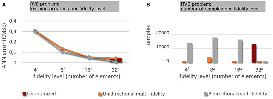
Figure 9. (A) Learning progress across the different fidelity levels for the different training strategies. (B) Number of samples used per fidelity level for the different training strategies.

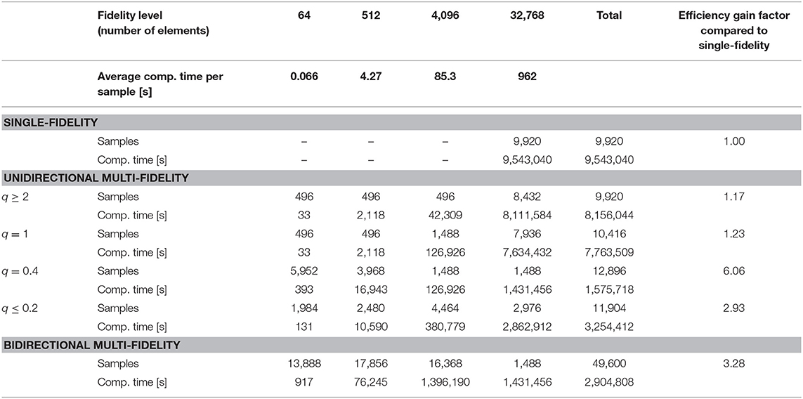
Table 5. Computation times and sample numbers for different training strategies for the membrane problem from section “Two-dimensional problem: elastic deformation of a thin membrane under loading.”

Conclusions

Machine learning and artificial intelligence have attracted rapidly increasing interest in mechanical engineering and materials science over the last years. One of the major challenges in this area is training ANNs to predict or control the behavior of complex physical systems for which not enough real-word training data are available, for example, because experiments or measurements are too expensive, time-consuming, or dangerous. In this case, generating training data by way of realistic computational simulations is a viable and often the only promising alternative. Doing so can, however, be associated with a significant computational cost, which forms a serious bottleneck for the application of machine learning to complex physical systems. To overcome this problem, we propose in this paper a new systematic approach. It exploits the fact that in the initial stage training an ANN mainly aims at endowing the ANN with a coarse understanding of the general features of a problem. Using training data from detailed and thus computationally expensive models can thus be expected to be a waste of computational resources in this stage because coarse low-fidelity models often capture already the most salient features of a physical systems but at much a lower computational cost. Based on this observation, we introduced herein a general and systematic multi-fidelity framework for training ANNs with data generated by computational models with various different fidelity levels. Such models can easily be generated in the context of widely used computational methods such as the finite element method by varying the discretization length. In this framework, cheap low-fidelity computational models are used to generate the training data for the early stages of ANN training. As the training of the ANNs progresses, one gradually switches to higher-fidelity training data generated by means of more accurate and computationally more expensive models. This strategy is very general in nature and can in principle be applied to any problem where training ANNs computational models are used whose accuracy can straightforwardly be controlled, for example, by way of a discretization length. This is true not only for the finite element method which we are using herein but also for numerous other methods for solving partial differential equations such as finite difference methods, mesh-free discretization schemes such as the moving least squares methods or particle-based methods such as smoothed particle hydrodynamics (SPH). In this article, we focused on two application areas, which are structural mechanics and materials mechanics. In these areas computational models are already widely used and coupling them with machine learning appears the natural next step to address several key problems such as efficient prediction of the behavior of complex mechanical systems under variable (e.g., loading) conditions or efficient homogenization of the mechanical behavior of complex materials with a heterogeneous microstructure depending on certain features of this microstructure.

We developed in this article a general multi-fidelity framework and discussed two slightly different versions of it. The first one is based on an estimate of the error of the computational models used at different fidelity levels. It implies a heuristic correction factor q. While it may often be possible to determine this correction factor based on simple rules of thumb, in other cases this may be more difficult. This dependency on q, which does not straightforwardly generalize to complex hybrid models (e.g., finite elements on one level, molecular dynamics on another level, other discretization schemes) is a drawback of the unidirectional multi-fidelity variant, which furthermore has the limitation of no clear method of a priori calculating the most efficient transition points between levels of fidelity. To eliminate this heuristic element and the problems it entails, we proposed a second version of our multi-fidelity framework where switching between different fidelity levels is controlled in a smart and fully automated way. To this end, our training algorithms probes at each fidelity level training samples also from neighboring fidelity levels and dynamically switches to the fidelity level where currently the largest training progress per computational cost can be achieved. We would consider this method a robust variant of the multi-fidelity strategy, relying on fewer parameters than the unidirectional approach. In summary, we found that our multi-fidelity training strategy enables us to train ANNs to the same level of accuracy as standard (single-fidelity) approaches but at a computational cost that is by around a half to one order of magnitude lower. This gives rise to the hope that the general multi-fidelity strategy introduced herein can become a powerful and versatile tool for the future combination of computational simulations and artificial intelligence, in particular in the area of structural and materials mechanics.

We conclude this paper by noting that the two specific multi-fidelity training algorithms introduced in this paper, the unidirectional and the bidirectional training algorithm, are but a starting point. There are various ways how the underlying general idea of systematic multi-fidelity training can be further developed and optimized. For example, one could employ for ANN training batches where samples with several different fidelity levels are mixed. This would enable a seamless transition between different fidelity levels during training, which might yield additional computational savings.

Author Contributions

RA and CC conceived of the presented approach and developed and employed the machine learning model. FB developed and performed the computational examples. RA wrote the main part and assembled all of the manuscript. All authors discussed the results and contributed to the final manuscript.

Conflict of Interest Statement

The authors declare that the research was conducted in the absence of any commercial or financial relationships that could be construed as a potential conflict of interest.

Acknowledgments

Funded by the Deutsche Forschungsgemeinschaft (DFG, German Research Foundation) − Projektnummer 192346071 − SFB 986; Projektnummer 257981274.

References

Abadi, M., Barham, P., Chen, J., Chen, Z., Davis, A., Dean, J., et al. (2016). “Tensorflow: A System for Large-Scale Machine Learning,” in OSDI'16 Proceedings of the 12th USENIX conference on Operating Systems Design and Implementation. (Savannah, GA: Osdi), 265–283.
Domingos, P. (2012). A few useful things to know about machine learning. Commun. ACM 55, 78–87. doi: 10.1145/2347736.2347755
Hu, Y., Xie, J., Liu, Z., Ding, Q., Zhu, W., Zhang, J., et al. (2018). CA method with machine learning for simulating the grain and pore growth of aluminum alloys. Comput. Mater. Sci. 142, 244–254. doi: 10.1016/j.commatsci.2017.09.059
Kingma, D., and Ba, J. (2015). “Adam: A Method for Stochastic Optimization,” in Proceedings of the 3rd International Conference on Learning Representations (ICLR 2015). arXiv[Preprint].arXiv:1412.6980.
Mosallam, A., Medjaher, K., and Zerhouni, N. (2016). Data-driven prognostic method based on Bayesian approaches for direct remaining useful life prediction. J. Intell. Manuf. 27, 1037–1048. doi: 10.1007/s10845-014-0933-4
Pilania, G., Gubernatis, J. E, and Lookman, T. (2017). Multi-fidelity machine learning models for accurate bandgap predictions of solids. Comput. Materi. Sci. 129, 156–163. doi: 10.1016/j.commatsci.2016.12.004
Russell, S. J., and Norvig, P. (2016). Artificial Intelligence: A Modern Approach. Malaysia: Pearson Education Limited.
Silver, D., Huang, A., Maddison, C. J, Guez, A., Sifre, L., van den Driessche, G., et al. (2016). Mastering the game of Go with deep neural networks and tree search. Nature 529, 484–489. doi: 10.1038/nature16961
Silver, D., Schrittwieser, J., Simonyan, K., Antonoglou, I., Huang, A., Guez, A., et al. (2017). Mastering the game of go without human knowledge. Nature 550, 354–359. doi: 10.1038/nature24270
Vinyals, O., Ewalds, T., Bartunov, S., Georgiev, P., Sasha Vezhnevets, A., Yeo, M., et al. (2017). StarCraft II: a new challenge for reinforcement learning. arXiv[Preprint].arXiv:1708.04782.
Wang, H., Zhang, W., Sun, F., and Zhang, W. (2017). A comparison study of machine learning based algorithms for fatigue crack growth calculation. Materials 10:E543. doi: 10.3390/ma10050543
Waszczyszyn, Z., and Ziemianski, L. (2001). Neural networks in mechanics of structures and materials–new results and prospects of applications. Comput. Struct. 79, 2261–2276. doi: 10.1016/S0045-7949(01)00083-9
Keywords: artificial intelligence, homogenization, material science, machine learning, simulation
Citation: Aydin RC, Braeu FA and Cyron CJ (2019) General Multi-Fidelity Framework for Training Artificial Neural Networks With Computational Models. Front. Mater. 6:61. doi: 10.3389/fmats.2019.00061
Received: 04 February 2019; Accepted: 25 March 2019;
Published: 17 April 2019.
Edited by:
Roberto Brighenti, University of Parma, ItalyReviewed by:
Ercan Gürses, Middle East Technical University, TurkeyYouyong Li, Soochow University, China
Copyright © 2019 Aydin, Braeu and Cyron. This is an open-access article distributed under the terms of the Creative Commons Attribution License (CC BY). The use, distribution or reproduction in other forums is permitted, provided the original author(s) and the copyright owner(s) are credited and that the original publication in this journal is cited, in accordance with accepted academic practice. No use, distribution or reproduction is permitted which does not comply with these terms.
*Correspondence: Roland Can Aydin, roland.aydin@hzg.de