Influence of tidal mixing on bottom circulation in the Caroline Sea

1 Introduction

Meridional overturning circulation (MOC) plays a crucial role in sustaining the global transport of water, heat and substances (e.g., Talley, 2013), and its variability may affect the regional climate change in global warming period (e.g., Zhao et al., 2023). The upwelling of the relatively cold and saline deep water that occurred in the tropical Pacific Ocean is an important component of the global MOC. The Caroline Sea is located in the tropical western Pacific Ocean, with two semi-enclosed abyssal basins, namely the West Caroline Basin (WCB) and the East Caroline Basin (ECB). Below 4000 m depth, the WCB and ECB are isolated without direct water exchange with surrounding oceans. Yet, the bottom water in the East Mariana Basin (EMB), mainly composed of the Lower Circumpolar Deep Water (LCDW; Kawabe and Fujio, 2010), can flow into the WCB by passing through the Yap Trench (YT; Kaneko et al., 1998) and enter the ECB via the channel near the East Fayu (hereinafter referred to as EFC; Siedler et al., 2004). Thus, net upwelling must occur in the bottom water of the two basins to compensate the overflow. Kawabe and Fujio (2010) speculated that about 2 Sv (1 Sv = 10⁶ m³ s^-1) of LCDW upwells into the upper deep layer and ultimately into the surface/intermediate layer in the WCB and ECB, which contributes about one third of the total water (6 Sv) upwelling into the surface/intermediate layer in the North Pacific. It is therefore essential to investigate the bottom water and circulation as well as the potential thermodynamics mechanism in the Caroline Sea for better understanding of the global MOC.

However, there have been only limited studies on the bottom layer of the Caroline Sea over the past several decades, which were mainly based on quite sparse observations. Using the full-depth high-resolution hydrographic measurements along the WHP-P9 section (137°–142°E), Kaneko et al. (1998) showed that the bottom water properties over the YT and in the WCB were almost the same as that in the southern West Mariana Basin (WMB), and suspected that a part of EMB bottom water entered the WCB via the YT with a transport estimated to be 0.5–1.0 Sv. Kawabe et al. (2003) used several CTDO2 section observations to describe the near-bottom layers water in the ECB at 150°E and the WCB at 140°E, which were much warmer, fresher and less oxygenated than that in the WMB. By both geostrophic flow calculations and independent sill current measurements, Siedler et al. (2004) confirmed that the LCDW could enter not only the WMB but also the ECB, and obtained a geostrophic transport of 0.45 Sv below 4000 m at the EFC. Kawabe and Fujio (2010) proposed that the total LCDW inflow to the WCB and ECB was speculated to be about 2 Sv based on the diagnostic calculations from hydrographic data. The observations in the YT by Liu et al. (2018; 2020; 2022) indicated a northward geostrophic deep flow over the sill between the southern and northern trench, a southward (northward) flow in the western (eastern) region of the southern trench, and a southward overall transport. By analyzing the historical measurements from the World Ocean Database 2018, Germineaud et al. (2021) also showed the evidence for the existence of the LCDW in the ECB below 4000 m. Due to the difficulty of observation in the deep and bottom water, there is still a huge lack of sufficient observational hydrographic and current data in the bottom layer of Caroline Sea, thus the amount of water inflow and the detailed distributions of water properties and circulation in the abyssal WCB and ECB remain largely unclear.

Diapycnal mixing is thought to be one of the most important controlling factors of the global ocean stratification and MOC (Marshall and Speer, 2012; Talley, 2013). One of the energy sources for diapycnal mixing is the internal tides generated by the interaction of barotropic tides with rough seafloor topography, with a global energy conversion of about 1 TW in the deep ocean (Egbert and Ray, 2000; Jayne and St. Laurent, 2001; Niwa and Hibiya, 2014), which contributes about half of the total (2 TW) required to sustain the global MOC (Munk and Wunsch, 1998). The WCB and ECB are surrounded by numerous submarine ridges and seamounts, where energetic internal tides are generated (Niwa and Hibiya, 2001; Buijsman et al., 2017). Part of the internal tides would be dissipated locally near the generation sites, and the other part would propagate away and be dissipated somewhere else, including the WCB and ECB (Niwa and Hibiya, 2011; Zhao et al., 2016). Therefore, it is speculated that tidal mixing (diapycnal mixing induced by internal tides dissipation) could be an essential driving force for the bottom water transformation and overturning circulation in both the WCB and the ECB. However, the observations and estimates of diapycnal/tidal mixing in the two basins were hardly reported. Siedler et al. (2004) estimated the diapycnal mixing that is required to balance the LCDW inflow to the ECB as the order of O(10^-3) m² s^-1. Some important issues remain unclear, such as how the three-dimensional spatial distribution of tidal mixing exhibits in the Caroline Sea, to what extent tidal mixing could influence the bottom water exchange between the basins, and whether tidal mixing contributes to the basin/subbasin-scale distributions of bottom water and circulation within the basins.

In this study, we will construct a regional ocean model, and carry out a series of numerical experiments by employing different diapycnal diffusivities of tidal mixing. The vertical resolution of our model is not fine enough to directly simulate diapycnal mixing induced by internal wave breaking. Thus, even if the barotropic tide is set as the direct driving force in the model, the tidal dissipation and mixing processes still cannot be actually resolved. Therefore, the parameterization of diapycnal diffusivities is needed in the model to represent the mixing processes more accurately. Moreover, because the abyssal observations available for model validation are rather sparse and the impacts of diapycnal mixing on simulation biases would depend largely on individual model configuration (Melet et al., 2013), we will not focus on the possible improvements of the model in this study. Instead, the sensitivity of the ocean state to tidal mixing are not expected to be model dependent. Thus, the purpose of this paper is to investigate the influence of tidal mixing on the bottom water properties and circulation in the Caroline Sea, as well as the potential dynamic mechanisms.

This paper is organized as follows: The estimate of tidal mixing and the configuration of regional ocean model are introduced in Section 2. The results of the numerical experiments are presented and analyzed in Section 3. Finally, summary and discussion are given in Section 4.

2 Methods

2.1 Tidal mixing estimate

Diapycnal diffusivities of tidal mixing are estimated by two methods with the same horizontal and vertical resolution in this study. One method is a semi-empirical parameterization scheme proposed by St. Laurent et al. (2002, hereinafter referred to as LSJ02):

This scheme first calculates the two-dimensional internal tides energy flux E (Jayne and St. Laurent, 2001):

Where ${\rho }_0$ is the reference density, $N_b$ is the buoyancy frequency at the seafloor, and both are calculated from the World Ocean Atlas 2013 version 2 (WOA13v2, Locarnini et al., 2013; Zweng et al., 2013). k is the wavenumber scale of the seafloor topographic roughness, set as a spatial constant of 2π/(5 km) throughout the domain. h² is the amplitude scale of the seafloor topographic roughness, which is computed as the mean-square of height deviations from a polynomial sloping surface fit of the seafloor topography to a plane over a grid box, using the high resolution (1/120°) bathymetry data of the Gridded Bathymetric Chart of the Oceans (GEBCO) (http://www.gebco.net/). $\langle u_{bt}^2\rangle$ is the tidal-period mean of squared barotropic tidal speed computed from the results of our internal tide model introduced below. Then, a local dissipation efficiency q = 0.3 is set according to the LSJ02, to obtain the portion that dissipated near the generation sites of internal tide.

After that, to obtain a three-dimensional distribution that satisfies energy conservation within an integrated vertical column, a vertical structure function $F(z)$ is adopted,

which assumes that local tidal dissipation are bottom intensified and exponentially decay away from the seafloor with a vertical e-folding decay scale ζ = 500 m and the total depth of water column D. Finally, the three-dimensional field of diapycnal diffusivities κ is derived by use of the relation of Osborn (1980), with the mixing efficiency Γ= 0.2, seawater density ρ, squared buoyancy frequency N², and a background diffusivity κ_{0 =} 1×10^-5m² s^-1. Refer to St. Laurent et al. (2002) for detailed descriptions of this method. The LSJ02 scheme only takes into account the local part of tidal dissipation, while ignores the part that propagates and dissipates away from the generation sites.

The other method follows the work of Wang et al. (2016). Firstly, a three-dimensional high-resolution internal tide model is constructed to simulate the generation and propagation of internal tides. The model is based on the Massachusetts Institute of Technology General Circulation Model (MITgcm; Marshall et al., 1997), and its domain extends from 112°E to 165°E and from 25°S to 45°N, covering the entire of the Philippine Sea, the Indonesian Archipelago, the Caroline Sea and the EMB, as well as part of the northwest Pacific Basin (Figure 1A). The horizontal resolution is 1/20°×1/20°, and the vertical layers are 82 z-levels with the thickness of layers gradually increased from 5 m near surface to 200 m above the bottom. The model is initialized with horizontally homogeneous and vertically stratified temperature and salinity fields obtained from the WOA13v2 data, and forced by four primary tidal constituents (M₂, S₂, K₁, and O₁) at the open boundaries. Then, using the output of internal tide model, the depth-integrated barotropic-to-baroclinic energy conversion $E_{bt2bc}$ and the divergence of depth-integrated baroclinic energy flux ${\nabla }_h·F_{bc}$ are calculated. Assuming the tidal-period mean of internal energy density is constant at a fixed area and neglecting the advection of internal energy, the tidal-period mean of depth-integrated dissipation rate can be approximately estimated as:

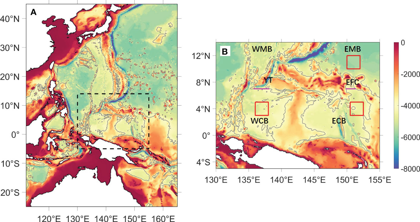
Figure 1 (A) Bathymetry (unit: m) of the model domain, and (B) zoomed‐in bathymetry (unit: m) of the Caroline Sea in the black dashed box in (A). Three red boxes in (B) indicate the regions used to calculate area-averaged potential density profiles, including the EMB (150°-152°E, 10°-12°N), WCB (136°-138°E, 3°-5°N) and ECB (150.5°-152.5°E, 3°-5°N), respectively. Two magenta lines in (B) represent the sections used to calculate water flux between upstream regions and the WCB/ECB, respectively. The grey contours represent the 4000-m isobaths. WMB, West Mariana Basin; EMB, East Mariana Basin; WCB, West Caroline Basin; ECB, East Caroline Basin; YT, Yap Trench; EFC, East Fayu Channel.

Finally, the three-dimensional field of diapycnal diffusivities is obtained by assuming the same vertical decay structure as in the LSJ02 scheme and the Osborn (1980) relation. Refer to Wang et al. (2016) for detailed descriptions of this method. Based on the internal tide simulation and the energy budget analysis (hereinafter referred to as ITSEBA), the total (both local and remote) tidal dissipation are taken into account in this method. Therefore, its estimates are relatively closer to the actual situation and thus more accurate for representing tidal mixing distributions, especially in abyssal basins where the energy of internal tides are mainly propagated from the surrounding rough topography. Note that in this study, the remote tidal dissipation/mixing at one site refers to the contribution from the internal tides which are generated at other far-field sites and finally broken to turbulence at this site, rather than the internal tides generated at this site and propagated away.

In this study, we will focus on the region of Caroline Sea and its surroundings (Figure 1B). Depth-integrated dissipation of internal tides is shown in Figure 2. The estimate from the LSJ02 scheme (Figure 2A) shows that the strong local dissipation mainly concentrates at some patches atop islands, submarine ridges and seamounts, with magnitude reaching O(10^-2–10^-1) W m^-2; yet besides which, the local dissipation elsewhere is much weaker, with magnitude of O(10^-4–10^-3) W m^-2 near ridges and above the Eauripik Rise, as well as O(10^-6–10^-5) W m^-2 within the abyssal basins. The estimate from the ITSEBA method (Figure 2B) exhibits a significantly different pattern. Strong dissipation occurs extensively above submarine ridges and seamounts with dissipation rate of O(10^-2) W m^-2, while the dissipation within the abyssal basins is relatively weaker with magnitude of about O(10^-3) W m^-2. In general, the estimate from the ITSEBA method is one to three orders of magnitude stronger than that from the LSJ02 scheme. These discrepancies are due to the different tidal dissipation processes taken into account in these two methods.

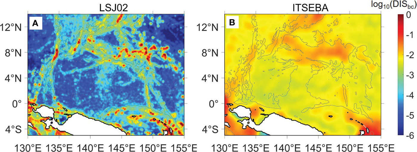
Figure 2 Depth-integrated dissipation (unit: W m^-2) of internal tides estimated from (A) the LSJ02 scheme and (B) the ITSEBA method, respectively. The grey contours represent the 4000-m isobath.

Abyssal diapycnal diffusivities estimated from the two methods also show enormous differences on distribution patterns and magnitude (Figure 3). In the LSJ02 scheme (Figures 3A, C, E), strongest tidal mixing occurs only within some local narrow water columns, with magnitude of O(10^-5–10^-4) m² s^-1. Mixing in the ECB is much stronger than that in the WCB (Figure 3A), due to the much rougher bottom topography and hence more local dissipation occurred in the ECB. However, in the ITSEBA method (Figures 3B, D, F), strongest tidal mixing occurs throughout the bottom water of the two basins, as well as the two deep-water passages of YT and EFC. The elevated diapycnal diffusivity is about O(10^-3–10^-2) m² s^-1, and the thickness of bottom water exceeding O(10^-3) m² s^-1 could reach 1000 m above the bottom. Compared to the estimate of LSJ02 scheme, the diapycnal diffusivities obtained from the ITSEBA method are increased not only in the deep basins of the Caroline Sea but also over the marine ridges and seamounts. The remotely-generated internal tides could impose a great impact on tidal mixing processes by multiple ways concurrently, such as providing enormous baroclinic tidal energy; modifying the local barotropic-to-baroclinic energy conversion, and interacting with the locally-generated internal tides (Wang et al., 2016). Tidal mixing estimated from the ITSEBA method is generally one to three orders of magnitude stronger than that from the LSJ02 scheme, and is more consistent with the estimate by Siedler et al. (2004).

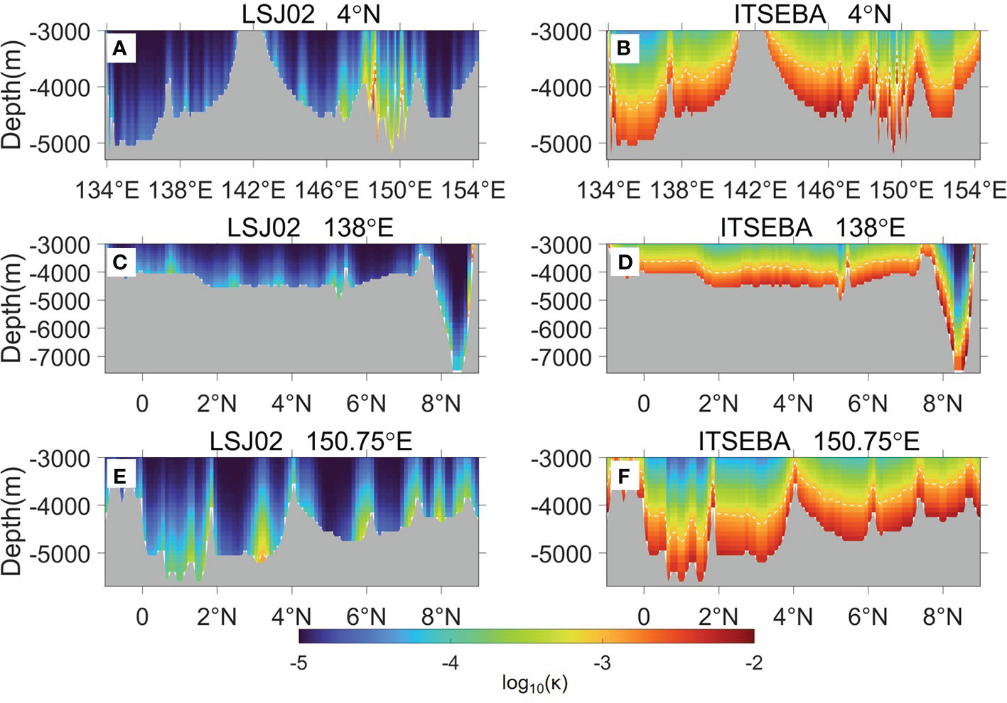
Figure 3 Cross-sectional distributions of diapycnal diffusivity (unit: m² s^-1) along (A, B) 4°N, (C, D) 138°E and (E, F) 150.75°E in the Caroline Sea, estimated from (A, C, E) the LSJ02 scheme and (B, D, F) the ITSEBA method, respectively. The white dashed lines represent contours of 1×10^-3 m² s^-1.

2.2 Regional model configuration

A high resolution regional circulation model of the western Pacific Ocean is constructed based on the MITgcm, and the model domain is the same as the internal tide model (Figure 1A). The horizontal resolution is 1/10°×1/10°, and the vertical layers are the same as the internal tide model. Model bathymetry is obtained from the high resolution (1/120°) GEBCO data (http://www.gebco.net/). The initial temperature and salinity fields are monthly mean of January derived from the WOA13v2. The surface forcing of climatological monthly mean wind stress is calculated from the Cross-Calibrated Multiplatform (CCMP) datasets (Atlas et al., 2011). At the four open boundaries, the climatological monthly mean of potential temperature, salinity, as well as zonal and meridional velocities from the SODA version 2.2.4 (https://climatedataguide.ucar.edu/climate-data/soda-simple-ocean-data-assimilation) are applied, which is also used as the relaxations of sea surface temperature and salinity.

The horizontal viscosity coefficients are calculated with the Smagorinsky (1993) scheme, and the isopycnal diffusivity coefficients are set to be 500 m² s^-1. To eliminate spurious diapycnal mixing introduced by advection schemes, the Gent–McWilliams/Redi (GMRedi) subgrid-scale eddy parameterization (Redi, 1982; Gent and McWilliams, 1990; Gent et al., 1995) is adopted. The vertical viscosity coefficients and a portion of vertical diffusivity coefficients are calculated by the KPP scheme (Large et al., 1994), and the diapycnal diffusivities related to tidal mixing as estimated in section 2.1 are also added in the model. Three experiments are designed based on different tidal mixing configurations. The experiment NoTM only uses the KPP scheme with a uniform background diffusivity of 1×10^-5 m² s^-1, that is, completely without consideration of tidal mixing. In experiment LSJ, diapycnal diffusivities calculated by the LSJ02 scheme are added, that is, only the local tidal mixing is considered. In experiment TM, diapycnal diffusivities estimated by the ITSEBA method are adopted, in which tidal mixing processes induced by the total dissipated tidal energy are taken into account.

All experiments start from rest and are integrated for 400 years. The total kinetic energy of all experiments at both the upper and deep layers reached quasi-equilibrium by the end of the 400-year simulation. In this study, we will focus on the results of Caroline Sea and its surroundings, and the average of model output in the last 10 model years are used for analysis.

3 Results

3.1 Bottom water properties

The potential density σ₄ at 4000 m depth of the Caroline Sea is exhibited in Figure 4. The water properties are quite homogeneous both in NoTM (Figure 4A) and LSJ (Figure 4B), with σ₄ of 45.860–45.862 kg m^-3. In NoTM, σ₄ of the WCB is a little lower than that of the ECB, and the contrary happens in LSJ. However in TM (Figure 4C), water properties are quite inhomogeneous both in the ECB and WCB, with the highest σ₄ exceeding 45.855 kg m^-3 near the north entrances and the lowest σ₄ less than 45.840 kg m^-3 along boundaries or at corners of both basins. The horizontal gradient of σ₄ in TM is much higher than that in NoTM and LSJ, and gradually decreases from the entrance toward the interior of basins.

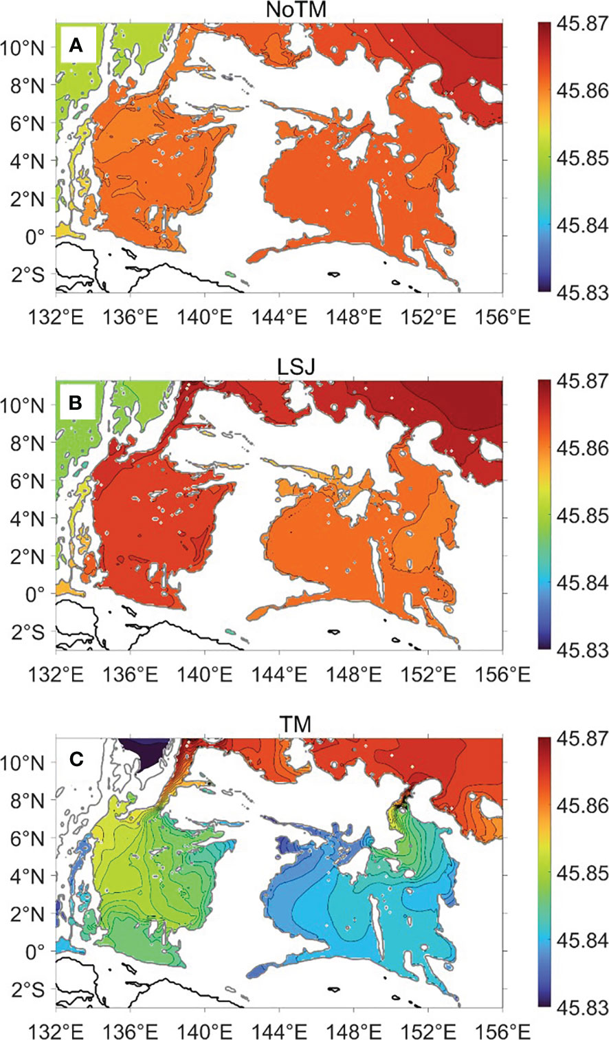
Figure 4 Potential density σ₄ (unit: kg m^-3) at 4000 m of the Caroline Sea in the experiments (A) NoTM, (B) LSJ and (C) TM, respectively. The black contours intervals are 0.001 kg m^-3. The grey contours represent the 4000-m isobaths.

To further examine the effect of tidal mixing on the deep water properties of the Caroline Sea, differences of potential temperature (Δθ) and salinity (ΔS) between LSJ/TM and NoTM are demonstrated through the cross-sectional distributions along 4°N in Figure 5 and the basin-averaged profiles in Figure 6. The Δθ and ΔS between LSJ and NoTM (Figures 5A, C) are both quite small in the two basins, with the basin-averaged differences less than ±0.02°C and ±0.002 psu (Figure 6), respectively. However, differences between TM and NoTM (Figures 5B, D) are distributed unevenly and significant, with a basin-averaged temperature increase of about 0.02–0.85°C and salinity decrease of 0.005–0.012 psu (Figure 6), respectively. In TM, the bottom water becomes warmer and fresher over the whole two basins, and relatively larger changes appear above the seafloor where the diapycnal diffusivities are also relatively higher (Figure 3B).

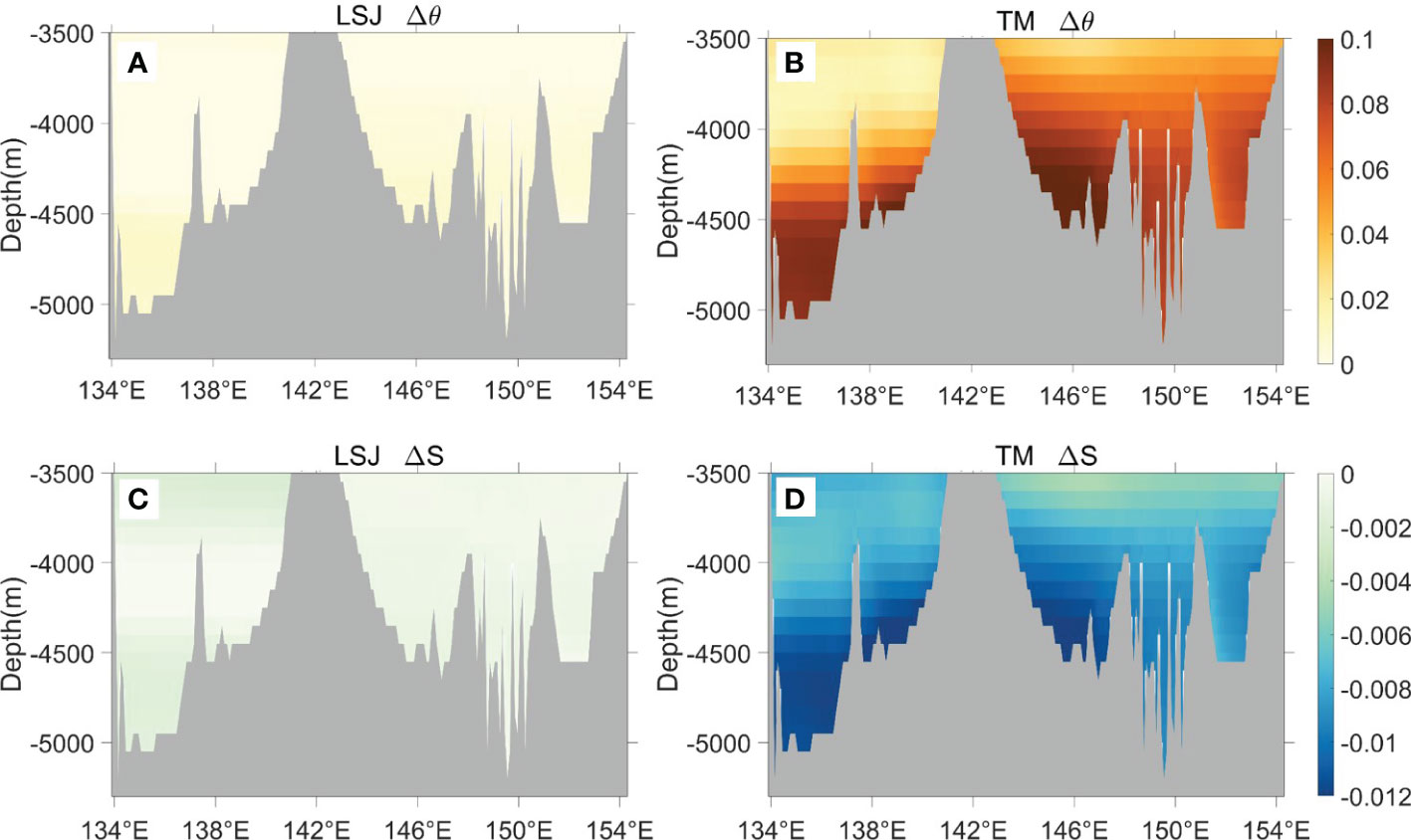
Figure 5 Cross-sectional distributions along 4°N of the differences in potential temperature (Δθ, unit:°C) and salinity (ΔS, unit: psu) between (A, C) LSJ and NoTM, as well as between (B, D) TM and NoTM.

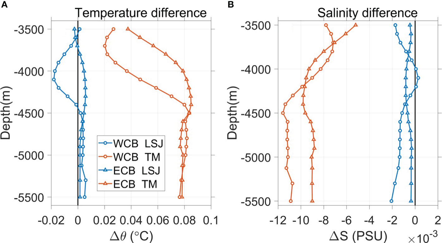
Figure 6 Basin-averaged differences of (A) potential temperature (Δθ) and (B) salinity (ΔS) between LSJ/TM and NoTM, in the WCB and ECB, respectively.

In the abyss of WCB and ECB, the local tidal mixing is weak (Figure 3A), thus has rather little impact on the bottom water properties of the Caroline Sea as in LSJ. In contrast, the abyssal diapycnal mixing in the two basins is significantly enhanced by the total tidal dissipation (Figure 3B). Under large diapycnal diffusivities in TM, the simulated LCDW first gets strongly mixed with the overlying relatively warmer and fresher water while flowing through the YT and EFC, respectively, which results in the much lighter water intrusion into the abyssal WCB and ECB than in other two experiments. Then, the modified LCDW continuously experiences elevated diapycnal mixing while spreading throughout the basins, so that the horizontal gradients of potential density are strengthened and sustained (Figure 4C). These results suggest that tidal mixing processes could extremely enhance the bottom water transformation in the WCB and ECB at the basin scale.

3.2 Bottom water transport

At the entrances of the WCB and ECB along 7°N, one section near the YT and the other one near the EFC (Figure 1B) are used to explore the water exchange between the upstream regions and the two basins, respectively. The evolutions of water fluxes below 4000m in three experiments are shown in Figure 7, in which the positive (negative) value represents the outflow (inflow) for the WCB and ECB. In NoTM and LSJ, the bottom water fluxes are initially southward into the WCB through the YT (Figure 7A), and decrease gradually from the start of spin-up. A quasi-equilibrium inflow of about 0.02 Sv is obtained in LSJ, while in NoTM the water flux finally decreases from southward to an opposite direction of northward and thus becomes an outflow from the WCB of about 0.01 Sv. In contrast, the bottom water flux in TM increases rapidly during the first ~30 model years and finally achieves a quasi-equilibrium inflow at about 0.82 Sv. The comparisons of the transport among three experiments for the ECB (Figure 7B) are similar to that for the WCB (Figure 7A). The quasi-equilibrium bottom water inflow through the EFC into the ECB obtained in NoTM, LSJ and TM are about 0.09 Sv, 0.17 Sv and 1.02 Sv, respectively. Generally, the bottom water transports obtained in experiment TM are consistent with previous studies. The inflow to WCB in TM (0.82 Sv) is close to the upper bound (1.0 Sv) of Kaneko et al. (1998), both of which were calculated at sections of the same latitude (7°N). The inflow to ECB in TM (1.02 Sv) is more than twice that (0.45 Sv) of Siedler et al. (2004), the latter of which was calculated at a further north positon of 8°40′N. The total transport into two basins is 1.84 Sv in TM, which is quite close to the estimate of 2.0 Sv by Kawabe and Fujio (2010). In contrast, the bottom water transports in experiments NoTM and LSJ are seriously underestimated in comparison with previous studies, which are one order of magnitude and more than 40% weaker for the YT and the EFC, respectively.

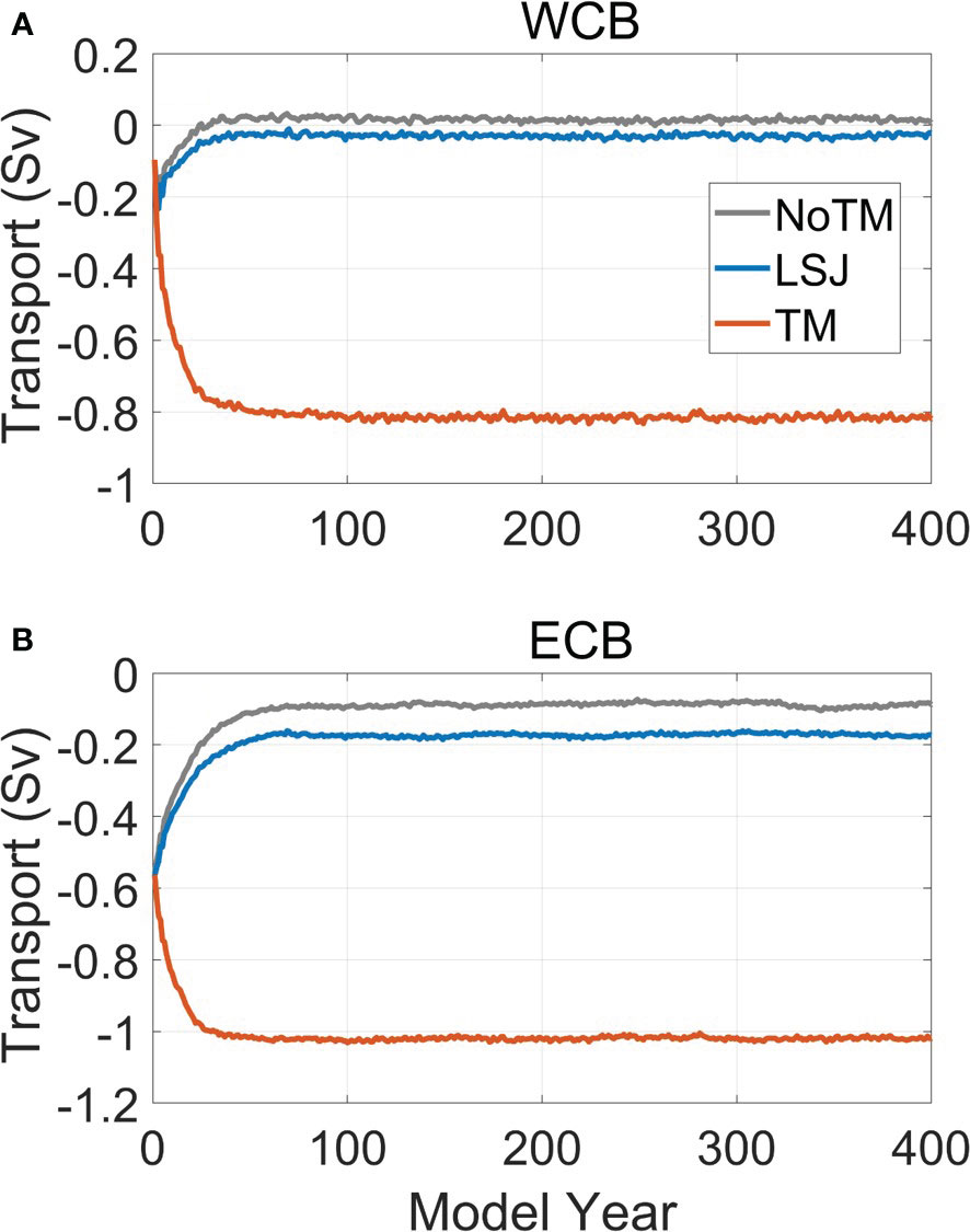
Figure 7 Time evolutions of water flux (unit: Sv) below 4000 m between upstream regions and the two basins, respectively: (A) WCB; (B) ECB.

To further explain the impact of tidal mixing processes on the bottom water transport, the differences of σ₄ between the EMB and WCB (Figure 8A), as well as that between the EMB and ECB (Figure 8B) are illustrated with area-averaged profiles (The results are not sensitive in qualitative to the selection of areas, not shown). In NoTM and LSJ, either without tidal mixing or only with weak local tidal mixing, the gradient of σ₄ and thus that of the horizontal pressure between the EMB and WCB/ECB cannot be sustained. In this circumstance, the bottom water transport into WCB/ECB cannot be driven continuously and thus decreases gradually. As a result, after sufficient long model integration, the bottom water fluxes finally reach a rather small inflow or even outflow state in NoTM and LSJ. In contrast, the bottom water transport in TM can reach a quasi-equilibrium state with a much higher magnitude. This is because that with the elevated tidal mixing in both the YT (EFC) and WCB (ECB), the consistent watermass transformation and hence the required horizontal pressure gradient force can be maintained. These results of our experiments reveal that tidal mixing processes play key roles in sustaining the bottom water transport into the abyssal WCB and ECB.

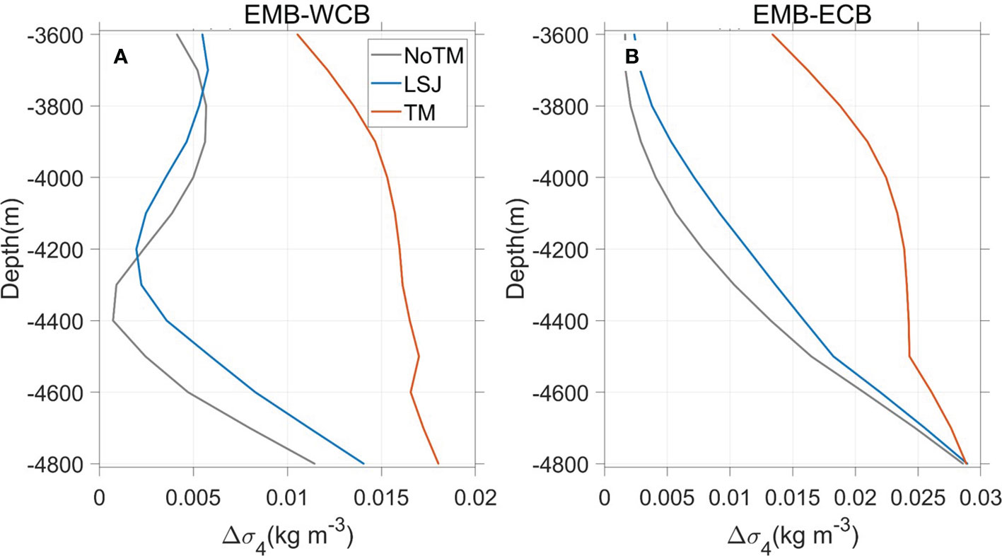
Figure 8 Area-averaged profiles of potential density differences $△{\sigma }_4$ between (A) the EMB and WCB, as well as (B) the EMB and ECB in different experiments. The areas are marked with three red boxes in Figure 1B.

3.3 Bottom circulation

The vertically averaged horizontal currents below 4000 m in the Caroline Sea in three numerical experiments are shown in Figure 9. In NoTM (Figure 9A) and LSJ (Figure 9B), bottom circulations are extremely weak in the whole two basins, as a result of the rather weak horizontal density gradients within basins (Figures 4A, B). In contrast, the simulated bottom circulation in TM is much stronger (Figure 9C) with complex subbasin-scale structures. After entering the WCB through the YT, the current bifurcates into two branches, one is an eastward flow, and the other flows southward along the western boundary. The latter turns eastward at the central of the basin, and bifurcates into two branches again, among which one continues eastward and turns southward at the eastern boundary, while the other turns southward and then westward to become a western boundary current in the southernmost region. In the ECB, a strong southward inflow is injected into the eastern subbasin via the EFC, and then turns westward across the central gap into the western subbasin. Then current bifurcates into a westward and a southward branches, which finally joint to form a strong western boundary current in the western subbasin. These results of our experiments reveal that tidal mixing processes could extremely strengthen the basin/subasin-scale bottom circulation and in the Caroline Sea. The bottom topography should also play a role in the formation of the subbasin-scale bottom circulation. However, in three experiments, the bottom topography is all the same, while the distributions of vertical diffusivity are different. Thus, the subbasin-scale distribution of bottom intensified tidal mixing probably plays a key role in driving the higher speed and the more complex subbasin-scale structure of the bottom circulation.

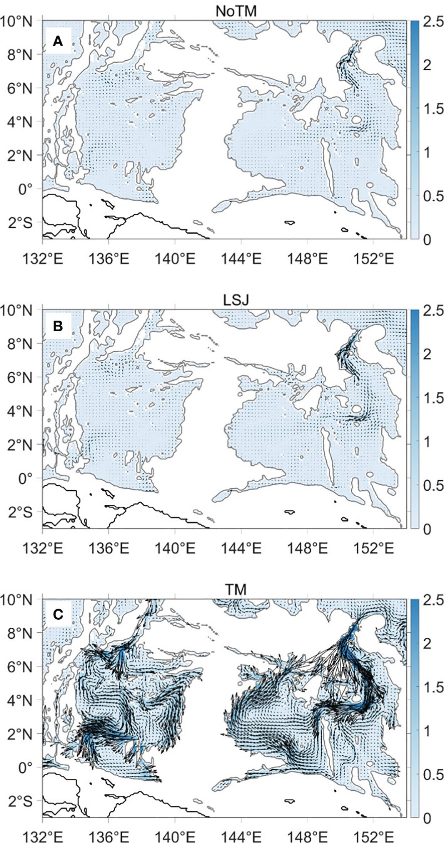
Figure 9 Vertical-averaged currents (unit: cm s^-1) below 4000 m in experiments (A) NoTM, (B) LSJ and (C) TM, respectively. The grey contours represent the 4000-m isobaths.

The WCB and ECB are closed below 4000 m, thus the meridional streamfunction $\Psi (y,z)$ could be calculated to examine the bottom MOC in the two basins, which is defined as

where v is the meridional component of velocity, and x_e and x_w are the locations of the eastern and western boundaries respectively. Positive and negative streamlines indicate the counterclockwise and clockwise circulations, respectively. The bottom meridional streamfunction of the WCB and ECB in NoTM and LSJ are all extremely weak (Figures 10A–D), and structures of streamfunction in the same basin are quite similar between NoTM and LSJ. In contrast, the bottom meridional streamfunction in TM are clockwise and intensely enhanced in both the two basins. In the WCB (Figure 10E), the water inflows around 4000 m via the YT, then falls into the northern region of the abyssal basin and transports southward, and eventually upwells in the southern abyssal basin. In the ECB (Figure 10F), the water inflows to the eastern subbasin around 4000 m through the EFC, then one part transports southward and upwells at 3°–4°N. The other part overflows into the deeper western subbasin around 4500 m through the central gap, and then continue to transport southward and upwells in the southern region of the western subbasin, generating two cores of meridional streamfunction. These results indicate that tidal mixing processes could induce more vigorous MOC and upward water transport in the abyssal WCB and ECB, and therefore could significantly speed up the bottom water renewal in the Caroline Sea.

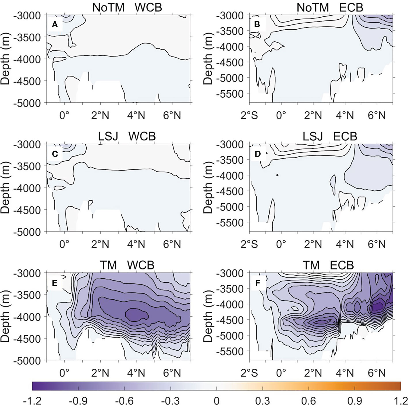
Figure 10 Meridional overturning stream functions (unit: Sv) in the (A, C, E) WCB and (B, D, F) ECB from the experiments (A, B) NoTM, (C, D) LSJ and (E, F) TM, respectively. Negative and positive streamlines correspond to clockwise and counterclockwise circulations, respectively.

4 Summary and discussion

The influence of tidal mixing processes on the bottom water and circulation in the Caroline Sea is investigated in this study by a high-resolution regional model. Three numerical experiments are performed by applying different configurations of diapycnal diffusivity, which are completely without tidal mixing, only with mixing due to local tidal dissipation, and with tidal mixing induced by total (both local and remote) tidal dissipation, respectively. Our results reveal that tidal mixing processes are essential for sustaining a continuous density gradient and thus a persistent baroclinic pressure gradient across the deep-water passages (the YT and EFC) connecting to the open ocean, so as to maintain the large amounts of bottom water transport into the abyssal basins. Moreover, tidal mixing processes can also strengthen the bottom horizontal density gradient within the basins, and thus intensify the bottom basin/subbasin-scale horizontal circulation and MOC. Furthermore, the experiment with tidal mixing shows a more consistent simulation of bottom water transport with previous studies. We found that under the effect of tidal mixing, the LCDW transported into the bottom layer and expected to upwell inevitably to the upper deep layer in the Caroline Sea was about 1.84 Sv, which was very close to previous estimations based on observations. To our knowledge, it is the first time for the observations to be reconstructed by the numerical model. In contrast, the bottom water properties and circulation in both the WCB and the ECB are hardly influenced solely by the local tidal mixing. These results of this study would be useful for further understanding the bottom dynamic processes in the tropical Pacific basins and the detailed components of the global MOC, and could also provide some scientific evidences or references for improving the ocean models by the vertical mixing schemes.

Several uncertainties remain in the present study. First, the local dissipation efficiency (q) was assumed a uniform value of 0.3 in the LSJ02 scheme, while several studies have showed that q is probably heterogeneous in space (St Laurent and Nash, 2004; Falahat et al., 2014; Lefauve et al., 2015). The values of q in the ECB and WCB are in the range 0.1-0.8 estimated by Vic et al. (2019). Thus, the accurate distributions of locally dissipated energy of internal tides remain open to question. Second, the ocean state has a modest but robust and significant sensitivity to the vertical profile of tidal mixing (Melet et al., 2013). However, the current understanding on the spatial distribution of tidal mixing process, especially the vertical distribution of the remote dissipation, remains rather immaturity. Recent theoretical studies (Hibiya et al., 2017; Hibiya, 2022) have shown that, as the tidal advection parameter κUω increases (U is the amplitude of tidal flow; ω is the frequency of tidal flow; κ is the dominant horizontal wavenumber of the seafloor topography), the internal lee waves are generated over seafloor topography and then the vertical decay scale ζ becomes much larger than 500 m. Thus, there is some uncertainty in the vertical structure assumed in the two methods. Moreover, the diapycnal diffusivity of tidal mixing applied in our model is constant in time, which is a simplified statement of reality. It is necessary to embed a tidal mixing scheme into ocean circulation models, in which the completed tidal dissipation process is considered and the calculated diapycnal diffusivities are able to evolve both spatially and temporally with the model state. In addition, turbulent mixing, water properties and circulation structures over the abyssal WCB and ECB remain largely unknown. Therefore, more observations are needed to validate the tidal mixing estimation and improve the simulations in this study.

Under the effect of tidal mixing, the modified LCDW of about 2 Sv in the WCB and ECB could upwell to the upper deep layer of the Caroline Sea (Kawabe and Fujio, 2010). How this modified bottom water would distribute in the upper deep layer of the Pacific Ocean, and whether it could be further modified and continue to upwell somewhere into the intermediate and even the surface layers, are important for the global MOC and the accompanied heat redistribution and materials transport (Kawasaki et al., 2022). These are still open issues and worth investigating in future.

Data availability statement

The raw data supporting the conclusions of this article will be made available by the authors, without undue reservation.

Author contributions

XW: Writing – original draft, Writing – review & editing. CL: Writing – original draft, Writing – review & editing. FW: Writing – original draft, Writing – review & editing.

Funding

The author(s) declare financial support was received for the research, authorship, and/or publication of this article. This work was supported by the National Natural Science Foundation of China (grant number 41806015, 42090044), and the Strategic Priority Research Program of the Chinese Academy of Sciences (grant numbers XDB42040102, XDA22050203).

Conflict of interest

The authors declare that the research was conducted in the absence of any commercial or financial relationships that could be construed as a potential conflict of interest.

Publisher’s note

All claims expressed in this article are solely those of the authors and do not necessarily represent those of their affiliated organizations, or those of the publisher, the editors and the reviewers. Any product that may be evaluated in this article, or claim that may be made by its manufacturer, is not guaranteed or endorsed by the publisher.

References

Atlas R., Hoffman R. N., Ardizzone J., Leidner S. M., Jusem J. C., Smith D. K., et al. (2011). A cross-calibrated, multiplatform ocean surface wind velocity product for meteorological and oceanographic applications. Bull. Amer. Meteor. Soc 92, 157–174. doi: 10.1175/2010BAMS2946.1
Buijsman M. C., Arbic B. K., Richman J. G., Shriver J. F., Wallcraft A. J., Zamudio L. (2017). Semidiurnal internal tide incoherence in the equatorial Pacific. J. Geophys. Res. Oceans 122, 5286–5305. doi: 10.1002/2016JC012590
Egbert G. D., Ray R. D. (2000). Significant dissipation of tidal energy in the deep ocean inferred from satellite altimeter data. Nature 405, 775–778. doi: 10.1038/35015531
Falahat S., Nycander J., Roquet F., Thurnherr A. M., Hibiya T. (2014). Comparison of calculated energy flux of internal tides with microstructure measurements. Tellus A 66, 23240. doi: 10.3402/tellusa.v66.23240
Gent P. R., McWilliams J. C. (1990). Isopycnal mixing in ocean circulation models. J. Phys. Oceanogr. 20, 150–155. doi: 10.1175/1520-0485(1990)020<0150:IMIOCM>2.0.CO;2
Gent P. R., Willebrand J., McDougall T. J., McWilliams J. C. (1995). Parameterizing eddy-induced tracer transports in ocean circulation models. J. Phys. Oceanogr. 25, 463–474. doi: 10.1175/1520-0485(1995)025<0463:PEITTI>2.0.CO;2
Germineaud C., Cravatte S., Sprintall J., Alberty M. S., Grenier M., Ganachaud A. (2021). Deep pacific circulation: New insights on pathways through the Solomon Sea. Deep-Sea Res. I 171, 103510. doi: 10.1016/j.dsr.2021.103510
Hibiya T. (2022). A new parameterization of turbulent mixing enhanced over rough seafloor topography. Geophys. Res. Lett. 49, e2021GL096067. doi: 10.1029/2021GL096067
Hibiya T., Ijichi T., Robertson R. (2017). The impacts of ocean bottom roughness and tidal flow amplitude on abyssal mixing. J. Geophys. Res. 122, 5645–5651. doi: 10.1002/2016JC012564
Jayne S. R., St. Laurent L. C. (2001). Parameterizing tidal dissipation over rough topography. Geophys. Res. Lett. 28 (5), 811–814. doi: 10.1029/2000GL012044
Kaneko I., Takatsuki Y., Kamiya H., Kawae S. (1998). Water property and current distributions along WHP-P9 section (137°–142°E) in the western North Pacific. J. Geophys. Res. 103 (C6), 12959–12984. doi: 10.1029/97JC03761
Kawabe M., Fujio S. (2010). Pacific ocean circulation based on observation. J. Oceanogr. 66, 389–403. doi: 10.1007/s10872-010-0034-8
Kawabe M., Fujio S., Yanagimoto D. (2003). Deep-water circulation at low latitudes in the western North Pacific. Deep-Sea Res. I 50, 631–656. doi: 10.1016/S0967-0637(03)00040-2
Kawasaki T., Matsumura Y., Hasumi H. (2022). Deep water pathways in the North Pacific Ocean revealed by Lagrangian particle tracking. Sci. Rep. 12, 6238. doi: 10.1038/s41598-022-10080-8
Large W. G., McWilliams J. C., Doney S. C. (1994). Oceanic vertical mixing: A review and a model with a nonlocal boundary layer parameterization. Rev. Geophys. 32 (4), 363–403. doi: 10.1029/94RG01872
Lefauve A., Muller C., Melet A. (2015). A three-dimensional map of tidal dissipation over abyssal hills. J. Geophys. Res. Oceans 120, 4760–4777. doi: 10.1002/2014JC010598
Liu X., Liu Y., Cao W., Li D. (2022). Flow pathways of abyssal water in the yap trench and adjacent channels and basins. Front. Mar. Sci. 9, 910941. doi: 10.3389/fmars.2022.910941
Liu X., Liu Y., Cao W., Sun C. (2020). Water characteristics of abyssal and hadal zones in the southern yap trench observed with the submersible Jiaolong. J. Oceanol. Limnol. 38, 593–605. doi: 10.1007/s00343-019-8368-6
Liu Y., Liu X., Lv X., Cao W., Sun C., Lu J., et al. (2018). Watermass properties and deep currents in the Northern Yap Trench observed by the submersible Jiaolong system. Deep Sea Res. Part I 139, 27–42. doi: 10.1016/j.dsr.2018.06.001
Locarnini R. A., Mishonov A. V., Antonov J. I., Boyer T. P., Garcia H. E., Baranova O. K., et al. (2013). “World ocean atlas 2013, volume 1: temperature,” in NOAA Atlas NESDIS 73. Eds. Levitus R. A., Mishonov A. V. (Silver Spring, M.D.: U.S. Department of Commerce), 40 pp.
Marshall J., Adcroft A., Hill C., Perelman L., Heisey C. (1997). A finite-volume, incompressible Navier Stokes model for studies of the ocean on parallel computers. J. Geophys. Res. 102 (C3), 5753–5766. doi: 10.1029/96JC02775
Marshall J., Speer K. G. (2012). Closure of the meridional overturning circulation through Southern Ocean upwelling. Nat. Geosci. 5, 171–180. doi: 10.1038/ngeo1391
Melet A., Hallberg R. W., Legg S., Polzin K. (2013). Sensitivity of the ocean state to the vertical distribution of internal-tide-driven mixing. J. Phys. Oceanogr. 43, 602–615. doi: 10.1175/JPO-D-12-055.1
Munk W., Wunsch C. (1998). Abyssal recipes II: Energetics of tidal and wind mixing. Deep Sea Res. 45, 1977–2010. doi: 10.1016/S0967-0637(98)00070-3
Niwa Y., Hibiya T. (2001). Numerical study of the spatial distribution of the M2 internal tide in the Pacific Ocean. J. Geophys. Res. 106, 22441–22449. doi: 10.1029/2000JC000770
Niwa Y., Hibiya T. (2011). Estimation of baroclinic tide energy available for deep ocean mixing based on three-dimensional global numerical simulations. J. Oceanogr. 67, 493–502. doi: 10.1007/s10872-011-0052-1
Niwa Y., Hibiya T. (2014). Generation of baroclinic tide energy in a global three-dimensional numerical model with different spatial grid resolutions. Ocean Model. 80, 59–73. doi: 10.1016/j.ocemod.2014.05.003
Osborn T. R. (1980). Estimates of the local rate of vertical diffusion from dissipation measurements. J. Phys. Oceanogr. 10, 83–89. doi: 10.1175/1520-0485(1980)010<0083:EOTLRO>2.0.CO;2
Redi M. H. (1982). Oceanic isopycnal mixing by coordinate rotation. J. Phys. Oceanography 12, 1154–1158. doi: 10.1175/1520-0485(1982)012<1154:OIMBCR>2.0.CO;2
Siedler G., Holfort J., Zenk W., Müller T. J., Csernok T. (2004). Deep-water flow in the mariana and caroline basins. J. Phys. Oceanogr. 34, 566–581. doi: 10.1175/2511.1
Smagorinsky J. (1993). “Large eddy simulation of complex engineering and geophysical flows,” in Evolution of Physical Oceanography. Eds. Galperin B., Orszag S. A. (Cambridge: Cambridge University Press), 3–36.
St Laurent L. C., Nash J. (2004). An examination of the radiative and dissipative properties of deep ocean internal tides. Deep-Sea Res. II 51, 3029–3042. doi: 10.1016/j.dsr2.2004.09.008
St. Laurent L. C., Simmons H. L., Jayne S. R. (2002). Estimating tidally driven mixing in the deep ocean. Geophys. Res. Lett. 29 (23), 2106. doi: 10.1029/2002GL015633
Talley L. D. (2013). Closure of the global overturning circulation through the Indian, Pacific, and Southern Oceans: Schematics and transports. Oceanography 26 (1), 80–97. doi: 10.5670/oceanog.2013.07
Vic C., Naveira Garabato A. C., Green J. A. M., Waterhouse A. F., Zhao Z., Melet A., et al. (2019). Deep-ocean mixing driven by small-scale internal tides. Nat. Commun. 10, 2099. doi: 10.1038/s41467-019-10149-5
Wang X., Peng S., Liu Z., Huang R. X., Qian Y. K., Li Y. (2016). Tidal mixing in the South China sea: an estimate based on the internal tide energetics. J. Phys. Oceanogr. 46, 107–124. doi: 10.1175/JPO-D-15-0082.1
Zhao Z., Alford M. H., Girton J. B., Rainville L., Simmons H. L. (2016). Global observations of open-ocean mode-1 M2 internal tides. J. Phys. Oceanography 46 (6), 1657–1684. doi: 10.1175/JPO-D-15-0105.1
Zhao J., Cheng H., Cao J., Sinha A., Dong X., Pan L., et al. (2023). Orchestrated decline of Asian summer monsoon and Atlantic meridional overturning circulation in global warming period. Innovation Geosci. 1 (1), 100011. doi: 10.59717/j.xinn-geo.2023.100011
Keywords: bottom water, bottom circulation, tidal mixing, Caroline Sea, West Caroline Basin, East Caroline Basin, ocean model
Citation: Wang X, Liu C and Wang F (2024) Influence of tidal mixing on bottom circulation in the Caroline Sea. Front. Mar. Sci. 11:1301541. doi: 10.3389/fmars.2024.1301541
Received: 25 September 2023; Accepted: 18 January 2024;
Published: 13 February 2024.
Edited by:
Toru Miyama, Japan Agency for Marine-Earth Science and Technology, JapanReviewed by:
Gengxin Chen, Chinese Academy of Sciences (CAS), ChinaTakao Kawasaki, The University of Tokyo, Japan
Copyright © 2024 Wang, Liu and Wang. This is an open-access article distributed under the terms of the Creative Commons Attribution License (CC BY). The use, distribution or reproduction in other forums is permitted, provided the original author(s) and the copyright owner(s) are credited and that the original publication in this journal is cited, in accordance with accepted academic practice. No use, distribution or reproduction is permitted which does not comply with these terms.
*Correspondence: Chuanyu Liu, chuanyu.liu@qdio.ac.cn