Rule-based semi-automated tools for mapping seabed morphology from bathymetry data

1 Introduction

Seabed morphology, as often identified and mapped from bathymetry data, describes the geometry of discrete physical features on the seafloor. Seabed morphology maps provide fundamental information for a range of applications, including mapping coastal and marine habitats (e.g., Erdey-Heydorn, 2008; Micallef et al., 2012; Smith et al., 2015), interpreting seabed geomorphology and its formative processes (e.g., Micallef et al., 2018; O’Brien et al., 2020; Nanson et al., 2022), and understanding seabed stability and sediment dynamics (e.g., O’Brien et al., 2015; Picard et al., 2018b; Nanson et al., 2022; Post et al., 2022). The increasing availability of bathymetry data (e.g., AusSeabed, https://www.ausseabed.gov.au/; Wölfl et al., 2019) has supported the application of seabed morphology and geomorphology mapping at a wide-range of spatial scales (e.g., Ferrini and Flood, 2005; Heap and Harris, 2008; Harris et al., 2014; Huang et al., 2014; Linklater et al., 2015; Picard et al., 2018a; O’Brien et al., 2020; Post et al., 2020; Weinstein et al., 2021; Nanson et al., 2022; Post et al., 2022).

With the increased demand for seabed morphology and geomorphology maps to support ocean science, management and policy there is a pressing need for mapping and classification standards to ensure consistency between sub-disciplines and disparate mapping regions (Dove et al., 2020). Heap and Harris (2008) and Harris et al. (2014) mapped the regional- to global-scale distribution of seabed geomorphic features of the Australian margin and the global oceans, respectively, using terminology that was primarily drawn from the International Hydrographic Organization’s standardised list of undersea feature names (IHO, 2001; IHO, 2008). Dove et al. (2016) similarly drew on this internationally-adopted list of terms, and proposed a novel two-part approach whereby morphological mapping (and classification) is applied separately to the geomorphological classification of each feature. Using this two-part approach, Morphological Features can be characterised by their surface expression (i.e., size, shape, configuration, texture: Part 1 - Dove et al., 2020; note their intentional capitalising of these defined terms as proper nouns), whereas their (subsequent) geomorphic interpretation incorporates knowledge of the environmental process(es) by which they formed (Part 2 - Nanson et al., 2023).

Dove et al. (2020) defined 17 bathymetric high and 14 bathymetric low Morphology Features, using qualitative terms primarily sourced from the IHO (IHO, 2019), and provided an illustrated glossary. These bathymetric high (low) Features which are elevated (depressed) relative to the adjacent seafloor are the targets of the semi-automated bathymetric mapping tools described in this paper. Though Dove et al. (2020) provided only a few dimensional and geometric thresholds for categorical bathymetric classification (e.g. Seamounts must exceed 1000 m in depth range; Mounds must be less than 500 m in depth range), they recommended the development of more comprehensive criteria for the practical implementation of their approach (e.g., shape elongation, topographic gradient and profile symmetry). Importantly, Dove et al. (2020) also emphasised that mapped Morphology Features need not share common spatial boundaries; overlapping seabed Features are common (e.g. Mounds on a Plain) and can provide useful insights into relationships between them (e.g., pockmarks and depressions on plains; Picard et al., 2018b). As a result, mapped Features need not be spatially unique and do not need to adhere to rigid topology principles. These attributes of the Dove et al. (2020) approach determine that the mapping of Morphology Features can be approached using a variety of spatial analyst and image processing techniques that we present in this paper.

Manual and semi-automated methods are frequently used to map seabed features. Many seabed morphological features such as canyons, seamounts, ridges, valleys, banks and depressions have distinct geometries. Consequently, visual interpretations and manual digitisation have often been used to define their extents, sometimes with the support of ancillary data (e.g., Beaman and Harris, 2005; Ferrini and Flood, 2005; Heap and Harris, 2008; Nichol and Brooke, 2011; Nichol et al., 2011; Sacchetti et al., 2011; Huang et al., 2014; Linklater et al., 2015; Tecchiato et al., 2015; O’Brien et al., 2020; Post et al., 2022). The manual mapping method has the advantage of being able to implicitly incorporate domain knowledge and contextual information while tolerating data quality issues. However, the manual mapping method also suffers from subjectivity and, importantly, it is not repeatable in delineating feature boundaries. Critically, the manual mapping method can be prohibitively time consuming and impractical for mapping large numbers of small features in complex seabed environments. Semi-automated mapping tools have since been developed to address these issues.

Semi-automated mapping methods can be unsupervised, supervised or rule-based. Both unsupervised (including object-based segmentation) and supervised mapping techniques aim to divide an area of interest into mutually exclusive classes by maximising between-class variation and minimising within-class variation so that each class is “uniform” in properties. Few cases of seabed morphology mapping have applied either the unsupervised (Jones and Brewer, 2012; Ismail et al., 2015) or the supervised (Lanier et al., 2007) methods. This likely reflects the fact that it is challenging to apply these mapping techniques to complex real world seabed morphological features, such as canyons or seamounts, which do not have “uniform” bathymetric properties. In contrast, the rule-based methods explicitly apply domain knowledge and can be designed to classify complex seabed morphological features. Once the rules are determined by domain experts, these methods can be applied objectively, consistently and efficiently in a GIS environment. Consequently, many previous seabed morphology mapping applications have employed the rule-based methods (e.g., Lundblad et al., 2006; Lanier et al., 2007; Erdey-Heydorn, 2008; Zieger et al., 2009; Micallef et al., 2012; Harris et al., 2014; O’Brien et al., 2015; Jerosch et al., 2016; Picard et al., 2018b; Hebbeln et al., 2019; Lavagnino et al., 2020; Sowers et al., 2020; Weinstein et al., 2021).

Classification rules to map seabed morphology can be based on bathymetry data and/or its derivatives such as Topographic Position Index (TPI; Weiss, 2001), fuzzy morphometrics (Fisher et al., 2004) and geomorphons (Jasiewicz and Stepinski, 2013). The TPI technique is able to map six broad morphological classes (Weiss, 2001) and, with the help of additional slope gradient and bathymetry data, 13 detailed morphological classes (Lundblad et al., 2006; Erdey-Heydorn, 2008). The fuzzy morphometric based technique is able to map six morphological classes, and the geomorphon based technique is able to map 10 morphological classes. Each of these three techniques require the setting of appropriate scale parameters (e.g., window size or distance) to map seabed features of various spatial scales. However, none of these out-of-the box tools are able to adequately map the Morphology Features of the Dove et al. (2020) scheme.

In this study we have developed a semi-automated, rule-based mapping method to target the mapping of ten bathymetric high and eight bathymetric low seabed Morphological Features as defined by Dove et al. (2020). This paper aims to describe this new method, which is implemented as a number of GIS tools (Figure 1; Huang et al., 2022). We also evaluated the performance of these tools through their application to a diverse suite of bathymetry datasets as case studies that represent a spectrum of Features that characterise the Australian and Antarctic margins. In addition, we conducted a controlled experiment to provide more quantitative comparisons between manual mapping and our semi-automated mapping at one of the case study areas. Lastly, we discuss the benefits and limitations of these semi-automated tools based on the results of these case studies.

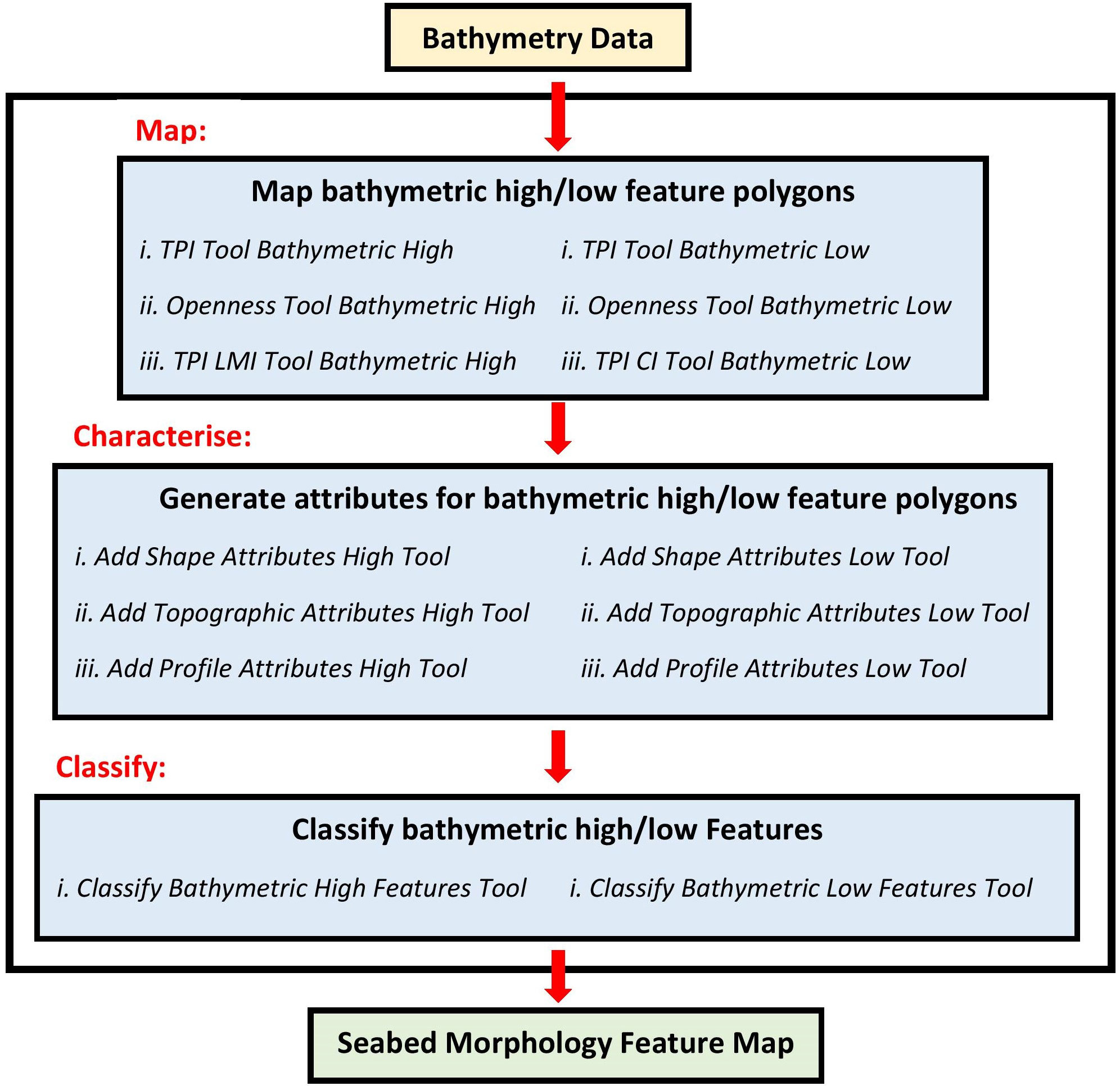
Figure 1 Flow Chart of the semi-automated mapping tools (GA-SaMMT). There are three sequential steps: Map (Step 1), Characterise (Step 2) and Classify (Step 3). TPI stands for Topographic Position Index; LMI stands for Local Moran’s Index; CI stands for Convergence Index.

2 Materials and methodology

2.1 Overview of the semi-automated mapping method

The semi-automated seabed morphology mapping method (Geoscience Australia’s Semi-automated Morphological Mapping Tools (GA-SaMMT)) implements a three-step solution – Map, Characterise and Classify (Figure 1). The Map step (Step 1) delineates polygons that outline High and Low features; The Characterise step (Step 2) generates attributes (metrics) to describe the geometry of the mapped polygons from the Map Step; while, the Classify step (Step 3) uses the attributes generated from the Characterise step to assign a Morphology Feature type to each mapped polygon (Figure 1). For each of these three steps a number of ESRI ArcGIS Pro Python tools with graphical user interfaces have been developed to streamline their implementation (Huang et al., 2022; https://dx.doi.org/10.26186/146832).

The subjective components of the semi-automated mapping method are: 1) the requirement for several user inputs as tool parameters; and 2) potential requirement of manual post editing/modification of feature polygon shapes and their classification to obtain an optimal product. These user inputs are necessary to maintain flexibility in mapping Morphology Features at a range of spatial scales and with application-specific conditions. Fundamentally, these user inputs are also required to utilise the additional local domain knowledge of the analyst. Manual editing post GA-SaMMT - Map step may also be needed in some applications to fine-tune the feature boundary and to fix unsatisfactory mapping results of some individual features that are inherited from underlying data quality issues and the inherent complexity of these features.

GA-SaMMT possesses the same advantages of other rule-based mapping methods, including the ability to use domain knowledge, repeatability, boundary accuracy and time-efficiency. Importantly, this semi-automated method operationalises the Dove et al. (2020) seabed morphology classification scheme that offers consistency between study areas. Another key advantage of this semi-automated method is its ability and flexibility to map Morphology Features at a wide-range of spatial scales on a single dataset, from very-fine scale Features such as Hummocks and small Holes/Depressions to broad scale Features such as Seamounts and Canyons. In addition, this semi-automated method offers flexibility for continuous future development, for example to include more mapping tools and to modify the publicly accessible scripts for advanced users. GA-SaMMT are described below in detail.

2.1.1 Mapping bathymetric high/low feature polygons (GA-SaMMT Map; Step 1)

The objective of this first step is to identify and map the polygon boundaries of individual bathymetric high and low features from the input bathymetry data. We developed three ArcGIS Pro Python tools to map bathymetric high and low Features separately (Figures 1, S1-S3). These tools target the mapping of ten bathymetric high Features and eight bathymetric low Features, following the definitions in Dove et al. (2020) (Table 1; Figure 2). These 18 Feature types are a subset of the 31 Morphology Features defined by Dove et al. (2020) that are selected here because they represent commonly targeted morphologies for applications such as habitat mapping, and they have the best potential for capture by semi-automated mapping. Specifically, they have higher (or lower) elevations than the surrounding bathymetric surface. Most of the remaining 13 Feature types defined in Dove et al. (2020) (those greyed out in Figure 2), such as Terrace, Apron, Peak, Floor, Saddle and Gap, require additional steps after mapping the 18 principal bathymetric high and low Features. In addition, a few of the 13 Features such as Block and Fan are also more difficult to map by semi-automation due to their complex definitions (Dove et al., 2020). We will attempt to develop semi-automated tools to map these 13 remaining bathymetric high and low Feature types in future versions of GA-SaMMT. Note that Dove et al. (2020) refer to these Feature types as proper nouns, such that reference to these Features and more specific Feature types (e.g., Seamount, Canyon) are capitalised. Where we refer to mapping by earlier workers who used other classification schemes (i.e. not Dove et al., 2020), their terms remain uncapitalised (e.g., channels, ridges).

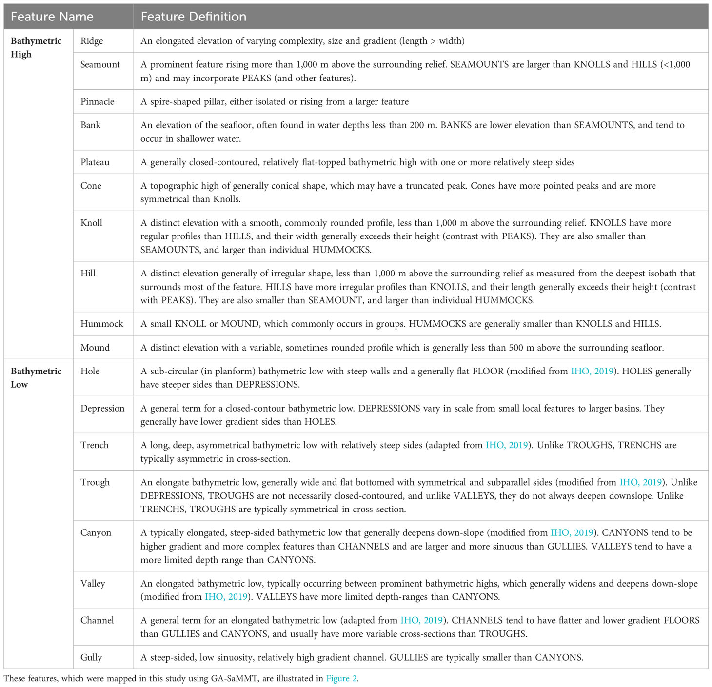
Table 1 Definitions of 18 bathymetric high and low features according to Dove et al. (2020).

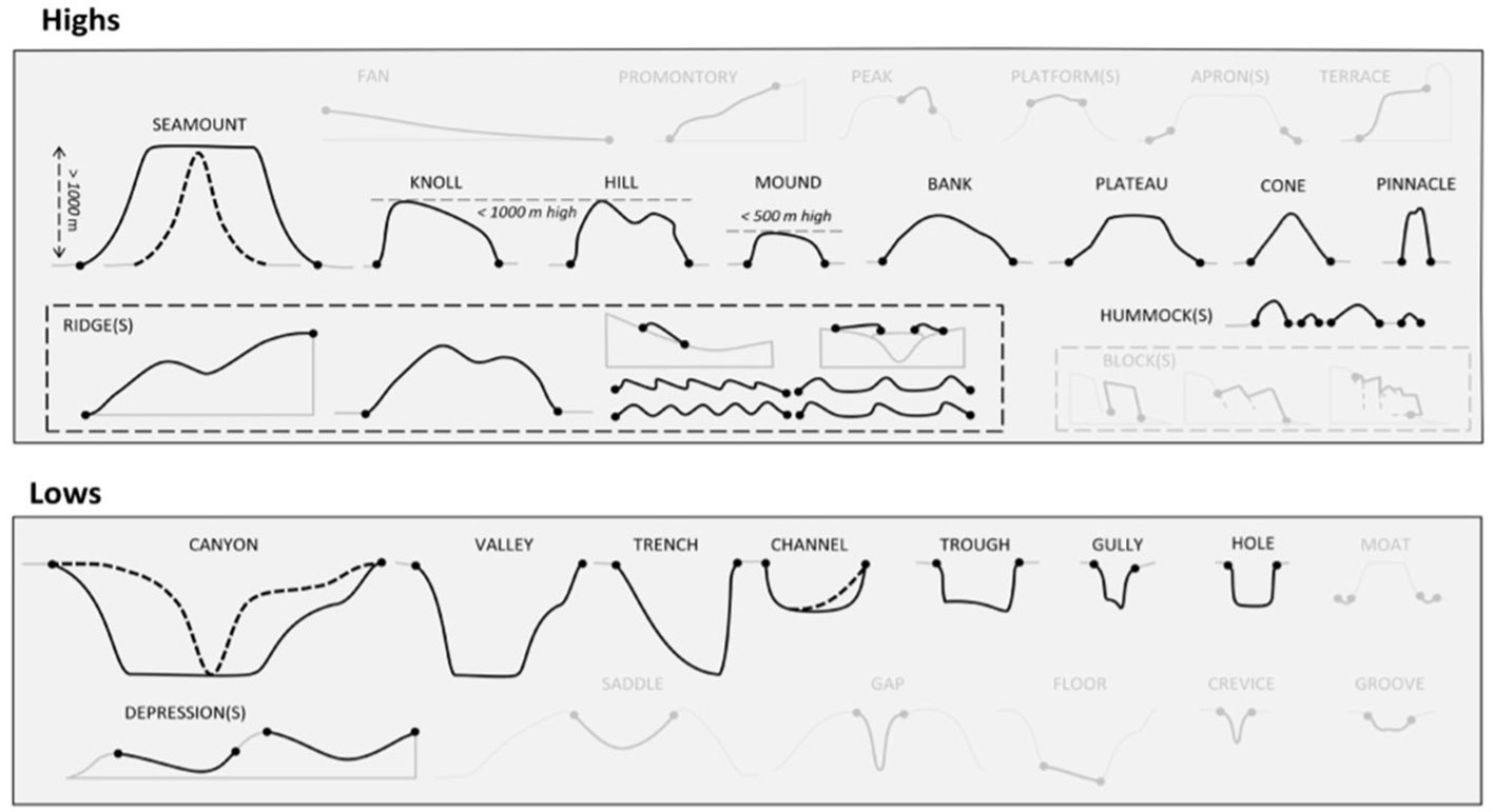
Figure 2 The idealised cross-section profiles of the bathymetric high and low Features modified from Dove et al. (2020). The greyed out Features are not implemented by the current version of GA-SaMMT.

2.1.1.1 TPI tools

The Topographic Position Index (TPI) method, which compares the elevation of the centre cell to the mean elevation of a specified neighbourhood around the cell (Weiss, 2001), has been used extensively to map seabed morphological classes (e.g., Lundblad et al., 2006; Erdey-Heydorn, 2008). This is mainly because a positive (or negative) TPI value (in metres) indicates a bathymetric high (or low) location. Our ‘TPI Tool Bathymetric High’ and the ‘TPI Tool Bathymetric Low’ ArcGIS Pro Python tools (Figure S1) similarly implements the TPI (Weiss, 2001) method to map bathymetric high and low feature polygons from bathymetric data using the following steps:

1. Calculate TPI raster from the input bathymetry raster using the following equation:

where x and y are the positions of the centre cell, E_x,y is the elevation (bathymetry) value at the centre cell and WD_x,y is the mean elevation (bathymetry) within a neighbourhood window defined by the “TPI Circle Radius” parameter, which is calculated using the ArcGIS Focal Statistics function.

2. Calculate the TPI threshold using Equation 2 for bathymetric high Features or Equation 3 for bathymetric low Features

where TPI_T is the TPI threshold, TPI_m and TPI_s are the spatial mean which represents the “neutral” condition and the standard deviation statistics of the TPI raster, respectively, and C_TPI is the “TPI STD Scale” parameter.

3. Select locations that have TPI values greater (or lower) than the TPI threshold.

4. Convert the selected areas into polygons.

5. Remove the feature polygons with areas smaller than the “Area Threshold” parameter to obtain the final set of bathymetric high (or low) feature polygons as output.

Note that these three parameters (“TPI Circle Radius”, “TPI STD Scale” and “Area Threshold”) have influence on the mapping results. Users need to experiment with different combinations of these parameters to obtain an optimal mapping result with the guidance of a domain expert. For the “TPI Circle Radius” parameter, a rule of thumb is to use a radius slightly larger than the largest bathymetric high (or low) Features to be mapped in the area of interest. For example, for a 5 m resolution bathymetry raster, a radius of 50 cells should be used to capture any bathymetric high Features that are smaller than 500 m in length. This is also the case for other mapping tools outlined below (Openness, TPI LMI and TPI CI in Figure 1). In addition, to capture multiple scales of seabed Morphology Features (e.g., Seamounts, Mounds and Hummocks) in a single bathymetry dataset, several separate applications of the TPI tool using various TPI radius parameters are often required.

For the “TPI STD Scale” parameter (and the similar parameters in other mapping tools described in sections 2.1.1.2 and 2.1.1.3), the diversity and complexity of individual applications means that it is not possible to provide a rule of thumb for the parameter value. Instead, users need to experiment to find the most appropriate parameter values for their dataset.

Users should also adjust C_TPI, which is a multiplicative factor, so that the TPI_T has a positive (or negative) value for bathymetric high (or low) features. The same is required for similar parameters for the other mapping tools that follow.

2.1.1.2 Openness tools

The ‘Openness Tool Bathymetric High’ and the ‘Openness Tool Bathymetric Low’ ArcGIS Pro Python tools (Figure S2) are used to map bathymetric high (low) feature polygons from bathymetric data using an openness based method (Yokoyama et al., 2002). Openness indicates the degree of dominance or enclosure of a location on a surface by calculating an angular measure of the relation between surface relief and horizontal distance (Yokoyama et al., 2002). The openness can be calculated as negative openness (NO) which represents the “below-ground” view of the landscape and positive openness (PO) which represents the “above-ground” view of the landscape. Both NO and PO range from 0 to 180 degree. Either NO or PO can be used to identify both bathymetric high (convex) and bathymetric low (concave) locations (Yokoyama et al., 2002). In this study, we used NO (or PO) to map bathymetric high (or low) Features because a NO (or PO) value that is smaller than the mean (i.e., the “neutral” condition) indicates a bathymetric high (or low) location. Again, these two Openness tools implement similar steps as follows:

1. Calculate NO (or PO) from the input bathymetry raster using the “Openness Circle Radius” parameter.

2. Identify the possible ‘tops’ (or ‘bottoms’) of the bathymetric high (or low) Features from the inversed (or normal) bathymetry raster based on the ArcGIS Sink function which is able to find cell(s) that are lower than all neighbouring cells (Mark, 1988).

3. For the bathymetric high Features, calculate the NO threshold using Equation 4.

where NO_T is the NO threshold, NO_m and NO_s are the spatial mean (i.e., the “neutral” condition) and standard deviation statistics, respectively, of the NO raster, and C_NO is the “NO STD Scale Large” parameter or the “NO STD Scale Small” parameter. For the bathymetric low Features, calculate the PO threshold using Equation 5.

where PO_T is the PO threshold, PO_m and PO_s are the spatial mean (i.e., the “neutral” condition) and standard deviation statistics of the PO raster, and C_PO is the “PO STD Scale Large” parameter or the “PO STD Scale Small” parameter.

4. Select the first set of areas that have NO (or PO) values smaller than the “NO STD Scale Large” (or “PO STD Scale Large”) threshold.

5. Select the second set of areas that have NO (or PO) values smaller than the “NO STD Scale Small” (or “PO STD Scale Small”) threshold.

6. Further select from the two sets of areas only those areas that contain ‘tops’ (or ‘bottoms’).

7. These two new sets of areas are used together to identify individual bathymetric high (or low) Features, through GIS overlay and selection functions.

8. If any polygons in the second set contain more than one polygons in the first set, the multiple polygons from the first set are selected as the first subset.

9. If any polygons in the second set contain only one polygon in the first set, the polygons from the second set are selected as the second subset.

10. Merge the above two subsets of polygons together to form a set of bathymetric high (or low) feature polygons

11. Remove the feature polygons with areas smaller than the “Area Threshold” parameter to obtain the final set of bathymetric high (or low) feature polygons as output.

2.1.1.3 TPI LMI and TPI CI tools

The ‘TPI LMI Tool Bathymetric High’ ArcGIS Pro Python tool (Figure S3A) maps bathymetric high feature polygons using a combination of TPI (Weiss, 2001) and Local Moran’s Index (LMI) (Moran, 1950; Anselin, 1995) methods. Positive TPI indicates a bathymetric high location. LMI measures spatial autocorrelation based on both locations and values within a nominated local area. As a result, positive LMI indicates a spatial pattern of positive (higher than average) local auto-correlation (in this case a similar local pattern of (or clustered) higher bathymetry values). The following are the key steps of this tool:

1. Calculate TPI from the input bathymetry raster using the “TPI Circle Radius” parameter using Equation 1.

2. Calculate the TPI thresholds using Equation 2, only this time C_TPI is the “TPI STD Scale Large” parameter or the “TPI STD Scale Small” parameter. Note that the TPI thresholds should always have positive values.

3. Select the first set of areas that have TPI values greater than the “TPI STD Scale Large” threshold.

4. Select the second set of areas that have TPI values greater than the “TPI STD Scale Small” threshold.

5. These two sets of areas and the bathymetry data are used together to select the ‘core’ areas of bathymetric high Features, through GIS overlay and selection functions.

6. These ‘core’ areas are masked from the bathymetry data.

7. Calculate LMI from the masked bathymetry raster using the “LMI Weight File” parameter, which is an ASCII text file that defines the shape of the neighbourhood and the weight of each cell in that neighbourhood.

8. Calculate the LMI thresholds using Equation 6.

Where LMI_T is the LMI threshold, LMI_m and LMI_s are the spatial mean and standard deviation statistics of the LMI raster, respectively, C_LMI is the “LMI STD Scale” parameter. Note that the LMI threshold should always have a positive value.

9. Select locations from the LMI raster that have LMI values greater than the LMI threshold. These locations (areas) are regarded as the remaining parts of bathymetric high Features.

10. Merge the ‘core’ areas and the ‘remaining’ parts of bathymetric high Features to form individual bathymetric high Features.

11. Remove the feature polygons with areas smaller than the “Area Threshold” parameter to obtain the final set of bathymetric high feature polygons.

Similar user advice and the rule of thumb for the “TPI Circle Radius” parameter are applicable.

The ‘TPI CI Tool Bathymetric Low’ ArcGIS Pro Python tool (Figure S3B) maps bathymetric low feature polygons from bathymetric data using a combination of TPI (Weiss, 2001) and Convergence Index (CI) (Koethe and Lehmeier, 1996; Kiss, 2004; Thommeret et al., 2010) methods. Negative TPI indicates a bathymetric low location. The CI, which is based on the aspect (i.e., slope direction), indicates areas of convergence and divergence (Koethe and Lehmeier, 1996; Kiss, 2004; Thommeret et al., 2010); negative CI also indicates a location of convergence (or bathymetric low). The following are the key steps of this tool:

1. Calculate the Aspect raster from the input bathymetry raster.

2. Calculate CI from the Aspect raster using the following equation (Koethe and Lehmeier, 1996; Kiss, 2004; Thommeret et al., 2010):

Where θ_i is the angle in degrees between the aspect of cell i and its direction to the centre cell of a 3×3 neighbourhood window.

3. Calculate TPI from the input bathymetry raster using the “TPI Circle Radius” parameter.

4. Calculate the CI threshold (CI_T) using Equation 8.

Where CI_m and CI_s are the spatial mean and standard deviation statistics of the CI raster, respectively, and C_CI is the “CI STD Scale” parameter. The CI threshold should always have a negative value.

5. Calculate the TPI threshold using Equation 3. The TPI threshold should always have a negative value.

6. Select the first set of areas that have CI values smaller than the CI threshold.

7. Select the second set of areas that have TPI values smaller than the TPI threshold.

8. Merge the two sets of areas together to form a set of bathymetric low feature polygons.

9. Remove the feature polygons with areas smaller than the “Area Threshold” parameter to obtain the final set of bathymetric low feature polygons as output.

2.1.2 Characterising bathymetric high/low feature polygons (GA-SaMMT Characterise; Step 2)

After the polygon boundary of each bathymetric high/low feature has been mapped a range of attributes are calculated to characterise the geometry of each feature polygon (Figure 1). Subsets of these feature attributes are subsequently used to classify each feature polygon into a Morphology Feature type (Step 3: detailed in section 2.1.3).

We developed three ArcGIS Pro Python tools to calculate the shape, topographic and profile attributes of bathymetric high and low feature polygons in a sequential order (Figures 1, S4–S6). The shape attributes are metrics calculated from the horizontal (planform) shape of each mapped feature polygon and the vertical (cross-sectional) dimensions of the feature (Figure 3A; Table 2). The topographic attributes are metrics calculated from the bathymetry and slope gradient data (Figure 3B; Table 3). The profile attributes are metrics derived from selected cross-section profile(s) (Figure 3C; Table 4). As a result, these three classes of attributes represent different and diverse characteristics of a mapped feature.

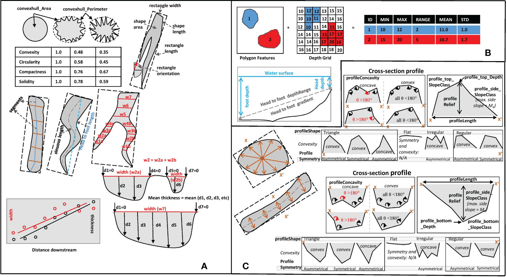
Figure 3 Graphic illustrations of the shape attributes (A), topographic attributes (B) and profile attributes (C) listed in Tables S1–S3.

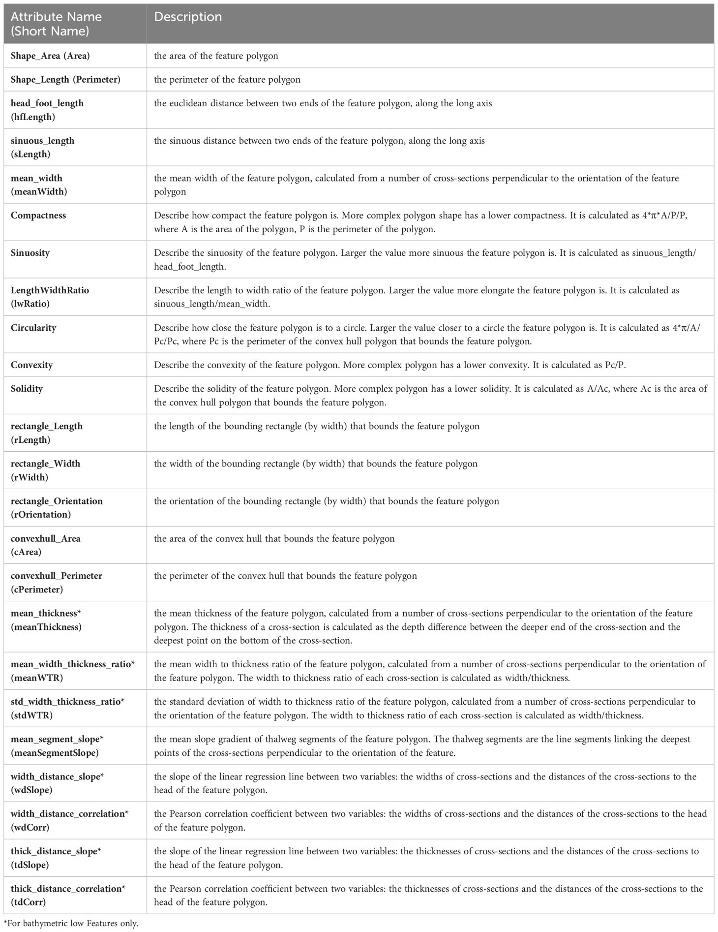
Table 2 Shape attributes for bathymetric high and low features (these attributes are illustrated in Figure 3A).

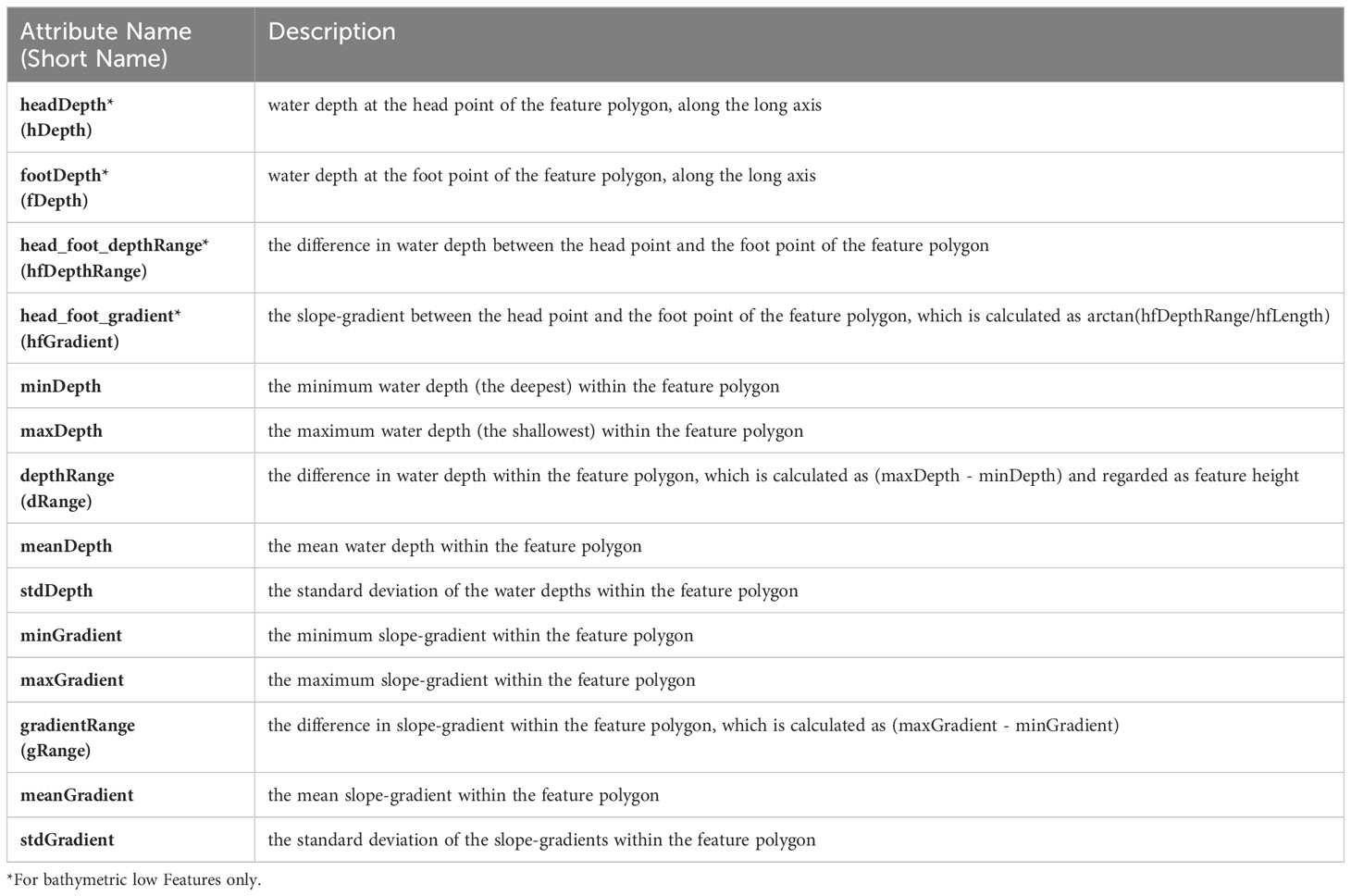
Table 3 Topographic Attributes for bathymetric high and low features (these attributes are illustrated in Figure 3B).

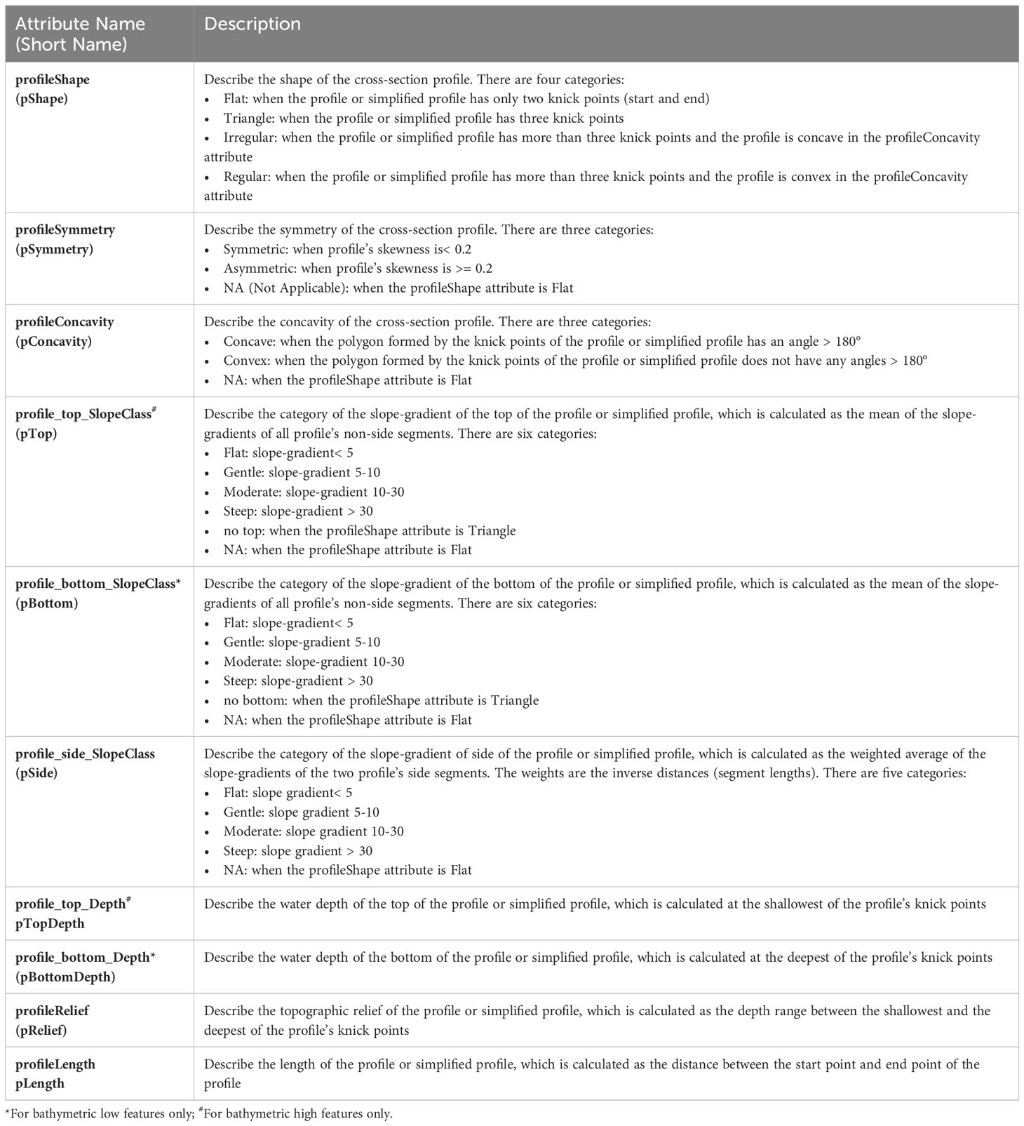
Table 4 Profile attributes for bathymetric high and low features (these attributes are illustrated in Figure 3C).

Importantly, these “characterise” tools can also be applied to feature polygons mapped using manual or other semi-automated methods. The ‘Add Shape Attributes High Tool’ and the ‘Add Shape Attributes Low Tool’ ArcGIS Pro Python tools (Figure S4) calculate 16 and 24 shape attributes for bathymetric high and bathymetric low feature polygons, respectively (Table 2; Figure 3A). The ‘Add Topographic Attributes High Tool’ and the ‘Add Topographic Attributes Low Tool’ ArcGIS Pro Python tools (Figure S5) calculate 10 and 14 topographic attributes for bathymetric high and bathymetric low feature polygons, respectively (Table 3; Figure 3B).

For each bathymetric high (or low) feature polygon, if its area is smaller than a user-defined threshold, the ‘Add Profile Attributes High Tool’ (or the ‘Add Profile Attributes Low Tool’) ArcGIS Pro Python tool (Figure S6) generates one cross-section profile passing through the polygon centre. If, however, the feature area is larger than a user-defined threshold and the polygon is not elongated, then the tool generates five cross-section profiles passing through the polygon centre, with an equal-angle interval. Otherwise, the tool generates five cross-section profiles perpendicular to the orientation of the feature polygon, with an equal-distance interval (Figure 3C). A cross-section profile is formed by the bathymetry values at a series of points along the profile. The number of points in this profile is determined by the length of the profile. This profile is then simplified if we can identify and link a subset of original points as breaks-in-slope points across the profile. Note that a break-in-slope point is a knickpoint that is determined by identifying a sharp change in slope. Also note that, in this case, the start and end points of a cross-section profile are always retained as breaks-in-slope points. After that, eight attributes, which are illustrated in Figure 3C, are calculated to characterise the cross-section profile(s) [or simplified profile(s)] (Table 4).

2.1.3 Classifying bathymetric high/low features (GA-SaMMT Classify; Step 3)

After attributes have been calculated for each bathymetric high (or low) feature polygon, the last semi-automated step is to classify each feature polygon into one of the 18 high and low Feature types (Figure 1). The two ArcGIS Pro Python tools developed for this step are shown in Figure S7.

2.1.3.1 Classification rules for bathymetric high Features

We developed a set of rules for the classification of bathymetric high Features (Figures 4A, S8A) and the classification of bathymetric low Features (Figures 4B, S8B). These rules were modified from the classification scheme of Dove et al. (2020) for their individual Feature types (Table 1; Figure 2). For those few Feature definitions for which they defined quantitative threshold values (e.g., Seamount and Mound; Table 1; Figure 2), these values are hardcoded within the classification rules (Figures 4A, S8A). For most other features with only qualitative definitions, the threshold values are implemented as user-defined tool parameters with suggested default threshold values (Figures 4, S7, S8). This provides flexibility for users to choose appropriate threshold values to suit specific applications. This flexibility also allows users to experiment with these threshold values and apply this step iteratively to achieve optimal classification results.

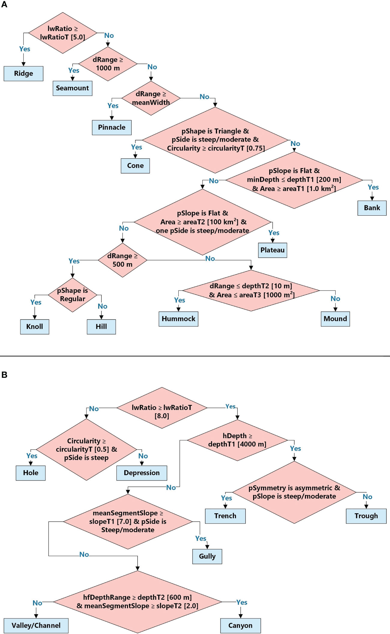
Figure 4 Classification rules illustrated as tree diagrams; (A) bathymetric high Features; (B) bathymetric low Features; Notes (lwRatioT: LengthWidthRatio Threshold, areaT1: area threshold 1, areaT2: area threshold 2, areaT3: area threshold 3, depthT1: depth threshold 1, depthT2: depth threshold 2, slopeT1: slope threshold T1, slopeT2: slope threshold T2, circularityT: circularity threshold); attribute short names are listed in Tables 2–4. The values within the square brackets [] are suggested default threshold values.

The classification rules for the bathymetric high Features (Figures 4A, S8A) separate Ridges from other Features using a threshold for their elongation attribute [measured by the lwRatio attribute (Table 2)], as defined by Dove et al. (2020) (Table 1). Feature height [measured by the dRange attribute (Table 3)] is subsequently used to separate three groups of bathymetric high Features: Seamounts (≥ 1000 m), Knolls/Hills (500 – 999 m) and Mounds/Hummocks (< 500 m). This follows the definitions and the cross-section profiles presented in Dove et al. (2020) (Table 1; Figure 2). Knolls and Hills are distinguished by calculating the regularity of their profiles [measured by the pShape attribute (Table 4)] (Table 1). Hummocks are distinguished from smaller Mounds by assigning them smaller areas [measured by the Area attribute (Table 2)] and feature heights (Figure 4A). The definition of Pinnacles as spire-shaped pillars (Table 1) is incorporated into a rule specifying that its feature height must be larger than its width [measured by the meanWidth attribute (Table 2)] (Figures 4A, S8A). As Cones have conical and symmetrical profiles (Table 1) the relevant rule captures those with circular polygons [measured by the Circularity attribute (Table 2)] with triangular and moderate to steep side-profiles [measured by the pSide attribute (Table 4)] (Figures 4A, S8A).

The classification rules for Banks and Plateaus are slightly more complicated because their definitions are not distinctly different from other Feature types such as Mounds, Knolls and Hills (Dove et al., 2020). Considering Plateaus are defined as flat-topped features and Banks are also often considered as flat-topped compared to Mounds, Knolls and Hills, we specified a rule condition that Plateaus and Banks must be flat (measured by the compound attribute of pSlope) (Figures 4A, S8A). The pSlope attribute is calculated as the pTop attribute (Table 4) when pTop ≠ ‘no top’ and as the pSide attribute (Table 4) when pTop = ‘no top’. In addition, because Plateau is defined as having one or more relatively steep sides (Table 1), one condition was added to specify that the slope of at least one of its profile(s) is moderate or steep (Figures 4A, S8A). Moreover, because IHO (2019) defines Plateaus as large features, we added an additional area condition (Area ≥ 100 km²) to its classification rule (Figures 4A, S8A). Bank is often considered as a relatively large feature, we thus also added an area condition (Area ≥ 1.0 km²) to its classification rule (Figures 4A, S8A). In addition, Bank is defined as occurring in shallower water (≤ 200 m) [measured by the minDepth attribute (Table 3)] (Table 1) which is reflected in the corresponding classification rule (Figures 4A, S8A).

2.1.3.2 Classification rules for the bathymetric low Features

The classification rules for the bathymetric low Features (Figures 4B, S8B) separate Hole and Depression from other Features based on the elongation attribute, according to the Feature definitions presented in Table 1. Between Hole and Depression, the separation is based on the circularity of the polygon shape and the gradient of the profile side [measured as the pSide attribute (Table 4)] as defined (Table 1). Note that the important criterion of ‘a closed-contour bathymetric low’ in the definition of Depression (Table 1) creates a mapping challenge (as follows), and was unable to be implemented in the current version of GA-SaMMT. Though the contour function in GIS software such as ArcGIS and QGIS can generate contour (poly-)lines that capture many of the bounding vertices of a Depression, these polylines may not join at their end points to form closed contour polygons [e.g. the polyline encircling the Depression simply may not close between the final two vertices; the contour may continue beyond the Depression where a bedform (high) intersects the boundary of a scour (low)]. In addition, the selection of an appropriate contour interval is problematic because many thousands of tiny depressions (e.g. pockmarks) may be represented by only a small number of cells [e.g., in the case study of Bonaparte Basin (section 3.3 below)]. None of the current set of attributes listed in Tables 2–4, which are based on topography, the horizontal and vertical shapes of the feature polygon, are able to provide suitable proxies to measure closed-contour criterion. New attribute(s) are needed for this purpose and are the focus of future work.

For the remaining elongated features, we used water depth of the feature head [measured as the hDepth attribute (Table 3)] to separate Trench and Trough from Canyon, Gully, Valley, and Channel. Essentially, we considered Trench and Trough as features occurring in deep water. This is because Trench is defined as a deep feature (Table 1); while Trough is often considered as being located in a similar water depth setting as Trench. In addition, Harris and Whiteway (2011) defined that a canyon head must be located in a water depth shallower than 4,000 m. This provides us a reasonable depth value (depthT1 in Figures 4B, S8B) of 4,000 m as the default threshold to separate Trench/Trough from other elongated bathymetric low Features. Between Trench and Trough, Trench is asymmetrical in cross-section [measured by the pSymmetry attribute (Table 4)] and has a steeper bottom (measured by the compound attribute of pSlope) than Trough (Table 1). This is reflected in the corresponding classification rule for these two Features (Figures 4B, S8B). The pSlope attribute, in this case, is calculated as the pBottom attribute (Table 4) when pBottom ≠ ‘no bottom’ and as the pSide attribute when pBottom = ‘no bottom’.

Among the other classes of elongated bathymetry low Features (Gully, Canyon, Valley and Channel), Gully is defined as steep-side and relatively high-gradient channel (Table 1), so the pSide attribute (Table 4) and the meanSegmentSlope attribute (Table 2) are used to capture these two characteristics, respectively. Canyons tend to have larger head-to-foot depth ranges than Valleys and higher gradients than Channels (Table 1; Huang et al., 2014). Therefore, the hfDepthRange attribute (Table 2) and the meanSegmentSlope attribute are used in the classification rule to separate Canyon from Valley and Channel (Figure 4B). The geometry of Gibling (2006), and the definitions for Valleys and Channels (Dove et al., 2020; Table 1), have considerable overlap and require a degree of geomorphic interpretation to decipher these two bathymetric low Features. Rather than applying an arbitrary threshold, we have instead grouped these Features within a single category of Valley/Channel type (Figure 4B).

In this study, we used the suggested default threshold values stated in Figures 4, S7, S8 to classify bathymetric high and low Features in the nine case study areas described below. Two of these default values (depth T1 and depth T2 in Figures 4B, S8B) were extracted from Harris and Whiteway (2011), and Huang et al. (2014); others were derived from domain knowledge. Using these default threshold values resulted in consistency and comparability in mapping results across the case studies.

2.2 Case study areas/data

To ensure that the performance of these semi-automated mapping tools can be properly evaluated, we need case studies that would satisfy the following criteria:

● a diverse range of bathymetric and physiographic settings;

● derived from high-quality multibeam surveys with a range of spatial resolutions;

● previous identification and description of key features (e.g. post-survey reports), and;

● collectively contain all of the ten bathymetric high and eight bathymetric low Morphological Features that can be mapped and classified by GA-SaMMT.

Nine diverse case study areas distributed between Australia’s tropical north and East Antarctica were thus selected (Table S1; Figure 5). Apart from meeting the fourth criterion (Table 5; Figure 2), these case study areas have a depth range of 0 – 5,428 m, are situated in shelf, slope and abyssal settings (Table S1; Heap and Harris, 2008; Harris et al., 2014), and have bathymetry data with spatial resolutions ranging from 2 to 200 m (Table 5). Six of these examples are situated on the coast and continental shelf offshore mainland Australia, including Bynoe Harbour (BH), Bonaparte Shelf (BS), Bonaparte Basin (BB), Leveque Shelf (LS), Point Cloates Shelf (PCS), two are from deep water volcanic seamounts (Tasmanian Seamounts (TS) and Gifford Seamounts (GS)), with the remaining including Broken Ridge (BR) situated in abyssal depths 2,000 km offshore in the South-east Indian Ocean and Sabrina Slope (SS) situated on the east Antarctic margin (Figure 5; Table S1).

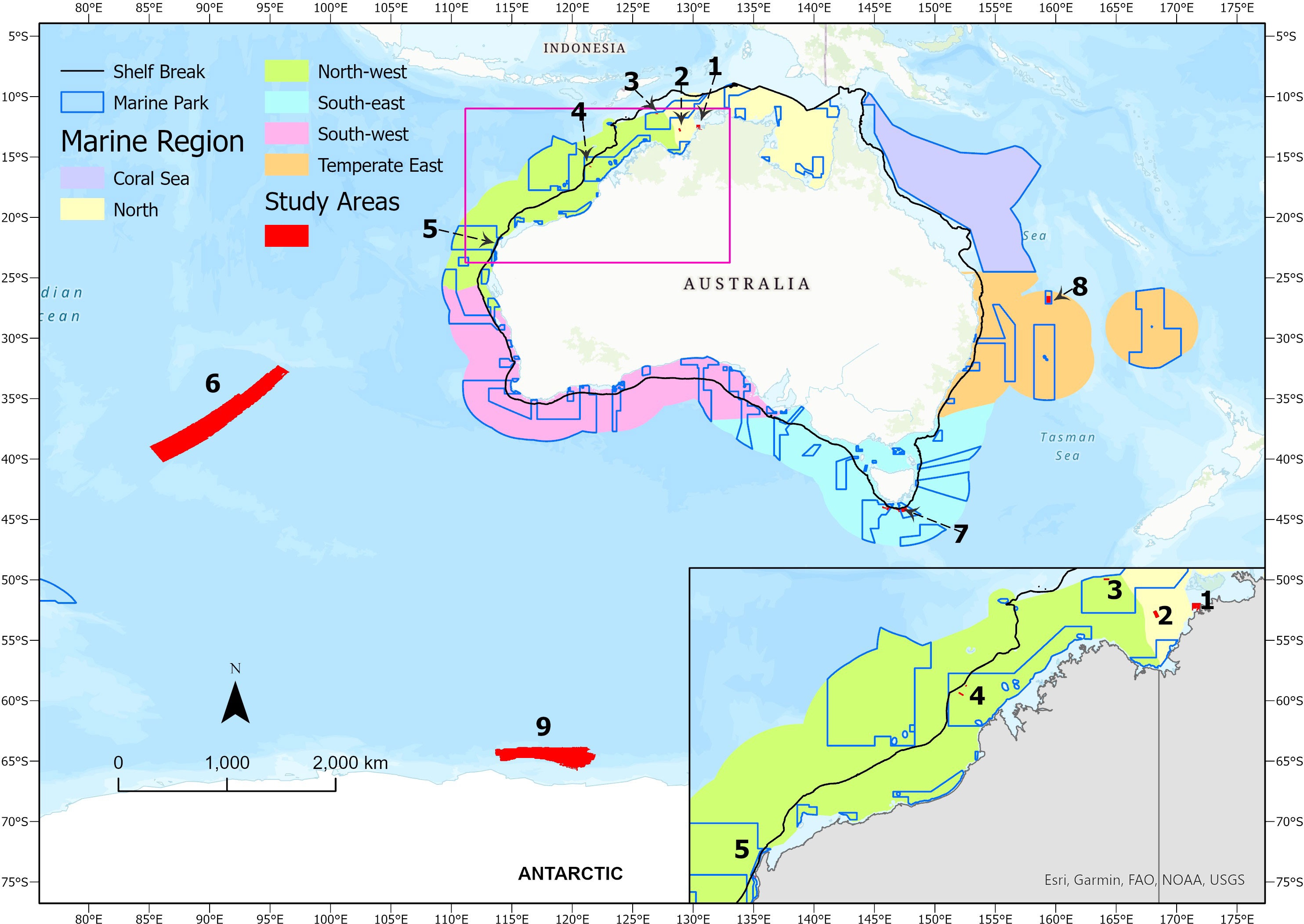
Figure 5 The locations of the nine case study areas, numbered as 1-9. 1: Bynoe Harbour (BH), 2: Bonaparte Shelf (BS), 3: Bonaparte Basin (BB), 4: Leveque Shelf (LS), 5: Point Cloates Shelf (PCS), 6: Broken Ridge (BR), 7: Tasmanian Seamounts (TS), 8: Gifford Seamounts (GS), 9: Sabrina Slope (SS).

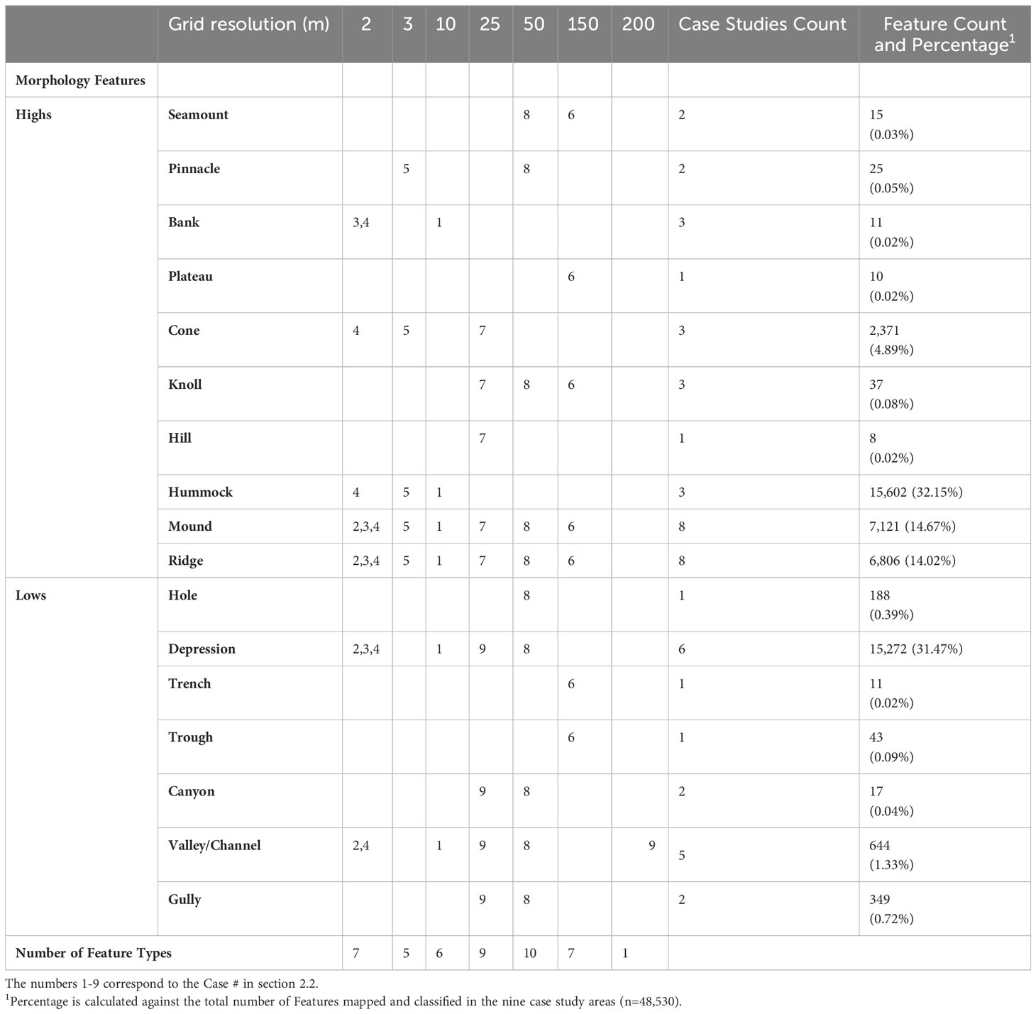
Table 5 Bathymetry grid resolutions and morphology features of the nine case study areas.

Case Study #1: Bynoe Harbour (centred at 12.44° S, 130.43° E) is a tropical estuary located on the northern coast of Australia (Figure 5; Table S1). The area includes Bynoe Harbour and the adjacent shallow shelf with water depths less than 50 m (Siwabessy et al., 2016; Nicholas et al., 2019; Table S1). The multibeam bathymetry dataset was acquired in 2016 using a Kongsberg EM2040C echosounder by Geoscience Australia (GA), the Australian Institute of Marine Science (AIMS) and the Department of Environment and Natural Resources within the Northern Territory Government during a marine survey (GA4452/SOL6432) (Siwabessy et al., 2016). The bathymetry dataset was processed using Caris HIPS/SIPS v8.1 and gridded at 10 m spatial resolution (Figure 6A; Table 5; https://ecat.ga.gov.au/geonetwork/srv/eng/catalog.search#/metadata/144556). Nicholas et al. (2019) found that ridges, hummocks, depressions and channels characterise the area.

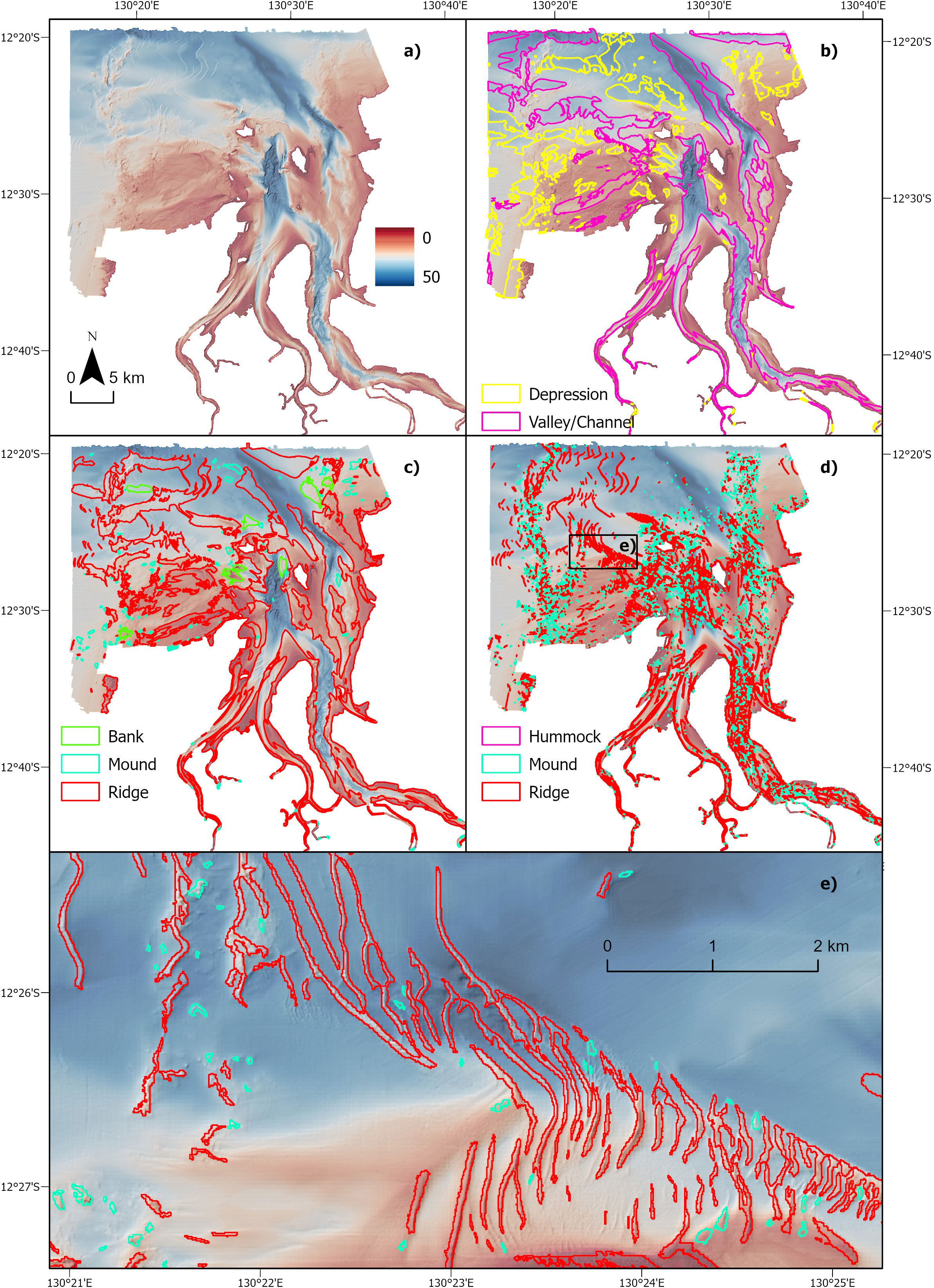
Figure 6 Bynoe Harbour (BH) case study. (A) multibeam bathymetric data; (B) broad scale bathymetric low Features mapped using the TPI tool; (C) broad scale bathymetric high Features mapped using the TPI tool; (D) fine-medium scale bathymetric high Features mapped using the TPI tool; (E) fine-medium scale bathymetric high Features at a sub-area indicated on d (black rectangle outline).

Case Study #2: Bonaparte Shelf (centred at 12.75° S, 128.90° E) is located within the Joseph Bonaparte Gulf of northern Australia (Figure 5; Table S1; Carroll et al., 2012). The area is on the continental shelf with water depths ranging from 80 m to 110 m (Table S1). The multibeam bathymetry dataset was acquired in 2012 using a Kongsberg EM3002D echosounder by GA and AIMS during a marine survey (GA0335/SOL5463) (Carroll et al., 2012). The bathymetry dataset was processed using Caris HIPS/SIPS v7.1 and gridded at 2 m spatial resolution (Figure S9A; Table 5; Spinoccia, 2012). Carroll et al. (2012) described palaeo-channels, low-relief ridges and pockmark fields that characterise this grid.

Case Study #3: Bonaparte Basin case study area (centred at 11.42° S, 127.0° E) is located within the Oceanic Shoals Marine Park in the Timor Sea (Figure 5; Table S1). The area is situated on the continental shelf, with water depths in the range of 50-185 m (Table S1). The multibeam bathymetry dataset was collected in 2012 using a Kongsberg EM3002D echosounder by GA, AIMS, the University of Western Australia and the Museum and Art Gallery of the Northern Territory during a marine survey (GA0339/SOL5650) (Nichol et al., 2013). The bathymetry dataset was processed using Caris HIPS/SIPS v7.1 and gridded at 2 m spatial resolution (Figure 7A; Table 5; Siwabessy and Picard, 2014). Banks, mounds, terraces and tiny depressions (interpreted as pockmarks) are the typical morphological features observed in this area (Nichol et al., 2013).

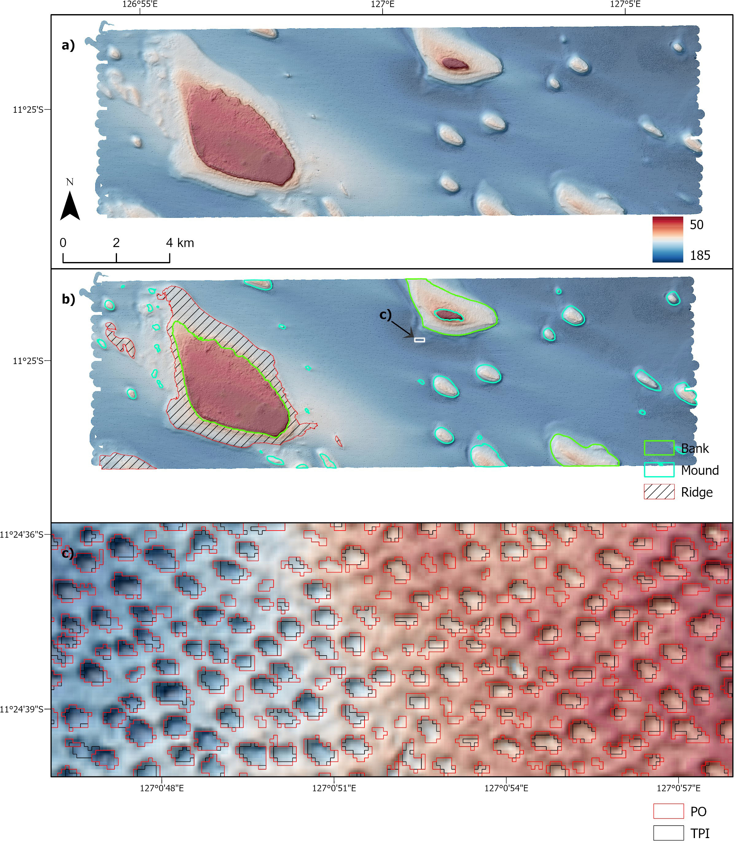
Figure 7 Bonaparte Basin (BB) case study. (A) multibeam bathymetric data; (B) variable scale bathymetric high Features mapped using the TPI tool; (C) very-fine scale bathymetric low Features mapped using the TPI tool and the PO tool at a sub-area indicated on b (white rectangle outline).

Case Study #4: Leveque Shelf has two sub-areas denoted as A1 (centred at 15.8° S, 121.5° E) and A10 (centred at 15.47° S, 121.67° E). The area is located within the Browse Basin offshore northwest Australia in 70 – 110 m water depths (Figure 5; Table S1). The multibeam bathymetry datasets were collected in 2013 using a Kongsberg EM3002 echosounder by GA and AIMS during a marine survey (GA0340/SOL5754) (Picard et al., 2014). The bathymetry datasets were processed using Caris HIPS/SIPS v7.1 and gridded at 2 m spatial resolution (Figures S10A-S10E; Table 5; Picard et al., 2016). The main morphological features observed in this area include banks, terraces, ridges and valleys (Picard et al., 2014).

Case Study #5: Point Cloates Shelf (centred at 22.77° S, 113.66° E) is located within the Ningaloo State Marine Park, offshore Western Australia (Figure 5; Table S1). It lies within the inner and mid continental shelf with water depths less than 85 m (Table S1). The multibeam bathymetry dataset was acquired in 2008 using a Kongsberg EM3002 echosounder by GA and AIMS during a marine survey (SOL4769) (Brooke et al., 2009). The bathymetry dataset was then processed using Caris HIPS/SIPS v6.1 and gridded at 3 m spatial resolution (Figure 8A; Table 5; Spinoccia, 2011). This area contains typical morphological features of banks, mounds, hummocks and ridges (Brooke et al., 2009; Nichol et al., 2012).

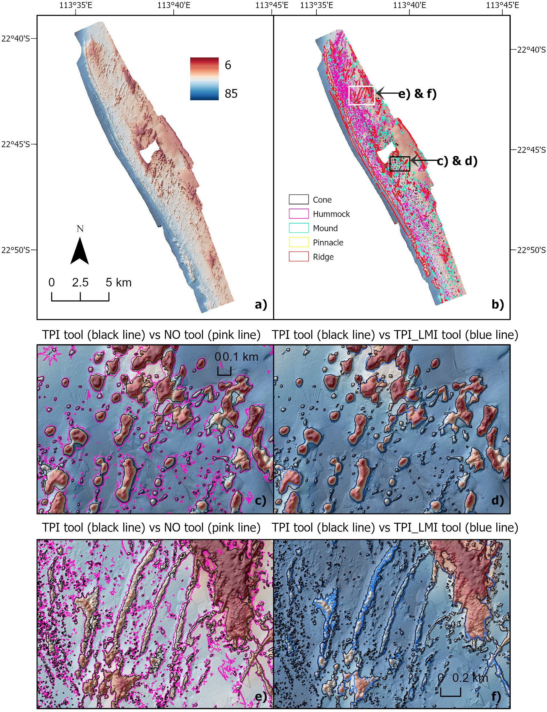
Figure 8 Point Cloates Shelf (PCS) case study. (A) multibeam bathymetry data; (B) fine-medium scale bathymetric high Features mapped using the TPI tool; (C) results of fine-medium scale bathymetric high Features mapped using the TPI tool vs the NO tool at the southern sub-area indicated in b (black rectangle outline); (D) results of fine-medium scale bathymetric high Features mapped using the TPI tool vs the TPI_LMI tool at the southern sub-area; (E) results of fine-medium scale bathymetric high Features mapped using the TPI tool vs the NO tool at the northern sub-area indicated in b (white rectangle outline); (F) results of fine-medium scale bathymetric high Features mapped using the TPI tool vs the TPI_LMI tool at the northern sub-area.

Case Study #6: Broken Ridge (centred at 36.35° S, 91.26° E) is located in the southeastern Indian Ocean, ~1,800 km west of southwest Australia (Figure 5; Table S1; Picard et al., 2018a). Its water depths range from 2,175 m to 5,428 m (Table S1), with abyssal, basin and seamount settings (Harris et al., 2014) (Table S1). The multibeam bathymetry datasets were collected during the MH370 search mission between June 2014 and June 2016 (Picard et al., 2017; Picard et al., 2018a). The datasets were acquired using a Kongsberg EM 302 echosounder on board the MV Fugro Equator, a Kongsberg EM 122 echosounder on board the MV Fugro Supporter and a modified Reson Seabat 7150 echosounder on board the Chinese naval vessel Zhu Kezhen. The bathymetry datasets were then processed using Caris HIPS/SIPS v7.1 and gridded at 150 m spatial resolution (Figure S11A; Table 5; Spinoccia, 2017). Picard et al. (2018a) observed and mapped ridges, knolls, hills, seamounts, plateaus, valleys and troughs in this area.

Case Study #7: Tasmanian Seamounts (centred at 44.15°S, 146.82°E) are located off the south coast of Tasmania, within and adjacent to the Huon and Tasman Fracture marine parks (Figure 5; Table S1; Althaus et al., 2009). The area has water depths ranging from 150 m to 2,400 m (Table S1), with shelf and slope settings according to Heap and Harris (2008) and Harris et al. (2014) (Table S1). The multibeam bathymetry dataset was collected using a Kongsberg EM 300 echosounder in a RV Southern Surveyor voyage (SS200611) in 2006 (Althaus et al., 2009). The bathymetry dataset was then processed using Caris HIPS/SIPS v7.1 and gridded at 25 m spatial resolution (Figure 9A; Table 5; Williams et al., 2022). Numerous seamount-like (mound) bedforms were observed in this area (Althaus et al., 2009; Williams et al., 2020).

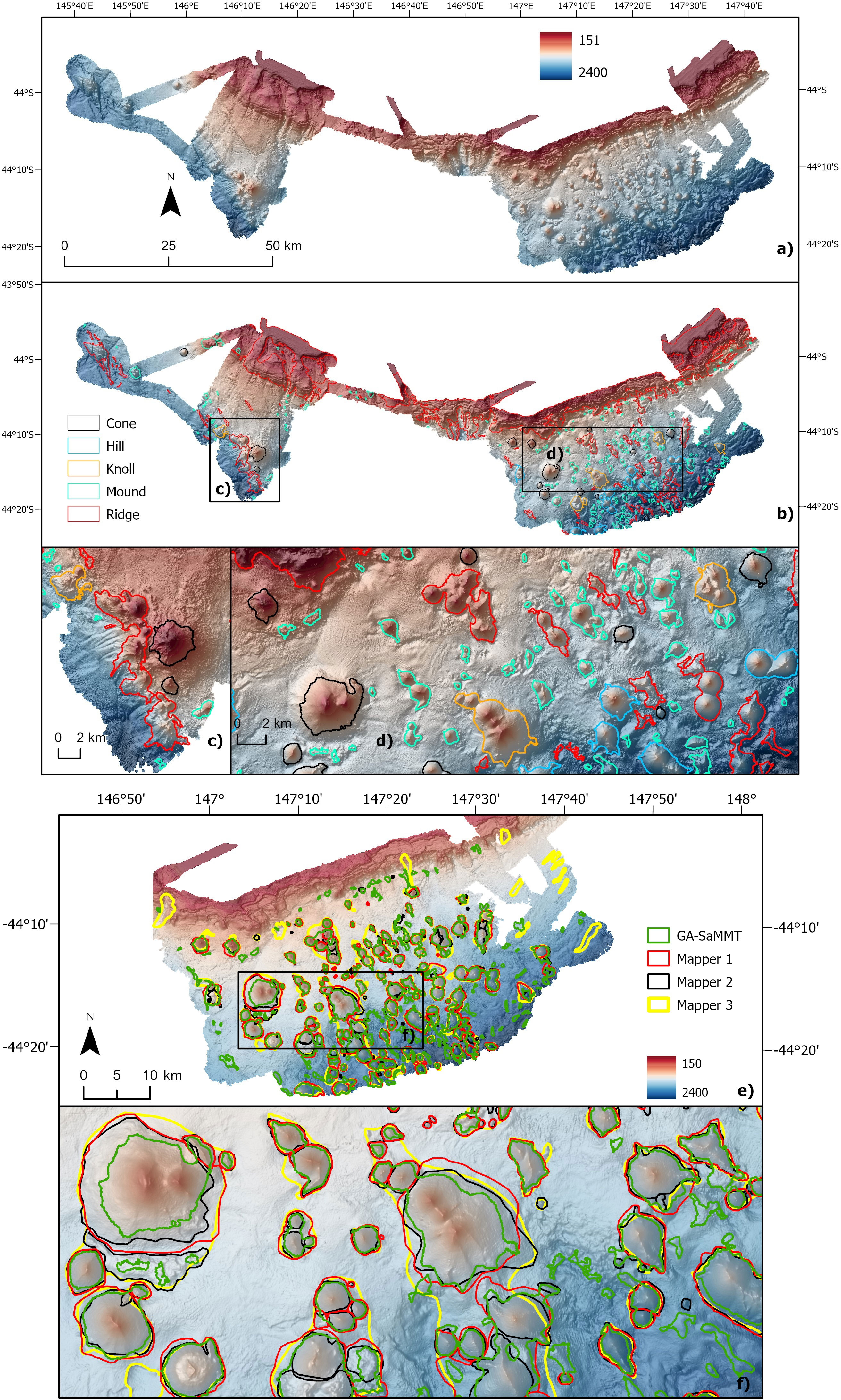
Figure 9 Tasmanian Seamounts (TS) case study; (A) multibeam bathymetry data; (B) variable scale bathymetric high Features mapped using the TPI tool; (C) variable scale bathymetric high Features at the western sub-area indicated on b (black rectangle outline); (D) variable scale bathymetric high Features at the eastern sub-area indicated on b (black rectangle outline); (E) comparison of three manual morphology mapping and GA-SaMMT mapping at a sub-area; (F) the comparison results at an enlarged sub-area indicated on (E) (black rectangle outline).

Case Study #8: Gifford Seamounts (centred at 26.79° S, 146.82° E) are located within the Gifford Marine Park in the Tasman Sea offshore eastern Australia (Figure 5; Table S1). The area covers a large range of water depths from ~250 m to ~3,500 m (Table S1), with the plateau, basin and abyssal settings according to Heap and Harris (2008) and Harris et al. (2014) (Table S1). The multibeam bathymetry datasets were collected in two marine surveys: the GA TAN0713 survey in 2007 (Heap et al., 2009) and the GA and Japan Agency of Marine-Earth Science and Technology survey in 2017 (Nanson et al., 2018). The TAN0713 survey used a Kongsberg EM300 echosounder to acquire the multibeam data; while the JAMSTEC-GA survey used a Kongsberg 12 KHz deep-water multibeam system. The bathymetry datasets were processed using Caris HIPS/SIPS v7.1 and gridded at 50 m spatial resolution (Figure S12A; Table 5; http://dx.doi.org/10.4225/25/5b3174bf2de9b). This area is known to contain two seamounts, with ridges and valley like bedforms on their flat tops and flanks (Heap et al., 2009; Nanson et al., 2018).

Case Study #9: Sabrina Slope (centred at 64.36° S, 117.67° E) is located on the east Antarctic continental slope and rise, seaward of the Budd and Sabrina Coasts of Wilkes Land (Figure 5; Table S1; O’Brien et al., 2020; Post et al., 2020). The area encompasses a wide-range of water depths from ~400 m to ~3,800 m (Table S1), with the shelf, slope, rise and abyssal settings according to Harris et al. (2014) (Table S1). The multibeam bathymetry datasets were collected in 2017 during a RV Investigator survey (IN2017-V01) using Kongsberg EM122 and EM710 echosounders (O’Brien et al., 2020). The bathymetry datasets were then processed using Caris HIPS/SIPS v9.1. Two grids were used in this study. One is a broad-scale grid with 200 m spatial resolution, covering the entire case study area (O’Brien et al., 2020; Figure 10A; Table 5); the other is a small subset gridded at 25 m spatial resolution, covering the upper slope and outer shelf of the case study area (Post et al., 2020; Figure 10C; Table 5). O’Brien et al. (2020) described submarine canyons and valleys characterising the 200 m grid, whereas upper slope gullies and depressions (interpreted as iceberg scours) characterise the 25 m grid situated over the outer shelf (Post et al., 2020).

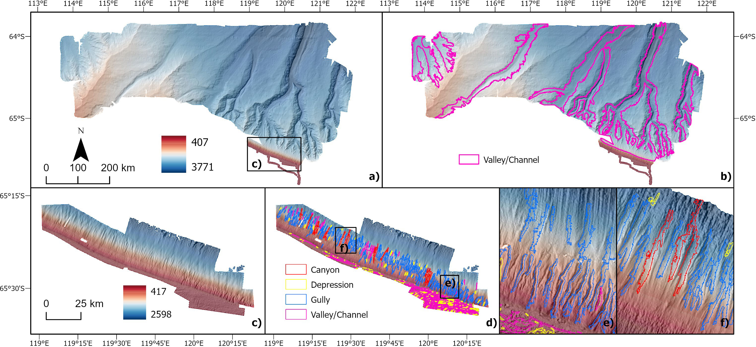
Figure 10 Sabrina Slope (SS) case study; (A) multibeam bathymetry data for the entire area (spatial resolution: 200 m); (B) broad scale bathymetric low Features mapped using the TPI tool; (C) multibeam bathymetry data for the upper-slope and outer-shelf sub area indicated in a (black rectangle outline; spatial resolution: 25 m); (D) fine scale bathymetric low Features mapped using the TPI tool; (E) fine scale bathymetric low features at the western sub-area indicated on d (black rectangle outline); (F) fine scale bathymetric low Features at the eastern sub-area indicated on d (black rectangle outline).

2.3 Evaluating mapping results

In each of these case study areas, there was no existing Morphology Feature map based on the Dove et al. (2020) scheme that could be used as the “ground truth” reference. Instead, GA-SaMMT mapping performance had to be qualitatively assessed by domain experts who visually inspected the results. These qualitative comparisons were also assisted by the visual assessment of the bathymetry and its derived datasets (e.g., Hillshade, slope gradient and TPI), which had also informed the selection of threshold values in GA-SaMMT tools (Huang et al., 2022)

A controlled experiment was also undertaken to provide more quantitative comparisons between manual mapping by domain experts and GA-SaMMT outputs using the ‘TPI Tool Bathymetry High’ for a discrete area. For a portion (2,142 km²) of the Tasman Seamounts case study area (Case #7), which contains pronounced bathymetric high Features (and thus a relatively easy task for manual mapping), mappers visually assessed bathymetry and derived datasets (e.g., Hillshade, Slope, TPI, Contour, etc) and applied the same subset of Dove et al. (2020) Morphology Feature types to delineate and classify the seafloor. The aim of the controlled experiment was to compare relatively subjective manual mapping outputs generated with domain expertise with more objective and repeatable mapping outputs generated from GA-SaMMT. Three experienced practitioners (co-authors on this manuscript) with skills in marine geoscience and GIS data analysis manually digitised and classified polygons of bathymetric high Features following a consistent set of guidelines, including the Dove et al. (2020) nomenclature; a maximum 4 hour time limit; mapping at a scale of 1:25,000; manual vertex placement (i.e., not “streaming mode”). GA-SaMMT were applied to the same dataset using the procedures described in Section 3.7. The manual polygons, attributes and morphology classifications were compared between individual mappers and to GA-SaMMT outputs, and the total length (perimeter), total area, count of feature classes, and count of polygons within each Feature type were quantified and compared. To facilitate a consistent comparison between manual and GA-SaMMT mapping outputs, the manual results were normalised relative to GA-SaMMT result (i.e., GA-SaMMT results comprise 100% of mapped Features against which manual mapping is compared).

3 Results

This section details the results of five case study applications of GA-SaMMT (Bynoe Harbour, Bonaparte Basin, Point Cloates Shelf, Tasmanian Seamounts and Sabrina Slope), which provide diverse representation of physiographic settings across a broad suite of bathymetric spatial scales (Table S1; Table 5). Another four case studies are described briefly here and in more detail within the supplementary materials (Section 1). Specifically, this section describes the application of the mapping tools and their parameters (Table 6) to these diverse datasets, additional spatial analytical steps, and the key mapping results of these case studies.

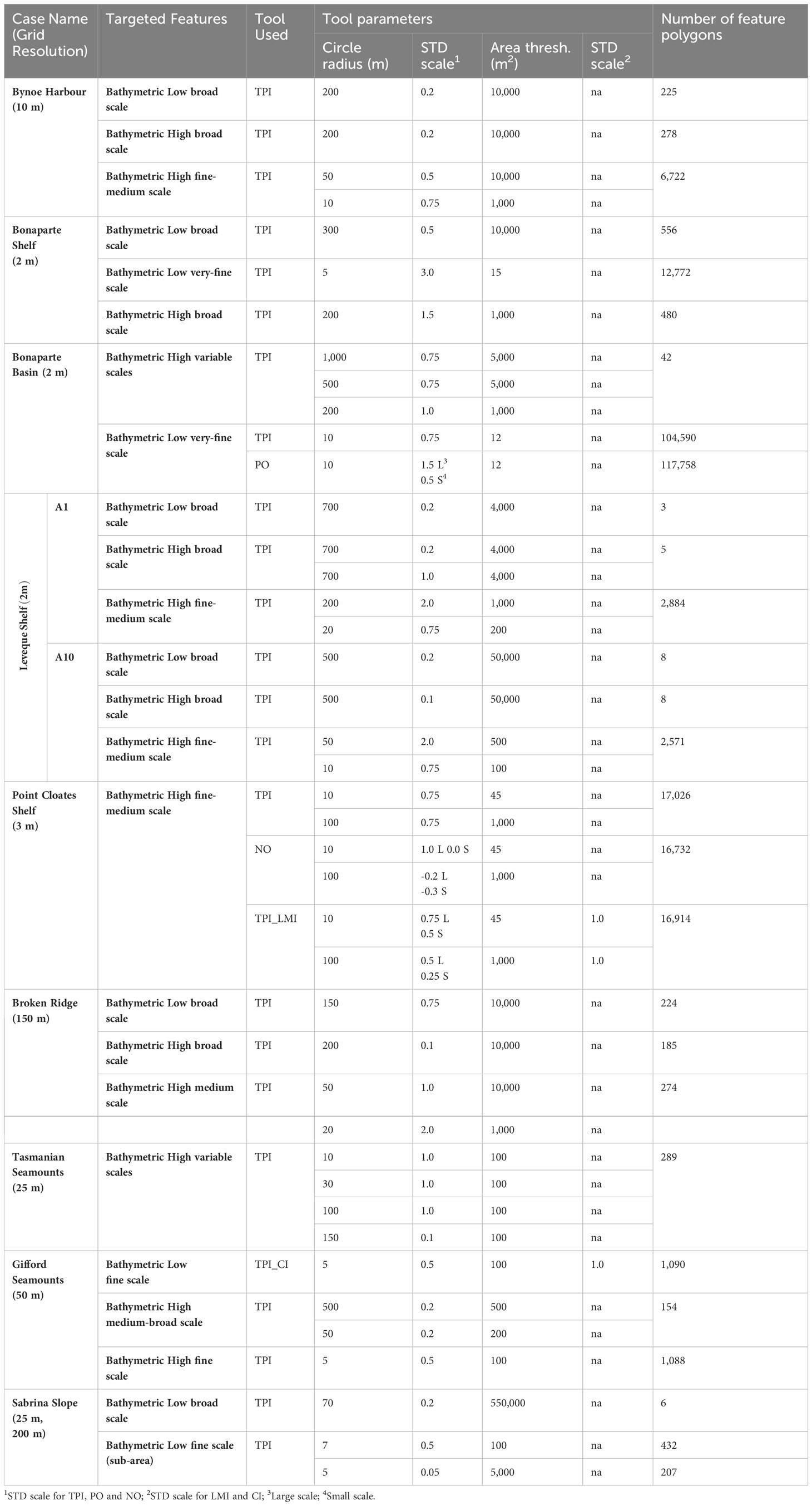
Table 6 GA-SaMMT parameters applied to the mapping of the nine case study areas and the numbers of feature polygons mapped.

3.1 Case #1: Bynoe Harbour

A complex array of ridges, channels and depressions characterise the bathymetry of the Bynoe Harbour dataset (Figure 6A; Nicholas et al., 2019); these were the key targets for testing GA-SaMMT in this case example. Accordingly, we mapped broad scale bathymetric low Features, broad scale bathymetric high Features and fine-medium scale bathymetric high Features (Table 6). The TPI tool was used to map the broad scale bathymetric low Features using the corresponding parameters listed in Table 6. The mapping and subsequent classification using the attributes generated from GA-SaMMT Characterise and Classify tools (Figure 1) resulted in 184 Depressions and 41 Valleys/Channels, respectively (Figure 6B). The two largest channels (>60 km²) were accurately mapped and classified as Valley/Channel. The southern Valley/Channel has two long branches with a head-to-foot length of 28 km and a mean width of 2.5 km; the other on the north-east has a head-to-foot length of ~30 km and a mean width of 2.0 km. The Depressions, which are distributed across the entire area, are generally smaller with a wide range of sizes (0.01 – 15 km²).

The TPI tool was also used to map the broad scale bathymetric high Features using the corresponding parameters listed in Table 6. The mapping and classification resulted in three types of bathymetric high Features: Bank (n=7), Mound (n=130) and Ridge (n=141) (Figure 6C). Ridges are the most dominant broad scale bathymetric high Features, occupying one-third of the total area, and mostly located adjacent to the Valleys/Channels and Depressions. Mounds are also common but generally much smaller, with the largest covering 0.98 km². Banks are few, with their areas ranging from 1.1 km² to 3.8 km².

To map the fine-medium scale bathymetric high Features, we used the TPI tool with the corresponding parameters listed in Table 6, and with analytical steps specified in Table S2. These steps effectively combined the fine scale bathymetric high Features with the medium scale bathymetric high Features that overlap broad scale bathymetric low Features. The mapping and classification resulted in three types of bathymetric high Features: Hummock (n=105), Mound (n=4,142) and Ridge (n=2,475) (Figure 6D). The fine-medium scale Ridges that are prevalent in Bynoe Harbour (Figure 6D) have been interpreted as sediment Ridges (Nicholas et al., 2019). The lengths (measured by the sLength attribute) of these Ridges range from 50 m to ~9 km (mean 491 ± 669 m) and display a wide range of orientations that indicate complex seabed hydrodynamics. However, 40% of mapped ridges are in the north-south orientation, indicating a more dominant East-West seabed current direction. Small Mounds are also prevalent in this area, with sizes less than 0.15 km². As shown in Figure 6E, the boundaries of these fine scale Ridges have been accurately mapped, which demonstrates the satisfactory performance of GA-SaMMT for this case study.

3.2 Case #2: Bonaparte Shelf

In this case study, the broad scale mapping using the TPI tool (Table 6) and the subsequent classification resulted in three types of bathymetric low Features: Depression (n=504), Hole (n=2) and Valley/Channel (n=50) (Figure S9B). The very-fine scale mapping using the TPI tool (Table 6) and the subsequent classification also yielded three types of bathymetric low Features: Depression (n=12,563), Hole (n=95) and Valley/Channel (n=114) (Figure S9C). For bathymetric high features, the broad scale mapping using the TPI tool (Table 6) and the classification resulted in two types of Features: Mound (n=422) and Ridge (n=58) (Figure S9D). The detailed results are provided in section 1.1 of the Supplementary Material.

3.3 Case #3: Bonaparte Basin

The Bonaparte Basin case study aimed to map bathymetric high Features and very-fine scale bathymetric low Features that characterise the dataset (Figure 7A; Table 6), including banks, mounds and depressions reported in Nichol et al. (2013). We used the TPI tool to map the bathymetric high Features using the corresponding parameters listed in Table 6. In this area, there are bathymetric high Features of various scales, not overlapping with each other (Figure 7A). Thus, we attempted to generate a single map of bathymetric high Features using the processing steps detailed in Table S2. Steps 2-4 effectively generated a donut-like feature surrounding the largest rise-up feature; while steps 7 and 9 generated another donut like feature surrounding another rise-up feature.

The resultant map shows three types of bathymetric high Features: Bank (n=3), Mound (n=35) and Ridge (n=4) (Figure 7B). Most of the bathymetric high Features in the area were classified as Mound, which range in area from 0.003 km² to 0.79 km² (mean 0.15 ± 0.19 km²) and 0.5 to 25.3 m in feature height (measured by the dRange attribute) (mean: 8.8 ± 8.3 m). The three Banks are larger features (2.0 – 10.3 km²) with the largest Bank rising to 26.8 m feature height. The four Ridges have variable sizes (0.036 – 8.5 km²). The largest Ridge (8.5 km²) is the donut-like feature surrounding the largest Bank, which should be more appropriately classified as a Terrace according to the morphology scheme of Dove et al. (2020). The other smaller donut-like feature is also a Terrace despite being classified as a Bank in this case study. Note that the current version of GA-SaMMT has not implemented a classification rule for Terrace for the reason presented in section 2.1.1.

We applied both the TPI tool and the Openness Tool (denoted as PO tool in Table 6) separately to map the very-fine scale bathymetric low Features (Table 6). Both tools use the same Circle Radius of 10 cells and other associated parameters (Table 6). The TPI tool and the PO tool resulted in a total of 104,590 and 117,758 features, respectively. These widespread very-fine scale features in this area are very small in size, with the majority of them <200 m² and have previously been interpreted as pockmarks (Nichol et al., 2013). The enlarged map shown in Figure 7C revealed that, in general, both tools were able to reliably map these very-fine scale bathymetric low Features. For most of these features, however, the boundaries mapped by the TPI tool and the PO tool are slightly different. Subsequently, we randomly selected 1,000 of these very-fine scale bathymetric low Features from those resulting from the PO tool for the characterisation and classification steps. The classification result revealed that the vast majority of these features (e.g., 985 out of 1,000) were classified as Depression as expected.

3.4 Case #4: Leveque Shelf

In this case study, for the A1 sub-area, the three largest broad scale bathymetric low Features mapped using the TPI tool (Table 6) and subsequently classified include two Valleys/Channels and one Depression (Figure S10B). The fine-medium scale mapping and classification revealed three types of bathymetric high Features: Hummock (n=1,482), Mound (n=521) and Ridge (n=881) (Table 6; Figure S10C). For the A10 sub-area, the broad scale mapping and classification resulted in two types of bathymetric low Features: Depression (n=5) and Valley/Channel (n=3) (Table 6; Figure S10F). The fine-medium scale mapping and classification resulted in four types of bathymetric high Features: Cone (n=1), Hummock (n=1,516), Mound (n=126) and Ridge (n=928) (Table 6; Table S2; Figure S10G). The detailed results are provided in section 1.2 of the Supplementary Material.

3.5 Case #5: Point Cloates Shelf

The Point Cloates Shelf represents an array of fine-medium scale bathymetric high Features (Figure 8A; Table 6), including banks, mounds, hummocks and ridges reported in Brooke et al. (2009) and Nichol et al. (2012). We used the TPI tool, the Negative Openness tool (NO tool) and the TPI_LMI tool to map the bathymetric high Features separately (Table 6).

The TPI tool with two Circle Radiuses was used to map the fine and medium scales of bathymetric high Features separately before they were combined into a single map of fine-medium scale bathymetric high Features (Table 6; Table S2).The same two Circle Radiuses were used in the NO tool to map the bathymetric high Features (Table 6; Table S2). Similarly, for the TPI_LMI tool, we used the same Circle Radiuses to map the bathymetric high Features (Table 6; Table S2). Note that the feature removed in step 3 was generated due to the edge effect of the TPI_LMI tool.

The mapping of the TPI tool, the NO tool and the TPI_LMI tool resulted in 17,026, 16,732 and 16,914 features, respectively (Table 6). In general, all three tools were able to map the complex and numerous bathymetric high Features in this area. There are, however, some important differences. As shown in Figures 8C, E, the results of the NO tool tend to be more liberal in identifying feature boundaries. As a result, some adjacent features were merged as one single feature. The tool was also sensitive to the artefacts in the bathymetry data, which resulted in over-mapping of unreal smaller features. The TPI_LMI tool and the TPI tool yielded similar results in mapping Hummocks and Mounds (Figure 8D). The TPI_LMI tool, however, was inferior in mapping the narrow linear features than the TPI tool (Figure 8F). For example, a linear feature, which was often mapped as one single feature by the TPI tool, was mapped as a number of shorter features by the TPI_LMI tool. Overall, the TPI tool out-performed both the NO tool and the TPI_LMI tool in this complex case study, as demonstrated in Figures 8C–F.

The classification results of the TPI tool show five types of bathymetric high Features (Figure 8B): Cone (n=2,355), Hummock (n=12,499), Mound (n=1,215), Pinnacle (n=10) and Ridge (n=947). Cones and Hummocks are widespread small features in this area (Figure 8B). They are similar in size, with a mean area of 313 ± 660 m² for cones and 232 ± 205 m² for hummocks, respectively. They are also similar in feature height, with a mean of 2.1 ± 1.8 m for Cones and 1.4 ± 0.8 m for Hummocks. The Mounds, which are larger (mean: 5,196 ± 14,331 m²) and higher (mean: 5.9 ± 3.3 m) than Cones and Hummocks, are also distributed widely. Ridge is another widespread bathymetric high Feature in this area. They are very variable in sinuous length (15 m to 14 km; mean: 166 ± 667 m) and variable in feature height (0 – 35 m; mean: 3.5 ± 4.4 m). The longer Ridges are along the western edge of the area, with a northwest orientation (Figure 8B). Some other prominent Ridges are located on the northern part of this area, with a northeast orientation (Figures 8B, E, F).

3.6 Case #6: Broken Ridge

In this case study, the broad scale mapping and subsequent classification resulted in five types of bathymetric low Features: Depression (n=92), Hole (n=4), Trench (n=11), Trough (n=43) and Valley/Channel (n=74) (Table 6; Figure S11B). For the bathymetric highs, the broad scale mapping and subsequent classification resulted in five types of Features: Knoll (n=7), Mound (n=15), Plateau (n=9), Ridge (n=151) and Seamount (n=3) (Table 6; Table S2; Figure S11C). The medium scale mapping and subsequent classification resulted in five types of bathymetric high Features: Knoll (n=24), Mound (n=42), Plateau (n=1), Ridge (n=197) and Seamount (n=10) (Table 6; Table S2; Figure S11D). The detailed results are provided in section 1.3 of the Supplementary Material.

3.7 Case #7: Tasmanian Seamounts

The Tasmanian Seamounts are extant volcanic features that characterise part of the Huon and Tasman Fracture marine parks within Australia’s South-East Marine Region, and provide important habitat for deep-sea coral reefs communities (Williams et al., 2020). This case example sought to map the extent of these numerous bathymetric high Features of variable scales (Figure 9A) using the TPI tool (Table 6) and the analytical steps listed in Table S2 to obtain a single set of bathymetric high Features. Note that step 2 effectively selected the broad scale features on the northern edge (continental slope) of the case study area. Steps 9&10 identified the bottom portions of the bathymetric high Features. As a result, steps 11&12 effectively extended the extent of individual bathymetric high Features further downslope.

The mapping and classification resulted in five types of bathymetric high Features: Cone (n=15), Hill (n=8), Knoll (n=5), Mound (n=161) and Ridge (n=100) (Figure 9B). None of these bathymetric high Features was classified as Seamount because their feature heights are <1,000 m. The Ridges are the most widespread bathymetric high Features in this area. They have variable areas (0.1 – 310 km²; mean: 8.0 ± 38.7 km²), variable lengths (0.8 – 108 km; mean: 4.9 ± 13.2 km) and variable feature heights (11 – 1,235 m; mean: 186 ± 246 m). Most of them are relatively steep in gradient (mean: 11.0° ± 5.5°). The Mounds are also widely distributed and tend to have small areas (mean: 0.6 ± 1.0 km²), with a mean height of 133 ± 122 m and a mean gradient of 14° ± 9°. Among the Knolls, Hills and Cones, the Knolls tend to be the largest in size (mean: 7.7 ± 3.6 km²), followed by the Hills (mean: 5.8 ± 3.1 km²) and the Cones (mean: 3.4 ± 3.6 km²). The Knolls and Hills have similar feature heights (mean: 605 ± 62 m and mean: 693 ± 133 m, respectively), which are larger than those of the Cones (mean: 417 ± 110 m). These three types of features have also similarly steep gradients (mean: 20.1° ± 3.4° for the Knolls, mean: 23.7° ± 3.8° for the Hills and mean: 23.3° ± 5.2° for the Cones). The enlarged images shown in Figures 9C, D indicate the mapping using the TPI tool performed well in delineating the boundaries of these Knolls, Hills, Mounds and Ridges.

3.8 Case #8: Gifford Seamounts

In this case study, the fine scale mapping using the TPI_CI tool (Table 6) and the subsequent classification resulted in five types of bathymetric low Features: Canyon (n=6), Depression (n=583), Gully (n=197), Hole (n=81) and Valley/Channel (n=223) (Figure S12B).The medium-broad scale mapping using the TPI tool (Tables 6, S2) and the subsequent classification resulted in three types of bathymetric high Features: Mound (n=81), Ridge (n=71) and Seamount (n=2) (Figure S12C). The fine scale mapping using the TPI tool (Tables 6, S2) and subsequent classification resulted in four types of bathymetric high Features: Knoll (n=1), Mound (n=230), Pinnacle (n=15) and Ridge (n=842) (Figure S12D). The detailed results are provided in section 1.4 of the Supplementary Material.

3.9 Case #9: Sabrina Slope

The Sabrina Slope area is characterised by abundant valleys, channels and gullies (Figures 10A, C; O’Brien et al., 2020; Post et al., 2020). This case example aimed to capture these broad scale bathymetric low Features for the entire case study area (Figure 10A), and the fine scale bathymetric low Features on a small upper-slope and outer-shelf sub-area (Figure 10C). The broad scale bathymetric low Features were mapped using the TPI tool with a Circle Radius of 70 cells and the associated parameters listed in Table 6. The mapping of the broad scale bathymetric low Features resulted in six features whose boundaries were accurately delineated (Figure 10B). These six features were subsequently all classified as Valley/Channel (Figure 10B). These are very large features with areas ranging from 679 km² to 4,929 km² (mean: 2,223 ± 1,619 km²). They are also long features with sinuous lengths ranging from 88 km to 350 km (mean: 215 ± 105 km). Although five out of the six features have head-to-foot depth ranges greater than 600 m, these are relatively flat features as indicated by their segment slope gradients of 0.35° – 0.77° and very large mean width-to-thickness ratios (mean: 236 ± 932). Consequently, they were classified as Valley/Channel according to the classification rule derived from the definitions of Dove et al. (2020) (Figures 4B, S8B). It should be noted that O’Brien et al. (2020) classified these features as submarine canyons, consistent with the broader definition of the IHO (2019), and accepted as such by the IHO-IOC GEBCO Sub-Committee on Undersea Feature Names (SCUFN) in 2020. O’Brien et al. (2020) differentiated valley from canyon based on the much larger width-to-depth ratio for a valley. In this case study, the equivalent attribute of width-to-thickness ratio is indeed quite large for all of these six broad scale features.

To map the fine scale bathymetry low Features in the sub-area, we used the TPI tool with the associated parameters and steps listed in Table 6 and Table S2. The mapping and classification resulted in four types of bathymetric low Features: Canyon (n=11), Depression (n=355), Gully (n=152) and Valley/Channel (n=121) (Figure 10D). The Valleys/Channels have two clear groups. One larger group of Valleys/Channels is located on the outer shelf and these have approximately east-west or southeast-northwest orientations. These Features have quite small head-to-foot depth ranges (mean: 5.8 ± 5.6 m) and were previously interpreted as iceberg scour marks (Post et al., 2020). The other much smaller group of Valleys/Channels are located on the main upper-slope area and are orientated approximately northeast-southwest. They have a much larger head-to-foot depth ranges (mean: 288 ± 133 m). The Gullies are distributed across the entire upper-slope and outer-shelf sub-area and are also generally orientated northeast-southwest. Their sinuous lengths range from 1.0 km to 6.7 km (mean: 2.5 ± 1.3 km), with mean widths ranging from 80 m to 433 m (mean: 175 ± 63 m). They have head-to-foot depth ranges vary from 145 m to 1,317 m (mean: 501 ± 270 m). These Gullies are relatively steep in gradient, with a mean segment slope of 10.5° ± 2.0° and a mean gradient of 13.8° ± 2.1°. A small number of Features among the Gullies and Valleys/Channels were classified as Canyon (Figure 10D). These Canyons tend to be longer (mean: 4.8 ± 1.2 km in sinuous length), wider (mean: 288 ± 145 m in mean width), and larger in head-to-foot depth range (mean: 956 ± 196 m) than the Gullies. However, they have similar slope gradient (mean: 10.6° ± 1.2° in mean segment slope; mean: 13.8° ± 1.2° in mean gradient) as the Gullies. The Depressions are small (mean: 0.04 ± 0.06 km²) and are located mostly among the elongated iceberg scour marks (Figure 10D). They are also relatively gentle in slope gradient (mean: 3.8° ± 3.0° in mean gradient). The enlargedmaps of Figures 10E, F show that the boundaries of the Gullies, Valleys/Channels and Canyons were mapped with reasonable accuracy.

3.10 Manual mapping and semi-automated mapping comparison

The results of the controlled experiment comparing the manual mapping and the semi-automated mapping in a sub-area of the Tasmanian Seamounts case study area are summarised in Table 7 and illustrated in Figures 9E, F. All three manual mappers chose a similar suite of bathymetry derivatives (hillshade and slope gradient) to inform their mapping of polygon outline boundaries. Contour and curvature were also used by different individuals. The ‘TPI Tool Bathymetry High’ in GA-SaMMT, however, utilised only TPI.

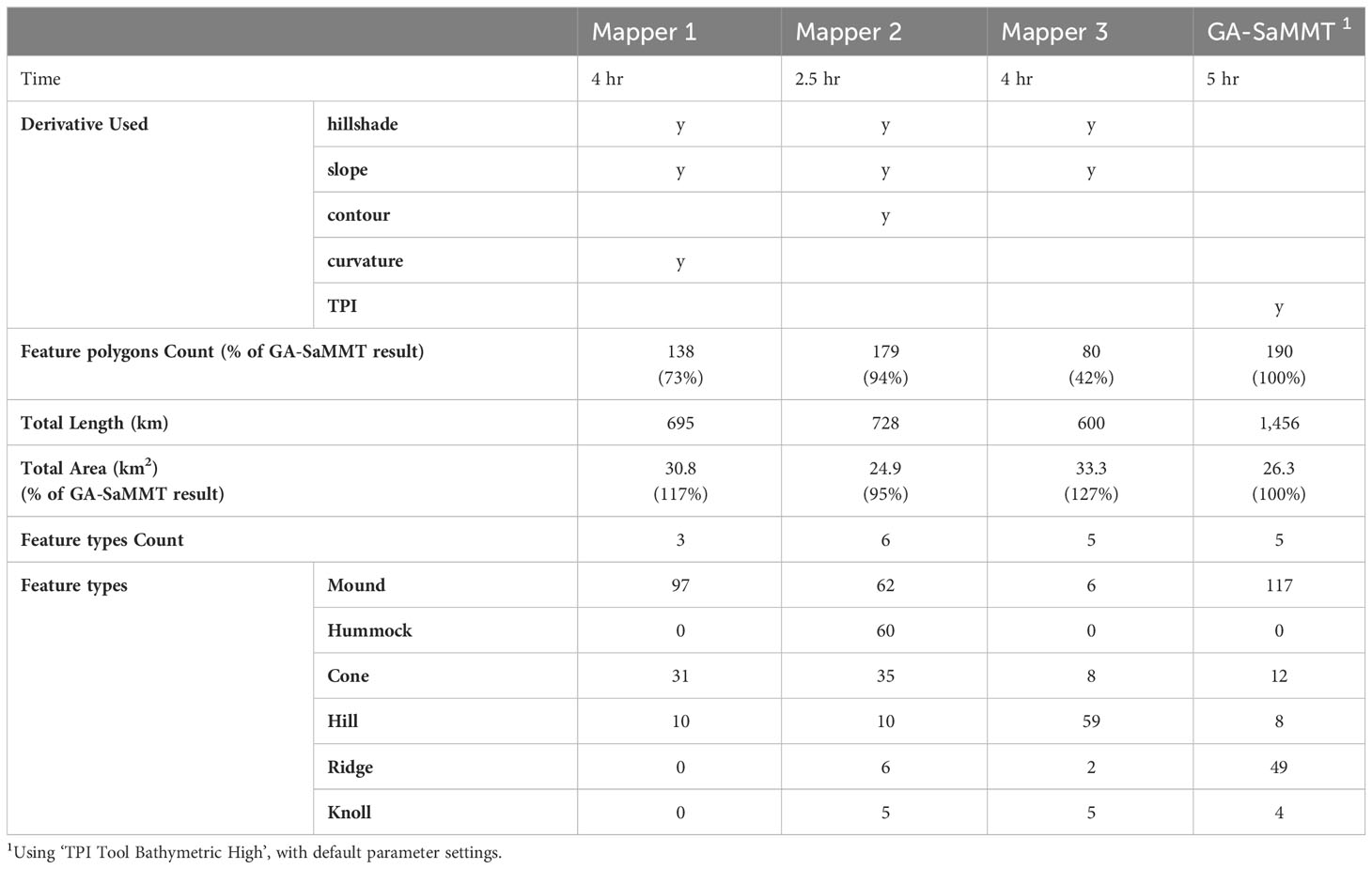
Table 7 Summary of the comparison between manual mappers and GA-SaMMT outputs.

A visual comparison of polygon boundary footprints relative to the underlying seabed features demonstrates some variability in the treatment of adjoined features, for both the GA-SaMMT and between manual mappers. Some mappers lumped while others split adjoined features. GA-SaMMT sometimes adjoined adjacent features as well. Notably, GA-SaMMT tended to underestimate polygon footprints by conservatively interpreting the break-in-slope between bathymetric high features and the planar seabed.

The quantitative results revealed considerable variability between the three manual mappers and GA-SaMMT approach. The key differences were: (1) the total number of feature polygons generated (manual n = 138, 179 and 80 vs GA-SaMMT n = 190); (2) the area they cover (as a percentage of GA-SaMMT 100%: manual mapping covered 117%, 95% and 127%); and (3) the number of Morphology Feature types attributed to individual feature polygons (manual n = 3, 6 and 5 vs GA-SaMMT n = 5). Indeed, Mapper 3 defined only 6 Mounds compared to 97 and 62 from Mappers 1 and 2, respectively. Mapper 3 also mapped far fewer Cones than the other two mappers. However, Mapper 3 mapped many more Hills than the other two mappers. In contrast, Mapper 2 mapped 60 Hummocks while none of these were identified by Mappers 1 and 3. GA-SaMMT mapped 190 feature polygons and 5 Feature types, with many more Ridges and Mounds, and fewer Hills than any of the manual mappers. Some of these differences may be attributed to the manual mapping guideline which instructed mappers to use the definitions described in Dove et al. (2020), however, many of those Morphology Feature definitions are qualitative descriptions rather than quantitative threshold values implemented by the rule-based GA-SaMMT (Figures 4, S8). In addition, the total length (perimeter) and the total area of feature polygons among the manual and semi-automated mappings showed some variations but they were all within an order of magnitude.

4 Discussion

A key objective of seabed morphological mapping is the ability to objectively derive maps that support the quantitative analysis and interpretation of seabed environments from their geomorphic character. The rule-based, semi-automated mapping method tested here for a diversity of seabed environments supports this aim through a technique that allows a structured approach to mapping seabed geomorphology. Collectively, the nine case examples resolved ten types of bathymetric high Features and eight types of bathymetric low Features across a wide range of spatial resolutions, with a total Feature count of 32,006 and 16,524, respectively (Table 5). Additionally, this mapping method can be applied at multiple spatial scales in situations where the data supports the co-existence of features of multiple scales and feature-on-feature mapping. From our case examples, the two medium-resolution bathymetric grids (25 m and 50 m) were able to resolve nine and ten bathymetric high and low Feature types, respectively; while the bathymetric grid with the coarsest spatial resolution (200 m) was only able to resolve one Feature type (Table 5). Of the total number of mapped and classified Features, over 97% are classified as Hummocks (32%), Depressions (31%), Mounds (15%), Ridges (14%) and Cones (5%) (Table 5). Hummocks and most Depressions mapped in this study are primarily fine scale features that have developed in great numbers, many of which are interpreted as vast fields of pockmarks. The common occurrence of Mounds and Ridges in this study (Table 5) is mainly due to the fact that they have the least constrained bathymetric high definitions (Table 1).

In this study, we compared the performance of the TPI tool and the PO tool in mapping very-fine scale bathymetric low Features in the Bonaparte Basin area (Figure 7C). We also compared the performance of the TPI tool, the NO tool and the TPI_LMI tool in mapping fine-medium scale bathymetric high Features in the Point Cloates Shelf area (Figures 8C–F). However, based only on these two comparison studies, we are not able to judge the performance of one tool against another; more comprehensive comparison study would be required for that purpose. In this study, based on the mapping results, we have instead demonstrated that these mapping tools individually perform well in the presented case studies.

One key advantage of using the semi-automated tools (GA-SaMMT), compared to other semi-automated methods (e.g., Lundblad et al., 2006; Lanier et al., 2007; Erdey-Heydorn, 2008; Zieger et al., 2009; Micallef et al., 2012; Harris et al., 2014; O’Brien et al., 2015; Jerosch et al., 2016; Picard et al., 2018b; Hebbeln et al., 2019; Lavagnino et al., 2020; Sowers et al., 2020; Weinstein et al., 2021), is their ability to generate a large number of metrics (Tables 2–4) to comprehensively characterise individual features from a range of aspects. These metrics are invaluable for post-mapping analysis, for their geomorphic interpretation and classification (e.g., Nanson et al., 2023). They also provide valuable insights into their habitat potential for various marine biota (e.g., McArthur et al., 2010; Huang et al., 2011). In the following sections we provide two examples of such post-mapping analyses to demonstrate the value of these metrics for providing further insights into the bathymetric high and low Features mapped in this study.

4.1 Inter-feature variability of bathymetric high features

Six metrics were used to explore broad differences between the ten types of bathymetric high Features mapped across the nine case study areas (Figure 11). Among these six metrics, Area and depthRange have been used in the classification rules of some bathymetric high Features (Figure 4A). The boxplots indicate that:

● While the classification rule (depthRange ≥ 1000 m; Figure 4A) dictates that Seamounts are high-relief (Figure 11D), Figures 11A, C also reveals that they are large seabed Features that often occur in deeper water, the restriction of smaller and low-relief Hummocks, Mounds, Banks, Ridges and Cones to shallower water is independent of these rules;

● Ridges and Cones have the most and the least complex polygon shape, respectively (Figure 11B);

● Hills and Pinnacles were found to be topographically steep features (meanGradient > 20°); while most Banks and Mounds are relatively flat features (meanGradient < 5°) (Figure 11E);

● While the classification rule (Area ≥ 100 km²; Figure 4A) dictates that Plateaus are overall the largest features (Figure 11A), Figure 11C reveals that, independent of the rule, they occur in the deepest water; and

● Mounds and Ridges have the greatest variation in all six attributes (Figure 11). This is mainly because these two Feature types have the least restrained definitions among the ten bathymetric high Feature types (Table 1). The broad geometric variations of mapped Ridges are also partly due to the relatively small lwRatio threshold value of 5.0 (e.g., the default value) used in this study (Figure 4A). It follows that these two Feature types clearly represent a variety of seabed environments and processes such that additional geometric analyses and data (e.g. sub-bottom profiles, physical samples) are required to support further interpretation.

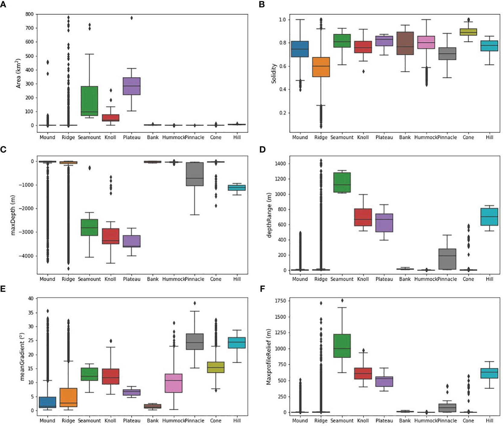
Figure 11 Different characteristics of the 10 bathymetric high Features across the case study areas; (A) Feature area; (B) Solidity; (C) Maximum (the shallowest) water depth within the feature; (D) Feature depth range (height); (E) Feature mean gradient; (F) Maximum profile relief (in elevation) of the feature. Note that the number of features for each Feature type is listed in Table 5. Each color box represent the inter-quartile range with the median value marked as the line dividing the box; The upper whisker to the upper quartile line represents the upper 25% data points; the lower quartile line to the lower whisker represents the lower 25% data points; the dots represent outliers which are data points that are outside 1.5 times of the inter-quartile range above the upper quartile and below the lower quartile.

These statistics can also be used to highlight depth bias in Feature mapping as bathymetry grid resolutions are generally negatively correlated with their water depth; smaller-scale Features are likely being underrepresented in deeper-water grids (Picard et al., 2018a). For example, Hummocks (≤ 10 m dRange rule: Figure 4A) might be expected to occur in a broad range of water depths, but were only identified in shallow water (Figure 11C), in finer resolution grids (Table 5).

4.2 Inter-feature variability of individual bathymetric low features

Eight metrics are used to quantify the characteristic differences between the eight bathymetric low Features (Figure 12). Among these eight metrics, lwRatio and hDepth have been used in the classification rules of some bathymetric low Features (Figure 4B). These boxplots indicate that:

● Troughs are much larger than other bathymetric low Features (Figure 12A); this is consistent with their origin being typically influenced by large-scale geological processes such as horst and graben structures and faults;

● Depressions and Holes have the least complex polygon shapes for bathymetric low Feature, likely because they are not elongated features (Table 1) (Figure 12B);

● Canyons are the most elongated features (Figure 12C); as their hfDepthRange must exceed 600 m (Figure 4B), it follows, geometrically, that these features also extend over long distances (high lwRatio);

● Valleys/Channels have higher width-to-thickness ratios than Canyons (Figure 12D), which is broadly consistent with their origin being driven by downslope sediment and fluid transport (e.g., Gibling, 2006; Harris and Whiteway, 2011);

● Troughs and Trenches occur in the deepest water depths (Figure 12E), which is dictated by their classification rules (hDepth ≥ 4000 m; Figure 4B); however, independent from the classification rules, Figure 12E also reveals that the Gullies and Canyons occur in intermediate water depths (500 - 1,500 m), and that Holes and Valley/Channels can occur in a large range of water depths from shallow water to water depth of ~2,500 m (Figure 12E);

● Canyons incise deeper into seabed along the long axis, followed by the gullies (Figure 12F); and

● Gullies and Canyons are steeper features (>15°) than Holes, and other bathymetric low Features (Figure 12G); and Troughs and Trenches have higher cross-sectional profile reliefs (>100 m) than other bathymetric low Features (Figure 12H).

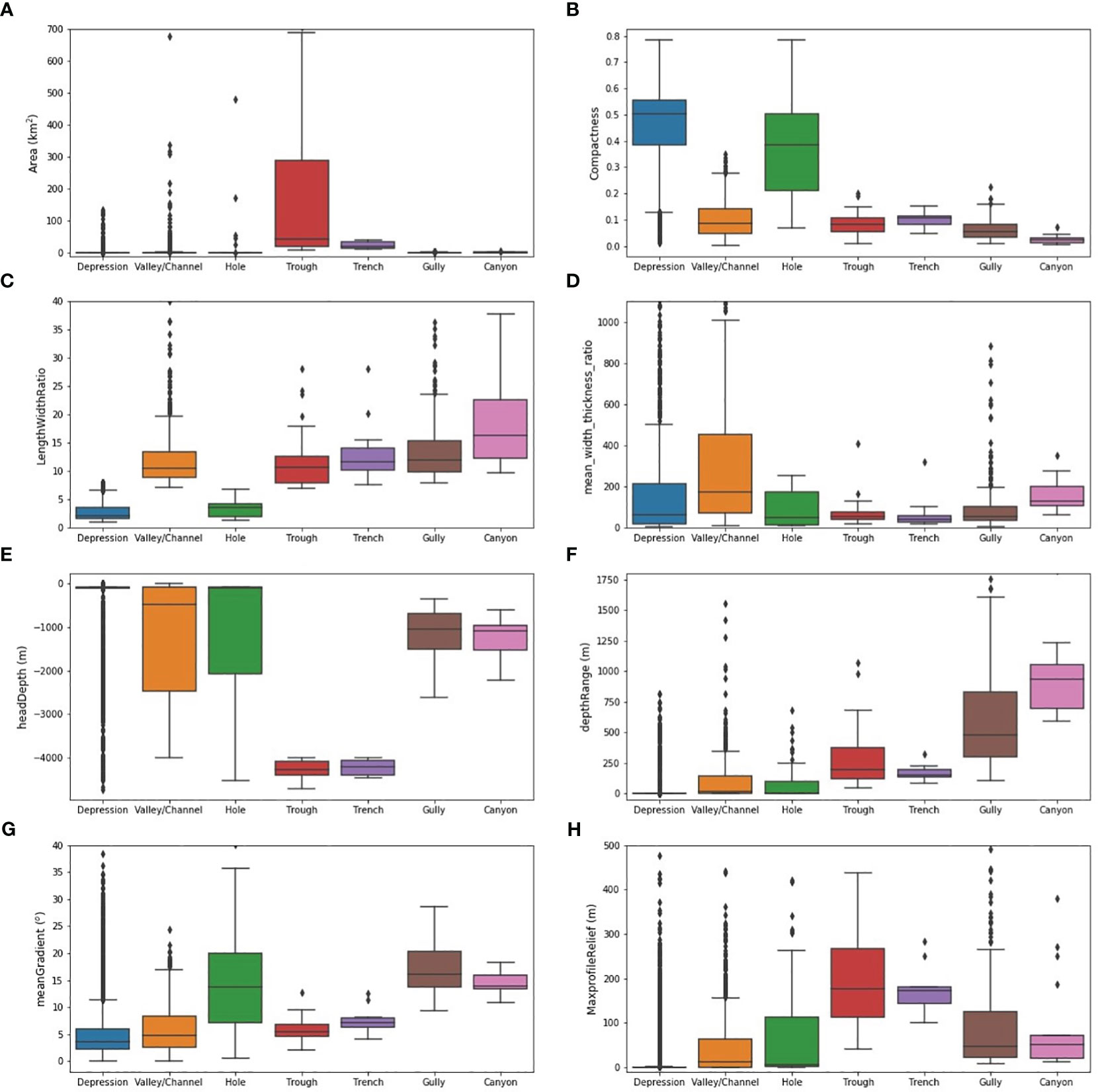
Figure 12 Different characteristics of the eight bathymetric low Features across the case study areas; (A) Feature area; (B) Feature compactness; (C) Feature length to width ratio; (D) Feature mean width-to-thickness-ratio; (E) Water depth at the head of the feature; (F) Feature depth range; (G) Feature mean gradient; (H) Maximum profile relief (in elevation) of the feature. Note that the number of features for each Feature type is listed in Table 5.

Again, although some of the above findings are inherited from their respective classification rules (e.g., regarding Troughs and Trenches as the deepest features), other findings provide additional insights into these Features.

4.3 Limitations of the GA-SaMMT

One limitation of GA-SaMMT is the computing resources required to generate attributes (polygon metrics), particularly since parallel processing has not been implemented in the current version of the software tools. In this study we recorded the time required to generate attributes for the fine-medium scale bathymetric high Features mapped for the A1 sub-area of the Leveque Shelf case study (n=2,884; Figure S10C) and the fine scale bathymetric low Features mapped for the Gifford case study (n=1,090; Figure S12B). To speed-up the tools, for each set of features, we divided them into three equal-number subsets and ran the tools concurrently with each subset. Under the specified computer settings (Intel (R) Core i7-8700 CPU (6 cores), @3.20 GHz, 64 GB RAM), the times required to complete these attribute tools are listed in Table S3. The Add Topographic Attributes Tools required little time to complete (e.g., 0.01 second and 0.04 second per feature, respectively). The Add Shape Attributes High Tool and the Add Profile Attributes High Tool required 2.4 seconds per feature and 9.6 seconds per feature, respectively. The Add Shape Attributes Low Tool and the Add Profile Attributes Low Tool needed 10.8 seconds per feature and 12 seconds per feature, respectively. The four-fold increase in the time required to generate the shape attributes for each bathymetric low Feature compared to that for each bathymetric high Feature is due to the eight extra shape attributes to be calculated (Table 2). For future versions of GA-SaMMT, we intend to examine the coding efficiency and the possibility of parallel processing. However, for the current version and utilising a modern multi-core CPU, we highly recommend sub-setting and concurrent running of datasets to improve the efficiency in the generation of shape and profile attributes for a large number of features.

Another limitation of GA-SaMMT is the expertise required to achieve an optimal mapping result for a mapping application. The semi-automated nature of these tools requires selections of a number of user-defined threshold values. This requirement is particularly challenging for a morphologically complex area that has seabed features of multiple scales. In this study, significant domain knowledge was utilised in the selection of appropriate tool parameters, through iterative applications of GA-SaMMT Map and Classify tools, for each case study. In addition, advanced GIS and spatial analysis skills are required to obtain an optimal mapping result. As shown in this study, our methods employed additional spatial analytical steps to obtain the final sets of the bathymetric high or low Features (Table S2). The mapping results shown in Figures 6–10 and Figures S9-S12 indicate that these seabed morphology maps can also be further improved by conducting additional post-mapping modifications such as editing features’ polygon shapes, merging adjacent features, and splitting a feature into multiple features, etc. In this study, the success of our mapping using GA-SaMMT is attributed to collaborative work in a team of experienced marine geomorphologists and spatial analysts.

The current version of GA-SaMMT are not designed to map all the seabed Feature types defined by Dove et al. (2020). Some 13 out of 31 Feature types cannot be mapped using this version of the tools, for the reasons presented in section 2.1.1. For example, the two Terraces clearly visible in Figure 7A were accurately mapped but were incorrectly classified as a Ridge and a Mound (Figure 7B), likely due to their least restrained definitions (Table 1; Dove et al., 2020) and the corresponding classification rules (Figure 4A). In future versions of GA-SaMMT we will attempt to extend the classification rules to include more of the 13 remaining bathymetric high and low Feature types (greyed in Figure 2). We will also attempt to improve the existing classification rule for Depression to satisfy its definition as a closed-contour bathymetric low Feature (Table 1; Dove et al., 2020).

5 Summary and conclusions

Seabed morphology maps are products critical for interpreting physical, biological and oceanographic processes that operate in the marine environment. They have application across a diversity of users, including engineering, science and policy. The need for tools that support consistent and objective mapping of seabed features is clear. This study developed a number of rule-based, semi-automated GIS tools (GA-SaMMT: Huang et al., 2022) to operationalise the mapping of bathymetric high and bathymetric low seabed Morphological Features, and targeted a subset of common Features defined by Dove et al. (2020). These were developed as Python tools under the widely-used proprietary ArcGIS Pro platform, with user-friendly graphical interfaces and extensive tool tips and metadata, and the source codes are publicly available to users for modification and further development (Huang et al., 2022).

We have tested the utility of these tools across nine case study areas that cover a diverse range of complex bathymetric and physiographic settings (Table S1). Qualitative visual comparisons between the mapping results and the features identified by previous work as being high priority (e.g. in survey reports) indicate that GA-SaMMT can accurately and consistently capture their extents. In our controlled mapping experiment the variations between all three manual mappers (Figures 9E, F; Table 7) highlight the subjectivity of picking feature outlines, even when working at a set mapping scale and using similar bathymetry derivatives to help inform feature boundaries. The variation in manual mapping results further highlight the benefit of objective and repeatable semi-automated approaches such as GA-SaMMT.

We also note the following additional advantages of GA-SaMMT:

● requirement of only a bathymetry grid (preferably derived from high-quality multibeam data) as sole data input;

● the incorporation of domain knowledge via the input of user-defined tool parameters (including the option to retain default parameter settings);

● repeatability and consistency in the mapping outputs when using a consistent set of user-defined tool parameters (or default parameter settings);

● high degree of objectivity;

● flexibility to adapt to individual applications using user-defined tool parameters;

● ability for multi-scale mapping; and

● efficiency in mapping and characterising a large number of seabed Morphology Features.

Another key advantage of GA-SaMMT over other semi-automated methods is the ability of the tools to generate a large number of attributes (Tables 2–4) to quantitatively characterise the Morphology Features. The results of this study clearly indicate that the ten bathymetric high Features and eight bathymetric low Features have distinctly different shapes, topography and cross-sectional profiles (Figures 11, 12).

It should be emphasised that the three-step solution offered by GA-SaMMT (Figure 1) does not require inter-dependency between the first step (GA-SaMMT Map) and the next two steps (GA-SaMMT Characterise and GA-SaMMT Classify). Users have flexibility to map feature polygons using manual or other semi-automated methods suitable for their specific applications and then apply the next two steps to characterise and classify the feature polygons according to Dove et al. (2020) scheme.

In future work we intend to further develop these rule-based, semi-automated tools through their application to further datasets, particularly to enhance their functionalities and efficiency. This will include examining the feasibility of parallel cloud-based processing, the development of new mapping tools (e.g., based on other bathymetry derivatives), and expanding classification tools to incorporate the remaining bathymetric high and low Features defined in Dove et al. (2020). In addition, the availability of the source codes of GA-SaMMT are expected to drive future development/improvement of these semi-automated seabed morphology mapping tools.

Data availability statement

The datasets presented in this study can be found in online repositories. The names of the repository/repositories and accession number(s) can be found below: Bynoe Harbour: https://ecat.ga.gov.au/geonetwork/srv/eng/catalog.search#/metadata/144556; Bonaparte Shelf: https://ecat.ga.gov.au/geonetwork/srv/eng/catalog.search#/metadata/74866; Bonaparte Basin: https://ecat.ga.gov.au/geonetwork/srv/eng/catalog.search#/metadata/79006; Leveque Shelf: https://ecat.ga.gov.au/geonetwork/srv/eng/catalog.search#/metadata/83727; Point Cloates Shelf: https://ecat.ga.gov.au/geonetwork/srv/eng/catalog.search#/metadata/72005; Broken Ridge: https://ecat.ga.gov.au/geonetwork/srv/eng/catalog.search#/metadata/82625; Tasmanian Seamounts: https://doi.org/10.25919/qan1-qj27; Gifford Seamounts: https://ecat.ga.gov.au/geonetwork/srv/eng/catalog.search#/metadata/121193; Sabrina Slope: https://ecat.ga.gov.au/geonetwork/srv/eng/catalog.search#/metadata/144481.

Author contributions

ZH, RN, SN, and AP designed the study. ZH and MW conducted the case studies. MM, MW, and JG conducted the manual mapping experiment. ZH wrote the initial version of the manuscript. All authors contributed to the article and approved the submitted version.

Funding

The open access publishing fee for this paper was kindly provided by Geoscience Australia.

Acknowledgments

We thank the following people for testing the earlier versions of GA-SaMMT: Tina Yang and Larissa Taylor of Geoscience Australia, Riccardo Arosio of University College Cork and Alysha Johnson of University of Wollongong. We also acknowledge numerous GA colleagues and external collaborators who collected and processed, and various funding programs (Commonwealth Environmental Research Facilities Program; National Environmental Research Program; National Environmental Science Program; Offshore Energy Security Program; National Low Emissions Coal Initiative/National CO2 Infrastructure Plan) that supported the acquisition of the multibeam data used in this study. The valuable comments from Tony Nicholas, Kim Picard, Andrew Carroll and Duncan Moore of Geoscience Australia have improved the manuscript. We would like to thank two reviewers for their detailed and constructive comments that have significantly improved this manuscript. This paper is published with permission of the CEO, Geoscience Australia.

Conflict of interest

The authors declare that the research was conducted in the absence of any commercial or financial relationships that could be construed as a potential conflict of interest.

Publisher’s note

All claims expressed in this article are solely those of the authors and do not necessarily represent those of their affiliated organizations, or those of the publisher, the editors and the reviewers. Any product that may be evaluated in this article, or claim that may be made by its manufacturer, is not guaranteed or endorsed by the publisher.

Supplementary material

The Supplementary Material for this article can be found online at: https://www.frontiersin.org/articles/10.3389/fmars.2023.1236788/full#supplementary-material

References

Althaus F., Williams A., Schlacher T. A., Kloser R. J., Green M. A., Barker B. A., et al. (2009). Impacts of bottom trawling on deep-coral ecosystems of seamounts are long-lasting. Mar. Ecol. Prog. Ser. 397, 279–294.
Beaman R. J., Harris P. T. (2005). Bioregionalization of the george V shelf, east Antarctica. Continental Shelf Res. 25, 1657–1691.
Brooke B., Nichol S., Hughes M., McArthur M., Anderson T., Przeslawski R., et al. (2009). Carnarvon Shelf Survey Post-cruise Report. Geoscience Australia, Record . 2009/002 (Geoscience Australia, Canberra)
Carroll A. G., Jorgensen D. C., Siwabessy P. J. W., Jones L. E. A., Sexton M. J., Tran M., et al. (2012). Seabed environments and shallow geology of the Petrel Sub-Basin, northern Australia: SOL5463 (GA0335) - post survey report. Record 2012/66 (Geoscience Australia: Canberra).
Dove D., Bradwell T., Carter G., Cotterill C., Gafeira Goncalves J., Green S., et al. (2016). Seabed geomorphology: a two-part classification system. Br. Geological Survey.
Dove D., Nanson R., Bjarnadóttir L., Guinan J., Gafeira J., Post A., et al. (2020). A two-part seabed geomorphology classification scheme (v.2); Part 1: morphology features glossary. Zenodo. doi: 10.5281/zenodo.4075248
Erdey-Heydorn M. D. (2008). An ArcGIS seabed characterization toolbox developed for investigating benthic habitats. Mar. Geodesy 31, 318–358.
Ferrini V. L., Flood R. D. (2005). A comparison of Rippled Scour Depressions identified with multibeam sonar: Evidence of sediment transport in inner shelf environments. Continental Shelf Res. 25, 1979–1995.
Fisher P., Wood J., Cheng T. (2004). Where is Helvellyn? Fuzziness of multi-scale landscape morphometry. Trans. Institute Br. Geographers 29, 106–128.
Gibling M. (2006). Width and thickness of fluvial channel bodies and valley fills in the geological record: A literature compilation and classification. J. Sedimentary Res. 76, 731–770.
Harris P. T., Macmillan-Lawler M., Rupp J., Baker E. K. (2014). Geomorphology of the oceans. Mar. Geology 352, 4–24.
Harris P. T., Whiteway T. (2011). Global distribution of large submarine canyons: Geomorphic differences between active and passive continental margins. Mar. Geology 285, 69–86.
Heap A. D., Harris P. T. (2008). Geomorphology of the Australian margin and adjacent seafloor. Aust. J. Earth Sci. 55, 555–585.
Heap A. D., Hughes M., Anderson T., Nichol S., Hashimoto T., Daniell J., et al. (2009). Seabed Environments and Subsurface Geology of the Capel and Faust basins and Gifford Guyot, Eastern Australia – post survey report. Geoscience Australia, Record 2009/22. 167. (Geoscience Australia, Canberra).
Hebbeln D., Bender M., Gaide S., Titschack J., Vandorpe T., Van Rooij D., et al. (2019). Thousands of cold-water coral mounds along the Moroccan Atlantic continental margin: Distribution and morphometry. Mar. Geology 411, 51–61.
Huang Z., Brooke B., Li J. (2011). Performance of predictive models in marine benthic environments based on predictions of sponge distribution on the Australian continental shelf. Ecol. Inf. 6, 205–216.
Huang Z., Nanson R., Nichol S. (2022). Geoscience Australia’s Semi-automatic Morphological Mapping Tools (GA-saMMT) for Seabed Characterisation (Canberra: Geoscience Australia).
Huang Z., Nichol S. L., Harris P. T., Caley M. J. (2014). Classification of submarine canyons of the Australian continental margin. Mar. Geology 357, 362–383.
International Hydrographic Organization (IHO) (2001). Standardization of Undersea Feature Names: Guidelines Proposal Form Terminology (Monaco: International Hydrographic Organisation and International Oceanographic Commission).
International Hydrographic Organization (IHO) (2008). Standardization of Undersea Feature Names: Guidelines Proposal form Terminology. 4th (Monaco: International Hydrographic Organisation and Intergovernmental Oceanographic Commission).
International Hydrographic Organization (IHO) (2019). Standardization of undersea feature names— Guidelines, proposal form, terminology (Edition 4.2.0 - Oct 2019) (Monaco: International Hydrographic Bureau, IHO Publication B–6).
Ismail K., Huvenne V. A. I., Masson D. G. (2015). Objective automated classification technique for marine landscape mapping in submarine canyons. Mar. Geology 362, 17–32.
Jasiewicz J., Stepinski T. F. (2013). Geomorphons - a pattern recognition approach to classification and mapping of landforms. Geomorphology 182, 147–156.
Jerosch K., Kuhn G., Krajnik I., Scharf F. K., Dorschel B. (2016). A geomorphological seabed classification for the Weddell Sea, Antarctica. Mar. Geophysical Res. 37, 127–141.
Jones D. O. B., Brewer M. E. (2012). Response of megabenthic assemblages todifferent scales of habitat heterogeneity on the Mauritanian slope. Deep-Sea Res. I. 67, 98–110.
Kiss R. (2004). Determination of drainage network in digital elevation model, utilities and limitations. J. Hungarian Geomathematics 2, 16–19.
Koethe R., Lehmeier F. (1996). SARA-Systeme Zur Automatischen Relief-Analyse, Benutzerhandbuch, 2, Goettigen University.
Lanier A., Romsos C., Goldfinger C. (2007). Seafloor habitat mapping on the oregon continental margin: A spatially nested GIS approach to mapping scale, mapping methods, and accuracy quantification. Mar. Geodesy 30, 51–76.
Lavagnino A. C., Bastos A. C., Amado Filho G. M., de Moraes F. C., Araujo L. S., de Moura R. L. (2020). Geomorphometric seabed classification and potential megahabitat distribution in the amazon continental margin. Front. Mar. Sci. 7, 190.
Linklater M., Brooke B., Hamylton S. M., Nichol S. L., Woodroffe C. D. (2015). Submerged fossil reefs discovered beyond the limit of modern reef growth in the Pacific Ocean. Geomorphology 246, 579–588.
Lundblad E. R., Wright D. J., Miller J., Larkin E. M., Rinehart R., Naar D. F., et al. (2006). A benthic terrain classification scheme for american Samoa. Mar. Geodesy 29, 89–111.
Mark D. M. (1988). “Network models in geomorphology,” in Modelling Geomorphological Systems. Ed. Anderson M. G. (New York: John Wiley), 73–97.
McArthur M. A., Brooke B. P., Przeslawski R., Ryan D. A., Lucieer V. L., Nichol S., et al. (2010). On the use of abiotic surrogates to describe marine benthic biodiversity. Estuarine Coast. Shelf Sci. 88, 21–32.
Micallef A., Krastel S., Savini A. (2018). Submarine geomorphology (Cham, Swizerland: Springer Geology), 556. Cham, Swizerland
Micallef A., Le Bas T. P., Huvenne V. A. I., Blondel P., Hãhnerbach V., Deidun A. (2012). A multi-method approach for benthic habitat mapping of shallow coastal areas with high-resolution multibeam data. Continental Shelf Res. 39-40, 14–26.
Nanson R., Arosio R., Gafeira J., McNeil M., Dove D., Bjarnadóttir L., et al. (2023) A two-part seabed geomorphology classification scheme. Part 2: Geomorphology classification framework and glossary. Available at: https://zenodo.org/record/7804019.
Nanson R. A., Borissova I., Huang Z., Post A., Nichol S. L., Spinoccia M., et al. (2022). Cretaceous to Cenozoic controls on the genesis of the shelf-incising Perth Canyon; insights from a two-part geomorphology mapping approach. Mar. Geology 445, 106731.
Nanson R. C. A., Huang Z., Nichol S., Miller K. (2018). An eco-narrative of Gifford Marine Park: Temperate East marine region. Report to the National Environmental Science Programme, Marine Biodiversity Hub. Geoscience Australia.
Nichol S. L., Anderson T. J., Battershill C., Brooke B. P. (2012). “Submerged reefs and aeolian dunes as inherited habitats, Point Cloates, Carnarvon Shelf, Western Australia,” in Seafloor Geomorphology as Benthic Habitat (Amsterdam, Netherlands: Elsevier), 397–407.
Nichol S. L., Brooke B. (2011). Shelf habitat distribution as a legacy of Late Quaternary marine transgressions: A case study from a tropical carbonate province. Continental Shelf Res. 31, 1845–1857.
Nichol S. L., Heap A. D., Daniell J. (2011). High resolution geomorphic map of a submerged marginal plateau, northern Lord Howe Rise, east Australian margin. Deep-Sea Res. II. 58, 889–898.
Nichol S. L., Howard F. J. F., Kool J., Stowar M., Bouchet P., Radke L., et al. (2013). Oceanic Shoals Commonwealth Marine Reserve (Timor Sea) Biodiversity Survey: GA0339/SOL5650 – Post Survey Report. Record 2013/38 (Geoscience Australia: Canberra).
Nicholas W. A., Smit N., Siwabessy P. J. W., Nanson R., Radke L., Li J., et al. (2019). Characterising Marine Abiotic Patterns in the Darwin-Bynoe Harbour region: Summary report, Physical Environments, Darwin Harbour Mapping Project. Department of Environment and Natural Resources (Northern Territory, Australia: Darwin). Available at: http://pid.geoscience.gov.au/dataset/ga/127386.
O’Brien P. E., Post A. L., Edwards S., Martin T., Caburlotto A., Donda F., et al. (2020). Continental slope and rise geomorphology seaward of the Totten Glacier, East Antarctica (112°E-122°E). Mar. Geology 427, 106221.
O’Brien P. E., Smith J., Stark J. S., Johnstone G. J., Riddle M., Franklin D. (2015). Submarine geomorphology and sea floor processes along the coast of Vestfold Hills, East Antarctica, from multibeam bathymetry and video data. Antarctic Sci. 27, 566–586.
Picard K., Bernardel G., Carroll A. G., Hashimoto T., Nicholas W. A. (2016). Data package - Seabed environments and shallow geology of the Leveque Shelf, Browse Basin, Western Australia (Canberra: Geoscience Australia). Available at: https://pid.geoscience.gov.au/dataset/ga/83727.
Picard K., Brooke B. P., Harris P. T., Siwabessy P. J. W., Coffin M. F., Tran M., et al. (2018a). Malaysia Airlines flight MH370 search data reveal geomorphology and seafloor processes in the remote southeast Indian Ocean. Mar. Geology 395, 301–319.
Picard K., Nichol S. L., Hashimoto R., Carroll A. G., Bernardel G., Jones L. E. A., et al. (2014). Seabed Environments and Shallow Geology of the Leveque Shelf, Browse Basin, Western Australia; GA0340/SOL5754 – Post-survey report. Record 2014/10 (Geoscience Australia: Canberra).
Picard K., Radke L. C., Nichol S., Williams D. K., Siwabessy J. P., Howard F. J., et al. (2018b). Origin of high density seabed pockmark fields and their use in inferring bottom currents. Geosciences 8, 195. doi: 10.3390/geosciences8050154
Picard K., Smith W. H., Tran M., Siwabessy J. P., Kennedy P. (2017). Increased Resolution Bathymetry in the Southeast Indian Ocean, Hydro International Magazine, 28 September 2017.
Post A. L., O’Brien P. E., Edwards S., Carroll A. G., Malakoff K., Armand L. K. (2020). Upper slope processes and seafloor ecosystems on the Sabrina continental slope, East Antarctica. Mar. Geology 422, 106091.
Post A. L., Przeslawski R., Nanson R., Siwabessy J., Smith D., Kirkendale L. A., et al. (2022). Modern dynamics, morphology and habitats of slope-confined canyons on the northwest Australian margin. Mar. Geology 443, 106694.
Sacchetti F., Benetti S., Georgiopoulou A., Dunlop P., Quinn R. (2011). Geomorphology of the Irish Rockall Trough, North Atlantic Ocean, mapped from multibeam bathymetric and backscatter Data. J. Maps 7, 60–81.
Siwabessy J., Picard K. (2014). Oceanic Shoals Commonwealth Marine Reserve - High Resolution Multibeam Sonar Bathymetry Grids (Canberra: Geoscience Australia).
Siwabessy P. J. W., Smit N., Atkinson I., Dando N., Harries S., Howard F. J. F., et al. (2016). Bynoe Harbour Marine Survey 2016: GA4452/SOL6432 – Post-survey report. Record 2017/04 (Geoscience Australia: Canberra).
Smith J., O’Brien P. E., Stark J. S., Johnstone G. J., Riddle M. J. (2015). Integrating multibeam sonar and underwater video data to map benthic habitats in an East Antarctic nearshore environment. Estuarine Coast. Shelf Sci. 164, 520–536.
Sowers D. C., Masetti G., Mayer L. A., Johnson P., Gardner J. V., Armstrong A. A. (2020). Standardized geomorphic classification of seafloor within the United States Atlantic canyons and continental margin. Front. Mar. Sci. 7.
Spinoccia M. (2012). Petrel Sub-basin Marine Survey (GA-0335/SOL5463) (NLECI Program) - High Resolution Bathymetry Grids (Canberra: Geoscience Australia).
Spinoccia M. (2017). MH370 Phase 1 Optimal Bathymetry datasets (GA-4421, GA-4422 and GA-4430) (Canberra: Geoscience Australia). Available at: https://pid.geoscience.gov.au/dataset/ga/82625.
Tecchiato S., Collins L., Parnum I. M., Stevens A. (2015). The influence of geomorphology and sedimentary processes on benthic habitat distribution and littoral sediment dynamics: Geraldton, Western Australia. Mar. Geology 359, 148–162.
Thommeret N., Bailly J. S., Puech C. (2010). Extraction of thalweg networks from DTMs: Application to badlands. Hydrol. Earth System Sci. 14, 1527–1536.
Weinstein D. K., Tamir R., Kramer N., Eyal G., Berenshtein I., Shaked Y., et al. (2021). Mesophotic reef geomorphology categorization, habitat identification, and relationships with surface cover and terrace formation in the Gulf of Aqaba. Geomorphology 379, 107548.
Weiss A. D. (2001). “Topographic position and landforms analysis,” in ESRI International User Conference, San Diego, CA.
Williams A., Althaus F., Maguire K., Green M., Untiedt C., Alderslade P., et al. (2020). The fate of deep-sea coral reefs on seamounts in a fishery-seascape: what are the impacts, what remains, and what is protected? Front. Mar. Sci. 7, 567002.
Williams A., Kloser R., Bax N., Siwabessy J., Navidad C., Taylor C., et al. (2022). SS200611 Tasman Sea Bathymetry 16m - 64m resolution AusSeabed products. doi: 10.25919/qan1-qj27. v2. CSIRO. Data Collection.
Wölfl A.-C., Snaith H., Amirebrahimi S., Devey C. W., Dorschel B., Ferrini V., et al. (2019). Seafloor mapping – the challenge of a truly global ocean bathymetry. Front. Mar. Sci. 6, 283.
Yokoyama R., Shirasawa M., Pike R. J. (2002). Visualizing topography by openness: a new application of image processing to digital elevation models. Photogrammetric Eng. Remote Sens. 68, 257–265.
Keywords: seabed, morphology, bathymetry, semi-automated, mapping, python, ArcGIS Pro
Citation: Huang Z, Nanson R, McNeil M, Wenderlich M, Gafeira J, Post A and Nichol S (2023) Rule-based semi-automated tools for mapping seabed morphology from bathymetry data. Front. Mar. Sci. 10:1236788. doi: 10.3389/fmars.2023.1236788
Received: 08 June 2023; Accepted: 09 August 2023;
Published: 28 August 2023.
Edited by:
Vincent Lecours, Université du Québec à Chicoutimi, CanadaReviewed by:
Alexander Ilich, University of South Florida, United StatesTim Le Bas, University of Southampton, United Kingdom
Copyright © 2023 Huang, Nanson, McNeil, Wenderlich, Gafeira, Post and Nichol. This is an open-access article distributed under the terms of the Creative Commons Attribution License (CC BY). The use, distribution or reproduction in other forums is permitted, provided the original author(s) and the copyright owner(s) are credited and that the original publication in this journal is cited, in accordance with accepted academic practice. No use, distribution or reproduction is permitted which does not comply with these terms.
*Correspondence: Zhi Huang, Zhi.Huang@ga.gov.au